Application of the Galerkin method to problems in two dimensional compressible fluid flow

PROBLEMS IN TWO DIMENSIONAL COMPRESSIBLE FLUID FLOW

A thesis submitted for the degree of Master of Science at the Australian National University

by

YONGWIMON WIRIYAWIT

Statement

I hereby declare that to the best of my knowledge, no work previously written or published has been used in this thesis except where referenced in the text.

....

.

~r~0t6'

L{U~v1tRxtrt{;"

\

Acknowledgements

I wish to express my grateful thanks to my supervlsor, Dr. B.

Davies for his help, encouragement and patience in the course of this work. Also my thanks to.members and friends of the Department of

Applied ~lathematics in the SGS for their help and assistance. To my typist Anna Zalucki, my thanks for a job well done. Finally, I wish

I

Abstract

This thesis is devoted to the indirect or design problem for the steady, irrotational, isentropic, two-dimensional motion of an inviscid compressible fluid. The shape of the boundary is determined as part of the complete solution to the problem, assuming that the

velocity on the boundary surface lS prescribed. To obtain the solution numerically, we make use of the Galerkin Method together with suitable

conformal transformations which effect some important simplifications in constructing a trial function.

In the first chapter we glve a brief survey of prevlous work

done on cascades uSlng either the direct method, the indirect method or the hodograph method. In chapter II, variational and related methods are discussed in detail. We propose the use of a Galerkin Method uSlng a trial function which does not satisfy the boundary condition. Then we briefly present numerical solutions obtained through the

application of the Galerkin Method to a channel flow. Chanter III

sets out the conformal transformation used to map the rather complicated potential plane for cascades to a square in which the solution to the

problem can be written down ln a comparatively simple form. The Galerkin Method explained in chapter IllS then applied to cascades in general

and some mathematical details are glven. Chapter IV glves numerical results obtained from the application of the technique so far developed to the case of a cascade with no cir~ulation.

We then consider the case of cascade flow kith circulation, l.e. a cascade which turns the flow. This introduces extra complications ln the analytical process, as will be discussed in chapter V. Finally, general ob ervations concerning our technique and the various results, together ~ith suggestions of some possjble fur~her studies are given in

TABLE OF CONTENTS

STATEMENT

ACKNOWLEDGEMENT ABSTRACT

CHAPTER 1 1.1 1.2 1.3 CHAPTER 2

2.1 2.2 2.3 2.4 2.5 2.6 CHAPTER 3

3.1 3.2 3.3 3.4 3.5 3.6 3.7 3.8

CHAPTER 4 4.1 4.2 4.3 4.4

Introduction Direct Method Indirect Method

The Hodograph Method

Variational and Related Methods for the Indirect Problem

Introduction

The Fundamental Equations Iterative Variational Method The Galerkin Method

A Channel Flow Conclusion

Cascades of Aerofoils Introduction

Description of the Problem The Conformal Transformations

The Transformation in the Compressible Case Application of the Galerkin Method

Limiting Values

The Residuals and the Matrix Elements Conclusion

Non-turning Cascades Introduction

page

CHAPTER 5 Cascades with Circulation

5.1 Introduction 99

5.2 The Turning Angle 100

5.3 The Al'1.g1e a. 103

5.4 Computational Aspects 106

5.5 Results 113

5.6 Conclusion 116

CHAPTER 6 Conclusion 125

subscript u and d subscript S

f1'¥

t.<f>C

q (n)

qB

~, qd 8

t.e

8

u

,e

x,y

dn ds

.

_.

signify values upstream and downstram respectively signifies values at the stagnation PG~nt

velocity potential function stream function

value of ¢ at stagnation point

a paramete~ in qB effecting blade shape

difference in ¢ between two corresponding points of fluid channel

difference in ~ between opposite walls of channel change in ¢ around the closed curve C

local velocity, velocity field velocity components

local speed of sound

stagnation speed of sound fluid speed

th . . f

n approXlmatlon 0 q, n

=

upstream and downstream speeds

fluid direction in the physical plane turning angle

upstream and dO\ffistream angles respec ti--vely angle at stagnation point

physical coordinates

A .. 1J M •• 1J F c

F, G

N I J y

w

R

'OR

coefficient vector from n iteration with N trial

functions

trial functions, i

=

distance in potential plane between corresponding

points on adjacent airfoils

a function giving required behaviour .of q near

stagnati~n point

orthogonal functions in ~ and n respectively

upstream value of q as determined

matrix elements when Galerkin Method is used

matrix elements in Hendry's approach

differential operators

adjoint operators for

L

core function in the expression for q

variables introduced by Sylvester and Fitch, both are

functions of q

number of trial functions used in expression 'for q number of _{~- functions used in expression for q} number of n- '_{functions used in expression for q}

ratio of specific heats of the fluid

complex variable

=

+

complex variable

=

¢

+

¢o

+

region of interest

boundary of

R

T

1,T2,Tcp T

P

P

P

_s

/)., <5

r

b

factors in qB on two blade surfaces

temperature

pressure

density

density at stagnation point

Jacobians of transformations

circulation

CHAPTER 1

INTRODUCTION

The theoretical analysis of two-dimensional compressible potential

flow is complicated by the intrinsic non-linearity of the equations, and

many different techniques have been developed for obraining numerical

solutions. Potential flow is described by introducing a potential

function

¢

velocity v

=

-v

₌

(a<p

a<pJ

(1.1)

pv

₌

(al/J

al/J J

Thus, there are six basic variables, the physical coordinates

x,y the velocity components u,v, and the potential functions ¢,tlJ.

This division has led to three main approaches to solving the problem

which are classified as follows.

1) The direct method. _Here

_¢

dependent variables which are determined as functions of x and y,

the physical coordinates. _{Since x, yare independent variables, it 1S}

natural to prescribe the boundary values of (¢,tlJ) as functions of

(x,y) on some boundary in the physical plane. _{Thus, the physical shape}

of the boundary is given, and the flow must be computed.

2) _{The indirect method (or potential plane approach). The}

essential character of this method is that the local velocity components

(~,~) as the independent ones. The velocity distribution on the boundary is prescribed as a function of ~, but the physical shape

of the boundary must be computed along with the details of the flow.

For this reason, the method is useful as a design tool. However, the

potential plane approach can also be used to solve some direct problems,

by prescribing the flow direction as a function of

¢,

3) The hodograph method. This entails transformation to the hodograph plane, where either (x,y) or (~,~) are the dependent

variables, and the velocity components (u,v) are the independent ones.

Use of the hodograph plane has many advantages for compressible flow.

In particular, the equations which determine the stream and potential functions are linear in this representation and therefore easy to solve.

However, it is extremely difficult to prescribe the boundary conditions,

either in the form uf the shape of the boundary or the boundary velocity

distribution; in addition, complications arise when it becomes necessary

to transform the solution back to the physical plane.

Many papers have been written concerning all three of the above

approaches. Most techniques seem to be successful when the peak velocity

remains subsonic, although the treatment of stagnation points is a

difficulty, particularly with the indirect approach. However, greater

care always seems to be needed when the flow or part of it becomes

supersonic. The area of current activity involves transonic or mixed flows where both subsonic and supersonic areas coexist. We shall discuss

each of the above main headings in more details below, particularly as it

1. 1 DIRECT METHOD

Various techniques have been proposed to solve the equation for

~ for two-dimensional compressible flow, which has the form

~xx + ~yy (1. 2)

In addition to the differ&ntial equation, the physical shape of the

boundary is prescribed on which some boundary condition is specified. The equation is non-linear and hence its solution for the flow around

an airfoil must involve numerical methods. We are particularly

interested, in this thesis, 1n the problem of flow through a cascade of

aerofoils, by which we mean an infinite set of similar aerofoils at the

same incidence, and spaced at equal distance from each other. Then we

have, in addition to the prescribed boundary condition, the property that the flow repeats itself periodically because the cascade 1S periodic.

(For more detail, see section 3.2). For the purpose of setting up

var10us approximate methods for the cascade problem, it is convenient

to introduce the concept of solidity, which is the ratio of c~ord to

the blade spacing in the cascade. Hhen this ratio is comparable to unity, the cascade is of high solidity; conversely low solidity

corresponds to widely spaced blades.

For the flow around a cascade of high solidity, for example a

turbine hub, and some guide vane cascades, Stanitz and Prian (Gostelow

1973) gave solutions based on the channel flow approach, i.e. the flow is analysed approximately by the use of the techniques for channel flows.

A rounding off process was needed to close the blades at the leading and trailing edges. Therefore, accurate results are not possible in the

D.A. Frith (Frith 1973 a,b) sUfgested mappinf the region external

to the airfoils to a regular reglon, the interior of a unit circle.

This simplifies the applications of the boundary conditions as well as

the establishment of uniform inlet and outlet conditions. The periodic boundary conditions are automatically satisfied. He then used the

technique of finite differences (Isaacson and Keller 1966), choosing a suitably spaced grid within the circle, obtaining a solution as a

perturbation stream function which, added to the stream function for

incompressible flow, gives the solution to the compressible case. This

method can be used for high subsonic inlet Mach number which glves rlse

to supersonlc patches on the airfoils; numerical accuracy is good because

of the comparatively small magnitude of the perturbation stream function.

For cascades of low solidity, for e~ample some fan blades, the solution can be approached by linearizing the above potential equation

either in the physical (x,y) plane or in the hodograph plane. Evidence suggests that for a thin profile this method provides dependable results.

Solutions have been given by Stanitz and Prian (Stanitz and Prian 1951)

following the assumption that all boundary gradients and perturbations on

the inlet velocity vector are small.

For general flow around cascades intermediate between the above

two extremes, for example most compressor fan and turbine cascades, Poggi (Poggi 1932) obtained a serles solution for the velocity potential

function ~ consisting of the leading term being the known incompressible flow together with a series of terms in powers of the free stream inlet

Mach number, the ratio of the local velocity to the speed of sound.

incompressible solution ~O. His approach appears to gIve reasonable approximation for local Mach numbers as high as 1.1 provided that the

prominent feature controlling the pressure distribution is the

transverse pressure gradient due to streamline curvature rather than

one dimensional area variations.

Imbach (Imbach 1964) used an iterative method. The source

distribution correspondin~ to the right-hand side of equation (1.2) is firstly obtained from the incompressible flow solution. Then, the

velocity components (u' ,v') In x and y directions due to this

source distribution are computed. A line source must be placed around

the boundaries such that it exactly cancels all normal velocities. The

velocity components (u' ,v') are then treated as perturbations on the original velocities and hence a new flow is established. This new flow

,

is then treated on the same basis and the procedure is repeated until

convergence is obtained. Unfortunately the iterative methods converge

slowly as the sonIC condition is approached.

Smith and Frost (1969-1970) developed a Matrix method for the general

case where a Poisson-type differential equation was solved using finite

difference techniques with a ten-point star (Isaacson and Keller 1966). A band matrix solution was chosen so as to ensure efficiency and

stability, and the inlet Mach number was increased in gradual steps to

the desired value.

The Streamline Curvature technique was proposed by Katsanis

(Katsanis 1969). It is based on finite

differences, using as a grid the intersections between the streamlines

velocity gradient directly to the radius of curvature of the streamline,

hence the name of the technique. The least satisfactory feature of

this method is its inability to give accurate potential flow solution

in the vicinity of the blade edges, although it appears to be an efficient

operation otherwise and is capable of dealing with velocities above the

sonic condition-.

1.2 INDIRECT METHOD

In the potential plane the equations of motion take the form

_I_~+ ae

0 - = 2 acp a1jJ

p q

(1.3)

.e..~_ ae

0 - = q a1jJ acp

the derivation of which will be discussed in more detail ln section 2.2.

Stanitz (Stanitz 1951) combined the equations to yield

2 2

("

q]

a log _{p +} a log q a log p log _{p +} a log

-acp2 acp2 acp acp acp

(1.4) 2

2

d logg d log _P 2 (3 log

+p _d~)

_•

₊

=

8\[J

He then solved it by either relaxation, matrix or Green's function

techniques. The Green's function solution of the Stanitz method has

been further developed by Payne (Payne 1964) and is extensively used.

Sylvester and Fitch (Sylvester and ~ttc~lg74L ~tt~pted to

calculate the flm-r on a blade to niade surface of revolution Ly- iutroducifl_g

aF

ae

0

aw

a<P

=

(1.5)

aG

+

ae

aq;

aw=

(see section 5.2 for details.) They then used finite differences on

a rectangular grid ln a new plane mapped from the potential plane . They

.

had difficulties with the leading and trailing edges of the airfoils.

Nevertheless, we have made use of their functions F and G in this

thesis.

In recent years, variational methods have become popular in solving

differential equations numerically. These methods have b EBn appl ied in

Strang and Fix (Strang and Fix 1973) and Whiteman (Whiteman 1973) where

the trial functions are piecewise continuous and non-zero over only a

small part of the region of interest (that is the Finite Element Method).

On the other hand, the trial functions can be chosen to be non-zero

over the whole region of interest, in which case it is termed a Global

Variational Method (GVM) . The conventional method is to use the trial

functions which explicitly satisfy the boundary conditions. However,

work has been done to relax such constraints on the trial functions. Then,

the variational method reproduces the conditions on the boundary as well

as obtaining the solution to the equation in the reglon of interest.

The attempt along this line can be found in Arthurs' work (Arthurs

1970) on Complimentary Principles and in Hendry an~ Rennell (Hendry and

Hennell1975). In Davies and Hendry (Davies and Hendry 1976), the method

is applied to the problem of indirect design of a compressible fluid

channel. In Hendry's recent work, the method is presented in a more

can be handled, at least in principle. Attempts to obtain a solution

in terms of a trial function which is defined directly in the (~,~)-plane were also made by Davies and Hendry, but without much success.

In this thesis, the Ritz-Galerkin Method is applied to the non-linear cascade problem using trial functions which do not explicitly

satisfy the boundary conditions. In prin ciple, we ought to consider

two stagnation points, one associated with the leading, and the other

with the trailing edges of the airfoils. However, we maintain, on

physical grounds, that the behaviour at the leading edge is of much

greater importance than at the trailing edge, and we therefore consider

it a safe enough approximation to ignore the trailing edge stagnation

point. Consequently, some rounding or truncating process will have to be

used at the trailing edge.

1.3

THE HODOGRAPH METHOD

The use of the hodograph transformation in the theory of plane

compressible fluid flow was initiated by Chaplygin in 1904. In this

plane the equations of motion are transformed to the linear hodograph

equations (Yoshihara 1972), given by

ax

lY

-

av - au

-(1.6)

where a 1S the stagnation speed of sound.

Because of the linearity, g neral solutions of (1.6) can be

meaningful solution only if it is at the same time the solution of

the equations in the physical plane. This 1S assured by inverting the

transformation, a procedure which turns out to be so complicated that it

off-sets the advantages to be obtained from linearity.

The earliest application, to our knowledge, of the hodograph

method to the problem of flow around a body was glven by Von Karman and

Tsien (Von Karman 1941, Ts~en 1939). However, for flow around a body,

the hodograph plane is a multiply sheeted Riemann surface, and this

introduces the problem of how to analytically continue the compressible

flow solution around the various singularities. The exact solution of

transonic flow related to the non-circulatory incompressible flow around

a circular cylinder was given by Goldstein, Lighthill and Craggs (Goldstein,

Lighthill and Craggs 1948), and by Cherry (Cherry 1947). The work was

later extended to the circulatory flow case by Lighthill (Lighthill 1948)

and by Cherry (Cherry 1949a2

A different, more general form of the theory was glven by

Lighthill (Lighthill 1947b) ,in which the transformation from an incompressible

to a compressible flow solution is defined as an operator, for which any

incompressible flow given in the physical plane is admiss~ble as an or1g1n.

However this approach is restricted from the physical point of view because

it is valid only for strictly subsonic flow. Lighthill then proposes

that the solutions can be extended to the transonic flow if the series

expansion of a certain type (a generalized Laurent expansion) for the

analytic potential function 1n the hodograph of the original flow 1S

available. Since only a limited number of incompressible flows are known

as yet from which one might be able to obtain such information, this places

an essential restriction on the class of admissible problems that can make

More recently, significant progress has been made on super

critical flow over airfoils by Nieuwland and Boerstoel and by

Garabedian and Korn (Yoshihara 1972). The solutions as obtained by

them are analytic and general flow feature can be obtained in a precise

fashion. However, the complexity of these solutions caused ln particular

by the highly-oscillatory hypergeometric functions used, and the slowness

of convergence of the series, makes the task of a detailed numerical

CHAPTER II

VARIATIONAL

AND RELATED METHODS

FOR THE INDIRECT PROBLEM

2.1

INTRODUCTION

In this chapter we reproduce the equations of motion which determine

the fluid speed q and the flow direction

e

assuming that the steady compressible flow motion is irrotational, inviscid

and isentropic. The problem is stated in two dimensions as a first

approximation to the three dimensional case, as found in turbomachinery,

for example.

The principles of the Global Variational Method are elaborated in

section 2.3 in a form which is applicable to a linear operator. However,

the equations of section 2.2 are non-linear, and to apply a linear method

to this system Hendry made use of linear (or Picard) iteration, and set

up a scheme termed the Iterative-Variational Method (Hendry 1976a), which

1S also discussed in section 2.3.

In section 2.4 we show that the Iterative-Variational Method 1S

closely related to the Galerkin Method (Marchuk 1975) and propose a new

procedure which takes advantage of this fact. Finally we discuss briefly

the application of the technique to the flow through a channel in section 2.5.

2.2 THE FUNDAMENTAL EQUATIONS

We are confining our attention, in this thesis, to the study of the

steady motion of an inviscid fluid, that is the motion 1n which the

density p, and temperature T are known as functions of the space

coordinates so as to satisfy a sufficient set of boundary and initial

conditions. In a macroscop1C sense the fluid may be regarded as a

continuum which is described in the form of the equation of continuity;

div(pv)

=

Now, if we assume that the motion 1S such that there is no heat

conduction from or to the outside and in the fluid itself, we have an

isentropic flow, and the entropy is constant. Furthermore, if the total

energy of the fluid is constant the motion is irrotational, that is

v

=

Introducing the fluid speed q (in units of the stagnation

speea-6r -sound) and the direction

e

u

=

e

v = q Sln

e

(2.2)

we can define the stream flillction and the potential function, ~ and ~ ,

as

9~ = pqdn (2.3)

d¢

=

where dn and ds are the different ial dist ances normal to and along t he

density p, and temperature T are known as functions of the space

coordinates so as to satisfy a sufficient set of boundary and initial

conditions. In a macroscop1C sense the fluid may be regarded as a

continuum which is described in the form of the equation of continuity;

div(pv) = 0 (2.1)

Now, if we assume that the motion 1S such that there is no heat

conduction from or to the outside and in the fluid itself, we have an

isentropic flow, and the entropy is constant. Furthermore, if the total

energy of the fluid is constant the motion is irrotational, that is

v

=

Introducing the fluid speed q and the direction 1n the physical

e

e,

u

=

e

v = q Sln 8

we can define the stream flillction and the potential function, ~ and ~,

as

d~ = pqdn (2.3)

dcp = qds (2.4)

where dn and ds are the differential dist ances normal to and along t he

dx

=

e

dy = ds sln

e

Under these definitions, therefore, the continuity condition (2.1) for the

steady flow and the irrotational condition become, respectively

1

a

ae

-2- a¢ (.pq) + alJ) - 0

p q

(2.5)

(2.6)

Again, assuming the fluid motion is such that viscosity and heat

conduction can be neglected, which means that changes of state at a fluid

particle are adiabatic, then the pressure is a function of the fluid

density only. For the cases we will be dealing with, the pressure-density

relationship can be written in the form

p

=

where y is the ratio of the specific heats of the fluid (y ~ 1.4 for

air) .

Hence dp =; ykp y-l dp

and the square of the local velocity of sound is

2 dn y ... l

with

Making use of Bernoulli's equation,

f

~

P

+

r

=

and inserting equation (2.7), we have

1 2 +~

=

being the density at the stagnation point.

Integrating the above equation gives

yk y-l y-l 1 2 0

y-l (p -Ps )

+"1l

=

which, after rearranging, glves

1

{

I 2}y-l

P = 1 - 2(y-l)q

(2.8)

(2.9)

where q 1S expressed in units of the stagnation speed of sound and p in the units of stagnation density_

Eliminating 8 from the equations (2.5) and (2.6), we obtain a

where

(2.11)

and

p =

q (2. 12)

with q prescribed on the boundary

aR

R.

2.3

ITERATIVE VARIATIONAL

METHOD

We present here Hendry's approach (Hendry 1976a) in which a

Global Variational Method, not requiring the boundary conditions to be met by the trial functions, is used together with Linear (or Picard) Iteration.

The variational principles involved can be found in Arthurs' work (Arthurs

1970); they are also discussed and application given in Hildebrand

(Hildebrand 1962). Hendry extends them to the present non-linear problem

(equation (2.10)), by the use of linear iteration.

Consider, first, the equation

Lq

=

over some reg10n R where L 1S a linear differential operator acting on

q. It has been shown that if

1S the adjoint equation and a suitable inner produc t

< )

)

< p, Lq > = < L + p,q > (2.14)

then the functional

F (p, q) = < p, Lq > - < p, f > - < f, q > (2.15)

.

1S stationary about the sol~tion of the original equation (2.13). This GVM or Raylieh-Ritz method is a general procedure for

obtaining approximate solutions of the problems expressed in variational form. The procedure consists essentially of assuming that the desired stationary function for a given problem can be approximated by a linear combination of a suitably chosen set of functions, as

q(x)

=

N

L

. 1 1 1 rv

1=

where Nand a. are constants to be determined.

1

(2.16)

Usually the trial functions h. are to be chosen so that the above expression satisfies

1

the specified boundary conditions. However, we will relax this constraint and make use of trial functions which do not explicitly satisfy the boundary conditions.

Suppose therefore that the flow 1S subject to the boundary condi tion of the form

Mq

g

F (p , q) = ( p, Lq) - ( p, f ) - ( f, q) + B {( p, Mq ) B - ( p, g ) B - ( g, q ) B}

(2.18)

1S stationary about the solution of the equation (2.13) subject to (2.17)

and the adjoint equations

1n R

(2.19)

on aR

where ( , )

B

M+ 1S de f i{}.ed as

+

( M p, q ) B

=

(

B

Intuitively, though, it is a measure of how much the variational method

should feel the effect of the boundary condition. Hendry's results

obtained from the channel flow indicated that the value of

B

critical importance, however the results obtained for cascades (which will

be presented in chapters 4 and 5) indicate that it does play an important

role in the convergence to a reasonable solution of the problem.

Introducing a complete set

condition, we write

q _t

=

{h.} which do not satisfy the boundary

1

N

L

N

L

a.h.

1 1

b.h.

1 1

(2.20)

On substituting these express10ns into the functional (2.18) and finding

the stationary value of F(Pt,qt) with respect to b. ,

1 we obtain a set of linear equations for the coefficients a. which can be written

1 in a matrix notation as

Ma

=

where

M

M..

= (

lJ 1 J 1 J

and c 1S a vector with

whilst

a

=

Now, the idea indicated above is extended to the non-linear problem,

l.e. when

L

a channel, the equation is

(2. 23£1,1

over the reg10n

R,

together with the values at upstream and downstream infinity. We write

this as

on aR (2.23b)

So that we can apply the variational principle to the equation (2.23a),we

need the differential operator

L

assuming, at each stage of the calculation, that fleq) and f

2(q) are

known functions of ~ and ~. The method chosen by Hendry 1S standard

linear iteration, in which the equations (2.23) are written as

L(n)q(n+l)

n = 0,1,2, .... (2.24)

M(n)q(n+l) _{= 0 on aR}

where L (n)

,

(approximate) value of q determined upon the previous iteration. Thus

(2.25)

1n the equation (2.24). The variational method can then be applied to the

linear system (2.24). A starting value q (0)

commence this scheme.

The function being evaluated, q (n+ 1) ,

must be suitably chosen to

consists of two parts.

So that q (n+l) will satisfy the condition prescribed upstream and

downstr am, the first part of q (n+l) , which we call the core function

Fc' is some simple function ,hich serves this purpose. The second part

which are zero upstream and downstream. Thus, the function takes the

form

q(n+l) = F

c

N

+

L

i=l

a. (n+l)h. (q"IjJ)

J. 1 (2.26)

Inserting the above expressIon of q (n+l) into the functional

(2.18) as before, we obtain a set of linear equations for a. (n+ 1) 1

follows

where

M (n) C .)

N I,J"

(n) C)

~N 1 =

~N (n+1) =

=

M (n) (n+l)

N ~N

=

=

=

<

_s<

J J 1 J

j =

s<

- <

( _a (n+ 1)

l ' a 2

(n+l) (n+ 1) )

, ... ,

J

[~n) J-1~~n)

1,2, ... ,N

1,2 •.•• ,N

1,2, ... ,N

as

(2.27)

(2.28)

(2.29)

(2.30)

N being the number of trial functions used which, once the convergence

In n is reached, we keep increasing until the convergence In N IS

reached in turn.

Thus, Hendry's approach is to solve the variational problem

corresponding to the system (2.24), with the linear operator given by

(n+l)

(2.25), and to iterate (2.30) simultaneously, obtaining ~N ,and

hence qN(n+l), from the initial value

~N(O)

2.4 THE GALERKIN

METHOD

We now propose to replace Hendry's rather indirect approach by the

Ga1erkin Method (Marchuk 1975), which will give a set of linear

equations for the coefficients of the expansIon (2.16) directly. We

want to solve the equation

.Lq

=

R

subject to

Mq

=

qB

where Land

M

before, the boundary of the region R The method consists of requIrIng

the expressions in (2.31) and (2.32) to be orthogonal to N linearly

independent functions k. , J

Explicitly, we requIre

< k. ,Lq ) =

J

and < k_j ,Mq ) B =

(j

=

< k., f )

J

J = 1,2, ... ,N

< _kj,qB)B

where < ,) 1S some Inner product defined on the regIon Rand < , ) B

1S that defined on the boundary '~ aR . We shall be using the same

as h. (i,j

=

1

(2.32) simultaneously, we add" them with a parameter .3 and then solve

I

a

k.

J

=

the function f being, in fact, zero.

At this stage, it is of certain interest to note the connection between our approach and Hendry's (section 2.3). If we write in (2.24)

(n+l)

q

N

_. q (n) +

I

where d. (n+l) are the coefficients to be determined, then uSlng (2.26),

1

we have

"

By substituting this into (2.27) we find that we have to solve for d. (n+l) from a set of linear equations expressed in matrix form as

1

with M (n)

N and

(n)

~N

n

=

exactly the same as glven before in (2.28) and (2.29). Rearranging a little, the above equations become

where

M (n)d (n+l)

N

,."

(n) r

r(n)

=

N

Obviously, Hendry's method converges as r (n) tends to

o ,

equation (2.33b) is an algorithm for finding a sequence of q(n) 's which gIve this convergence.

Now, our approach to solving the equation

J

=

IS to use Newton's Method (Ortega and Rheinbolt 1970 chapter 7 p.183ff). That is, we express rea) in a Taylor expansion in powers of the

'" '"

differentials da and then retain only the first term in the expansIon. This gives

N

ar

rea) +

L

'"

aa.

where

If we write

N

L

da.

=

1 r (a') '" rv

da

=

rv

(n+l)

a. h. (CP,l}J)

1 1

(2.35)

we can then set up an iteration on n, starting from some initial values for a.

1

( 0)

(i

=

,N) ,

which, In matrix notation, gIves

using the algorithm

N

L

. 1

aa.

1= ' 1

da. (n) = 0

ACn)da Cn ) _{- - r Cn) (2}

0 36)

'V

'"

A. ~n) Ca Cn)) ar. _{Ca Cn ))}

where = - -1

1J '" aa. J

and r. Ca Cn)) = r. Cn)

1 '" 1

= < h.,LCn).qCn) ) + S< h.,MCn)qCn) q )

1 1 - B B (2.37)

with L

Cn )

The inner products are glven by

< h. ,h . ) =

IJ

1 J 1 J

and ( h.,h. )B =

faR

1 J 1 J

The boundary 1nner product is a line integral on the boundary aR of R which is, in our case, the two walls of the channel.

A .. =

1J

ar.

1

aa. J

Hence we have

where 6~ 1S the difference in the stream function between the opposite

walls of the channel. _{The region}

_R

to infinity along the

¢

~

=

=

been set up consisting of iterating equation (2.24) and solving equation

(2.36) to find d a (n) ,

N

and consequently

from an initial starting value of a (0) •

(n+ 1)

a (and therefore

The converged solution

(n+l))

q ,

(in n) 1S also the variational solution to the Linear problem obtained

by setting q to the converged solution 1n

L.

1S achieved, the number N of functions used 1n the expansion for

is increased, and the whole iteration process repeated until the convergence

(

with respect to the non-linear iteration and the number of functions in

the trial function is reached simultaneously. _{The algorithm for the}

overall procedure explained above is given in Table 1. __

2.5 A CHANNEL FLOW

For the case of fluid motion through a channel, the problem is to

solve the non-linear equation (2.23) with the velocity q given on the

channel boundaries

aR.

takes the value of zero at the lower wall, and 6~ to be the difference

in the stream function between the two walls, we have

TABLE I

START

17

(i) N starting value

_.

n

=

=

.

'"

...

;. _"" ...

(ii) Calculate AN (n) and _:N (n)

u j

j

(iii) Solve for dC;;N Cn) l

~N (n+l)

=

,

1

I

Ci v) Has _a Cn+ 1) converged ? NO (n) (n+ 1)

~N

=

",N

-I

YES ~

I

(v) Calculate 8

,

I

~

(vi) Has the solution converged J

=

NO

(0)

w.r.t.N ?

.

=

~

YES

ar. A .. =

_aa.-

1J

J

r

to/

h

[f3h

ah

J

a [

ah"]}

d aq

f 2 d1J/ dc1>d IjJ

= - + _fl

_acp

ac1> ac1> a1jJ

_00 0

- Joo_oo

~hJ.

{f

f }]

L

where _f3

af l = aq f4 af 2 = aq If'

(n) N _Cn)

and _qN = F +

I

c 1 1

,

i=l

Here, we have chosen functions k.

=

1

ah. 1

f2 ~ Ci

=

(2.42)

(2.43)

for the boundary integrals, and set S

= -

possible for channel flow, because of the insensitivity to S already

noticed by Hendry. Tfte. actual value

p

Ife.ndry ill unpublished vTOrk involving their variational iteration" sche~e, based on tne tKeory of self~adjoint linear operators.

We simplify the proceedure by introducing a new set of

coordinates (~ ,n) by

~ = tanh Ac1>

2 (2.44)

n

=

which takes the potential plane into a square plane

where A IS a scaling parameter. Accordingly, the lesidual r. becomes

1

ah.

~r

r

1

r

aljJ~J

1

dT)d~ _(2.45)

r. = - - d~

1 (1_~2) A 2

-1 -1 -1 (l-~) n=-l,l

In this new plane, we take the trial function to be of the form

q Cn)

=

N

I J

L

I

i=l j=l

F (~) IS gIven the simple form ; c

p. (l,l)p. (T))a. ~n)

1 J IJ

where a and b are constants, and a + b

=

=

(2.46)

In our particular channel problem, the results of which are presented

below, the downstream velocity qd IS 0.8; the upstream velocity

qu = 0.4, in units of the stagnation velocity of sound. and b = 0.25 .

The basis set of orthogonal pOlynomials p.(l,l)(~)

1

Hence a = 0.75

and P. (n) J

are the Jacobi polynomial and the Legendre polynomial of degree J , respectively. They do not satisfy the boundary conditions on T) = + 1

and the orthogonal functions are used here in order to ensure the

trial functions uS1ng monomials. _{Furthermore, in practice, it has}

also been found best to have twice as many functions along the channel

as across the channel and so, in (2.46),

I = 2J

Once convergence is reached, information about the flow in the

physical plane can be found. _{In particular, the angle 8 and the x}

and y coordinates, are given by

e

J

E..

~

q 31/1

1/1

=

x

=

J

CO~

e

d~

1/1

=

y =

J

e

1/1

=

=

f

f(~) d~

n

cos 8

q

d~

n

=

sln 8

q

d~

n

=

and the turning angle of the channel 1S

/

f::..8

=

Moreover, Slnce we know that

from (2.3), then

dmvns tream

q being expressed 1n units of the downstream velocity.

and hence

M =

f

upstream

~n

=

u

palm

u 'U u

Also,

where ~nu and ~nd are the perpendicular distances across the channel

upstream and downstream respectively.

The results presented below were tabulated for the case where

-y

=

a + b tanh(<p-6<P) on 1/J = 0

a + b tanh(<p~6<P) _on tjJ

=

Computation of the coeffici nts continued until they converged to an

accuracy of 10 -4 x large t coefficient. Figure 2.1 shows the results

obtained for the turning angle along various streamlines. For each J ,

the converged value of q with respect to the non-linear iteration was

used to calculate the turning angles. It 1S seen that as J 1ncreases,

the exact value of the turning angle. (This exact value can be calculated

ln a way which will be described in chapter 5.) From the graphs, the

error ln the calculation of the turning angles, along the various

streamlines, was estimated to be less than .02%. Figure 2.2 shows

the local Mach number M, at some point in the channel, versus J along

the streamlines lJl

=

~'l'

4

are the corresponding local angle

e.

Also shown ln the same figure

Both M and

e

with the lncrease ln J . It can be noted that

e

e

involve a first derivative of the velocity distribution, while M 15

tabulated from the local velocity directly.

The shape of the channel is shown in figure 2.3 for the case where

A

=

obtained for J

=

i .. ,

end, which is in accordance with the compressibi ity property of the flow.

Figure 2.4 shows the effects different values of the scaling factor

A have on the efficiency of the technique. In this figure the maximum

errors in the turning angle (from the exact value) across the channel are

plotted against A, and it is obvious that there is a particular value

of A where the best efficiency will be obtained from the technique. Also,

figure 2.5 compares the rate of convergence for different values of A by

plotting the errors ln the turning angle against J . From these two

figures we can predict that the best value of the scaling parameter A lies

somewhere between .5 and .6. We chose A =.6 to obtain the results

presented 1n the first 3 figures.

\e also include Table II below, which glves values of the leading

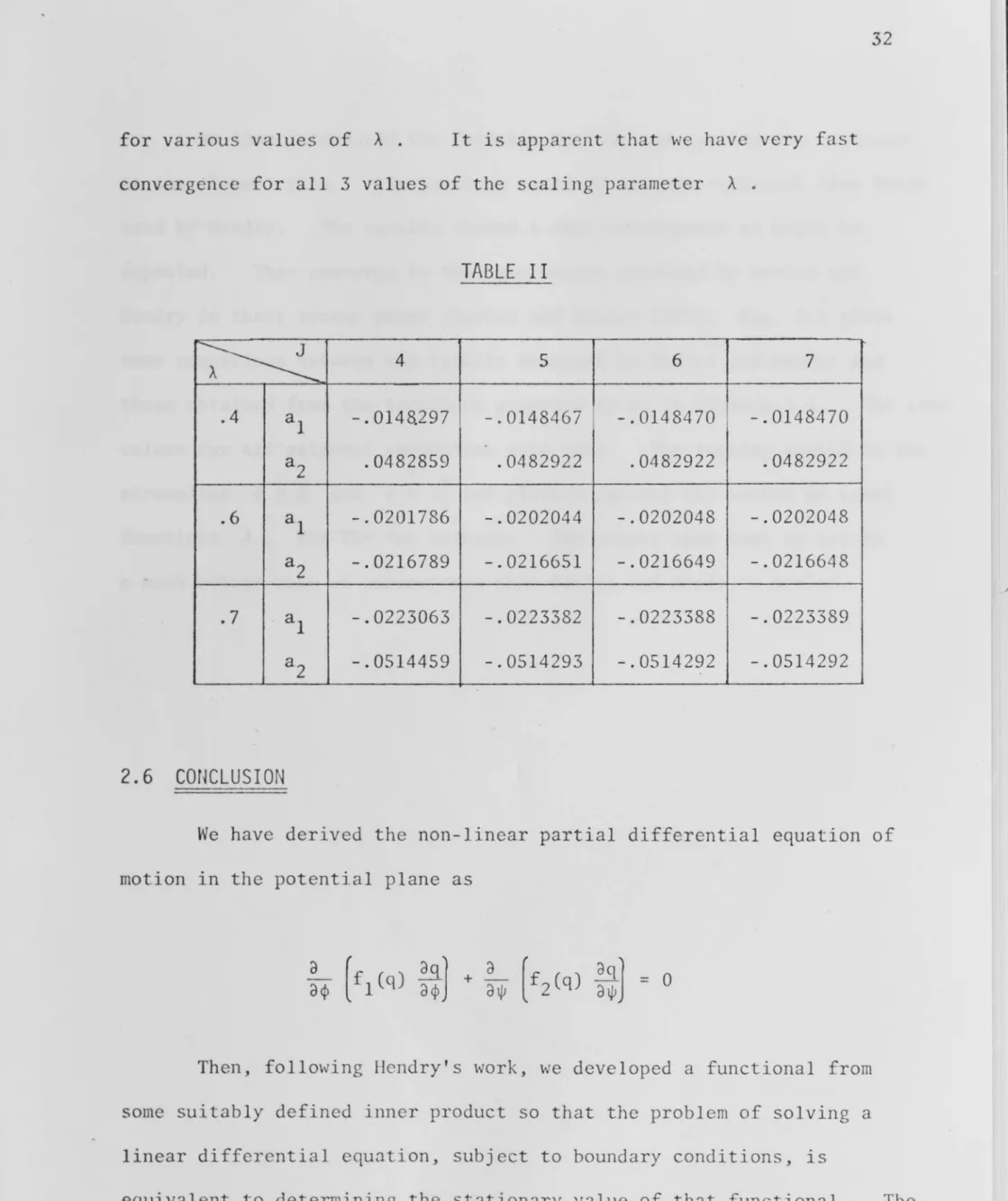
for varlOUS values of A . It is apparent that we have very fast

convergence for all 3 values of the scaling parameter A.

TABLE

~

.4 a

l -.0148.297 -.0148467 -.0148470 -.0148470 a

2 .0482859 .0482922 .0482922 .0482922

. 6 a

1 -.0201786 -.0202044 -.0202048 -.0202048 a

2 -.0216789 -.0216651 -.0216649 -.0216648

. 7 a

1 -.0223063 -.0223382 -.0223388 -.0223389 a

2 -.0514459 -.0514293 -.0514292 -.0514292

2.6 Cor~CLUS I ON

We have derived the non-linear partial differential equation of motion ln the potential plane as

Then, following Hendry's work, we developed a functional from some suitably defined inner product so that the problem of solving a linear differential equation, subject to boundary conditions, is

equivalent to determining the stationary value of that functional. The

Iterative Variational Method, using the trial functions not satisfying the

boundary conditions, was extended to the non-linear system above with the

We then introduced the Galerkin Method, and applied the technique to the channel flow. _{The matrices involved are now different from those} used by Hendry. _{The results showed a fast convergence as might be}

expected. _{They converge to the same values obtained by Davies and}

Hendry in their recent paper (Davies and Hendry 1975). Fig. 2.6 gives some comparison between the results obtained by Davies and Hendry and

those obtained from the technique proposed by us ln s~ction 2.4. _{The same} values for all relevant parameters were used. _{The turning angles on the} streamline tIJ

=

=

1.86

1.85

1.84

1.8386

4

Figure 2.1

:\=.6

5 ₆

Turning angle ~e against number of trial

function~ J for various streamlin s.

3

M

---~---.---~---;;---·--1}·02%

--_._---.---M

---4 5 6

Figure 2.2

7 J 3 4 5

Local Mach number M and angle

e

of trial functions J for various streamlines.

6 7 J

tN

~=~~

1 I £)

~=¥~

1

r

~=~~ I

~=O 1

--~~---'----~

,=n I

--<1>=0 <1>=-3.185 _<1>=-2.519

<1>=-1.727

Figure 2.3 _{Shape of the channel in the (x,y)-plane}

- - - - <1> constant

--- ~ constant

J=7

-

.--

-.-I

VJ

Error in 68

.04

.03

.02

.01

J=4

o

.4

Figure 2.4

.5 _{.6 . 7 . 8}

Error in !J

.03

.02

.01

.0

4

Figure 2.5

5 6 7

Maximum rror ln tun1ing angle against number

of trial functions J for various values of A .

-1.83

-1.8386 -1.84

4 ₅

Figure 2.6

6 7 8 9 10 _{4 5 6 7}

Turning angle 68 against number of trial functions J

() t='I _{our result}

o EJ _{Hendry's result}

8 _{9 10 J}

CHAPTER III

CASCADES OF

AEROFOILS

3. 1 INTRODUCTION

In this chapter we proceed to the problem of flow through cascades

of aerofoils. The description of the problem, together with the

mathematical formulation, is given in section 3.2. Then in section 3.3,

we deduce the various conformal transformations to map the complicated

potential plane onto a relatively simple region. This effects a

substantial reduction in the analytic difficulties attached to the selection

of a suitable form for the trial function for the velocity distribution.

In this, we make use of the approach adopted by Woods (Woods 1961), who

gave a conformal transformation mapping the potential plane of incompressible

cascade flow onto a semi-infinite, rectangular strip (figure 3.6).

We then extend this work to the case of compressible cascade flow

ln section 3.4. The final modified reglon turns out to be a square, over

which the trial function is defined. In section 3.5, the principles of

the Galerkin Method, described in the previous chapter, are applied to

cascade flow in general. In section 3.6, some relationships amongst the

mapping planes are investigated and some of the limiting values of terms

which are of relevance are worked out. This information is of considerable

use to us ln our later work. Lastly, in section 3.7, the general forms of

the residuals r. , and the matrix elements, relevant ln the proposed

1

non-linear iterations, are given in detail for the tria 1 function q of

3.2

DESCRIPTION OF THE PROBLEM

By a cascade of aerofoils, we mean an infinite set of similar

aerofoils at the same incidence, spaced at equal distance from each other

along the y-axis as shown In figure ~.l

A ' - - - - - H

y

... _,

---~~~~~77~~---~X

z

=

Figure 3.1

"

--

The solution to this problem is valuable because it is a first

approximation to the flow through the blading of an axial compressor,

especially at the high pressure end, where the blade height is small

(.,~'O{'

space between two blades to the IQIIgtk of the blade tend to infinity, the limiting case becomes the problem of a single aerofoil.

As ShO\ffi 1n figure 3.1, the aerofoils are equally spaced along the y-axis by a distance H. The flow is shown to have the upstream or inlet speed of q

u ' with the inlet angle of 8 u The dO\\TJlstream

or outlet speed at infinity is qd' with the outlet angle of 8 d . The repeat condition 1S the requirement that the flow at points

(x,y+nH) where n

=

separate from each aerofoil at some point on its upper surface, resulting in a wake of slowly moving turbulent fluid extending to infinity.

Different ways of treating this phenomena are discussed briefly in

Woods (Woods 1961 p. 19 ff). Our model, however, ignores the trailing edge (as has been mentioned), and the aerofoils, therefore, only close at infinity, conveniently bypassing the displacement property created by the wakes.

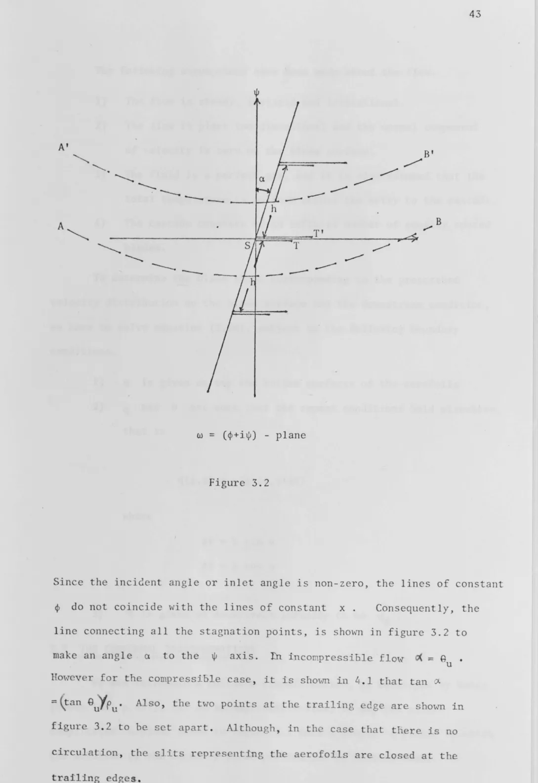
Now consider the representation of the flow in the potential plane as shmffi in figure 3.2. Note that, Slnce the surfaces of the

A'

~

"-.

'-...

.---

~

--

---

---

---T'

T

.---

--

----

_---

---

w

=

Figure 3.2

B'

/

B

~

Since the inciGcnt angle or inlet angle is non-zero, the lines of constant

~ do not coincide with the lines of constant x. _{Consequently, the}

line connecting all the stagnation points, is sho\ffi in figure 3.2 to make an angl e CL to the ~ aX1S. In incompre.ssiole f10\-[ _{= Q •}

u

Hmvever for the compressible case, it is sho~m in 4.1 that tan (J..

= tan

tJuYPu'

figure 3.2 to be set apart. Although, in the case that there is no

circulation, the sli ts repr s nting the aerofoils are closed at the

The following assumptions have been made about the flow.

1) The flow 1S steady, invjscid and irrotational.

2) The flow 1S plane two-dimensional and the normal component

of velocity 1S zero on the blade surface.

3) The fluid is a perfect gas, and it is also assumed that the

total temperature is uniform across the entry to the cascade.

4) The cascade consists of an infinite number of equally spaced

blades.

To determine the blade shape corresponding to the prescribed

velocity distribution on the blade surface and the downstream condition,

we have to solve equation (2.10), subject to the following boundary

conditions.

1) q is glven on top and bottom surfaces of the aerofoils

2) q and

e

that is

where

b¢>

=

b'¥

=

3) q 1S glven at downstream infinity to be qd'

3.3 THE CONFORMAL TRANSFOR

MATION

S

We now introduce a suitable transformation, as developed by Woods

(Woods 1961 p.487), for an incompr~ssible flow, to map the rather

complicated w-I lane shown in figure 3.2 onto a simple ~-pla~e, 1n which

First, we take the particular case of the incompressible flow

through the cascade for which both the downstream and upstream angles

are zero, as is shown in figure 3.3. _{The flow 1n the potential plane}

is shown in figure 3.4. _{We note that there is no circulation Slnce}

the inlet and outlet angles are zero, and therefore the slits representing

the aerofoils are closed (see section 4.1 for more detail). _{h 1S now}

the perpendicular distance from one aerofoil to another, and hence equal

to b~ (the jump 1n ~ from one blade to the next).

e

z - plane

'Figure 3.3

We will distinguish the potential plane of this flow from the one

shown in figure 3.4. _{If the length of the slits IS k, it can be} verified that the transformation

t = 1 - exp(-2nw

O/h) (3.1)

maps the slits into a single slit of length

t~

=

ln the t-plane shown in figure 3.5, taking the orIgIn of the wO-plane to be at the leading edge

F

S of one of these slits.

o

tPO

T'

h S ,,""====~O __ ... ______ .. __ .. ____ ~ <PO

0'" - - - - ... ... ..

-F'

TO

wo - plane Figure 3.4

F

F'

The t-planc IS In turn mapped into the ~-plane by the

transformation

1

t

= 2

which, In using .(3.1) gIves

1 - exp(-2nw

_o

_{= 2}

which may be written as

where

Wo

=

~

-

s}

2 2n

*

kn

r

=

_h

If we define n by,

*

cosh

n =

(3.2)

then _{the transformation (3.2) takes the point 4>}

_{o -}

onto the point 1.1

=

=

0

,

lJJ >

0 0 and 4>0

=

,

=

*

*

and (-n, n ) respectively. _{Furthermore, the opposite sides of the}

trailing edge streamline in the t-plane, tl

=

where t

=

=

*

. *

-n+ln

-n

E'

_o

T

-n+S

S

2

-s

S

So

1 0

- plane

Figure 3.6

n

*

n+in

y

The stagnation points So will coincide, ln this case, with the orlgln

of the z;;-plane. _{The streamlines t = 1 - exp(-2nW}

0/h) are mapped to

*

the lines y

=

=

and 0 < y < n are the opposite sides of the blades.

Now, if we consider the flow in figure 3.2 to be an incompressible

flow, then both wand

Wo

sense used ln Woods, w will consequently be an analytic function of w

o

'

and therefore of z;;.

~n

[q

dZ]

~

(3.3) T

=

q

and

~nrq ~

J

O (3.4)

TO

=

=

then, again In the sense used In Woods, both T and TO are analytic

functions of

s

-

.

By the repeat condition of the flow, we deduce that T and

are periodic, that is,

and

slnce the points ('IT,ll) and (-'IT,ll) would either be the same point

In the z-plane, or the corresponding points separated by the distance

nH, where n

=

The above information enables us to make use of the theory developed

In Woods (Woods 1961 §4.3), where the calculus of residues is employed to

write

(3.5)

and _(3.6)

Here _{8S and 80S} are the directions on the surface of the boundaries.

It is easy to see that _{8S and 80S will} differ only because of the