Received: 18 January 2017 Revised: 25 April 2017 Accepted: 02 May 2017
Accepted Manuscript Online: 03 May 2017
Version of Record published: 28 June 2017
Research Article
Reliability of an automatic classifier for brain
enlarged perivascular spaces burden and
comparison with human performance
V´ıctor Gonz ´alez-Castro
1, Mar´ıa del C. Vald ´es Hern ´andez
1, Francesca M. Chappell
1, Paul A. Armitage
2, Stephen
Makin
1and Joanna M. Wardlaw
11Department of Neuroimaging Sciences, Centre for Clinical Brain Sciences, University of Edinburgh, 49 Little France Crescent, Edinburgh EH16 4SB, U.K.;2Department of Infection, Immunity and Cardiovascular Disease, University of Sheffield, Royal Hallamshire Hospital, Sheffield S10 2JF, United Kingdom
Correspondence:V´ıctor Gonz ´alez-Castro ([email protected]) or Mar´ıa del C. Vald ´es Hern ´andez ([email protected])
In the brain, enlarged perivascular spaces (PVS) relate to cerebral small vessel disease (SVD), poor cognition, inflammation and hypertension. We propose a fully automatic scheme that uses a support vector machine (SVM) to classify the burden of PVS in the basal ganglia (BG) region as low or high. We assess the performance of three different types of de-scriptors extracted from the BG region in T2-weighted MRI images: (i) statistics obtained from Wavelet transform’s coefficients, (ii) local binary patterns and (iii) bag of visual words (BoW) based descriptors characterizing local keypoints obtained from a dense grid with the scale-invariant feature transform (SIFT) characteristics. When the latter were used, the SVM classifier achieved the best accuracy (81.16%). The output from the classifier using the BoW descriptors was compared with visual ratings done by an experienced neuroradiologist (Ob-server 1) and by a trained image analyst (Ob(Ob-server 2). The agreement and cross-correlation between the classifier and Observer 2 (κ=0.67 (0.58–0.76)) were slightly higher than be-tween the classifier and Observer 1 (κ=0.62 (0.53–0.72)) and comparable between both the observers (κ =0.68 (0.61–0.75)). Finally, three logistic regression models using clini-cal variables as independent variable and each of the PVS ratings as dependent variable were built to assess how clinically meaningful were the predictions of the classifier. The goodness-of-fit of the model for the classifier was good (area under the curve (AUC) values: 0.93 (model 1), 0.90 (model 2) and 0.92 (model 3)) and slightly better (i.e. AUC values: 0.02 units higher) than that of the model for Observer 2. These results suggest that, although it can be improved, an automatic classifier to assess PVS burden from brain MRI can provide clinically meaningful results close to those from a trained observer.
Introduction
Perivascular spaces (PVS), also known asVirchow–Robin spaces, are fluid-containing spaces that sur-roundthe walls of smallvessels andcapillaries in the brain as they go through the grey or white matter. PVS are microscopic, filledwith interstitialfluidandact asdrainage pathways for fluidandmetabolic wastes from the brain and, when enlarged, are visible in structural MRIsequences [1].High number of enlargedPVS has been reportedto be associatedwith worse cognition [2], active inflammation in multiple sclerosis plaques [3]or aging [4],depression at older ages [5], Parkinson’sdisease [6]andcerebralsmall vessel disease (SVD) [7].
[12]and[13] presentedcomputationalmethods to obtain quantificative measurements of PVS andvalidatedthe usefulness of their procedures in clinicalresearch, but both approaches are semi-automatic being, therefore, prone to interobserver variations andcouldbe time-consuming. [14]also proposeda methodfor quantifying PVS using high-resolution7TMRIscanners but the use of such fieldstrengths, although providing goodspatialresolution and signal-to-noise ratio, haslimitedclinicaluse. [15]use a Frangi filter whose parameters are optimizedby means of the ordered logit modelto enhance thedifferentiation between PVS andthe background, but is unsuitable for images with anisotropic voxels commonly usedin clinicalsettings (e.g. voxelsizes of0.5×0.5×6 mm) andstillrequires the (visual) rating of the PVS.
As an alternative to quantificative measurements, severalvisualrating scales that provide a qualitative assessment of the burden of PVS have been proposedin recent years. Potter et al. [16]reviewedthe ambiguities of these scales andcombinedtheir strengths todevelop the one that provedto be robust.However, as with any visualrecognition process, it is subject to observer bias.Making the PVS rating automatic (e.g. replicating the visualrating scale using image processing andpattern recognition) couldpotentially overcome these andalso thedrawbacks that the current methods of PVS segmentation have.
Computer vision andpattern recognition have already been successfully appliedto computer-aided diagnosis using MRI[17,18]andfor segmentation of brain structures orlesions [19-21].It has also been usedto assess markers of SVD qualitatively. For example,Chen et al. [22]proposeda framework basedon multiple instancelearning todistinguish between absent/mildcomparedwith moderate/severe SVDin computedtomography (CT) scans.
However, to the best of our knowledge, only two papers have addressedthe task of assessing automatically the PVS rating in brainMRIusing computer vision andpattern recognition techniques [23,24]. They exploredthe use ofdifferentdescriptors for this task, butdidnot analyse agreement with a human observer other than the one that providedthe groundtruth ratings or whether the predictors of the classification were clinically meaningful.Moreover, each of these two works evaluated differentdescriptors to characterize the brain region selectedfor classifying PVS burden andreport similarlevels of accuracy for the preferredschemes, albeit having validatedthe schemesdifferently (i.e. [23]uses cross-validation and[24] compares results on randomlydividedtrain andtest subsets). An overall evaluation of the schemes proposedso far for classifying the burden of PVS from brainMRIislacking.
In the present paper, we buildupon the work presentedin [23,24], comparing the performance of thedescriptors proposedby both studies for automatically classifying the burden of PVS using a support vector machine (SVM) [25]. We focus on the PVS in the BG, since moderate-to-severe PVS in this region (i.e. ratings 2–4) is a marker of cerebral SVD.We evaluate threedifferent types ofdescriptors:(i) statistics obtainedfromWavelet transform’s coefficients [26], (ii)localbinary patterns [27]and(iii) bag of visualwords (BoW) based descriptors, using keypoints obtainedfrom adense gridcharacterizedwith the scale-invariant feature transform (SIFT) characteristics.Moreover, we validate the results by comparing the predictions made by the automatic method(i.e. the classifier using thedescriptors that achieve the best performance) with the ratings from the two observers. Finally, we also investigate the applicability of this classifier to clinicalstudies, to assess if its outcome is clinically meaningful. The paper is organizedas follows: in‘Materials andmethods’section, thedataset andproposedmethods are explained.‘Results’section introduces the experimentalsetup andthe results of the experiments, which arediscussedin section titled ‘Discussion’. Finally, the conclusions andpossible futurelines of work are presentedin‘Conclusion andfuture work’section.
Materials and methods
Subjects and MRI protocol
We used data from 264patients who gave written informedconsents to participate in a study oflacunar stroke mech-anisms [28].
Figure 1.Anatomical regions and appearance of PVS.
Example of the anatomical regions where the PVS (arrowed) are rated: midbrain, BG and CS (from (A) to (C) respectively). Note the longitudinal appearance in the CS in axial view ((C) inset).
stroke or whose symptoms resolvedwithin 24h (i.e. transient ischaemic attack).It was approvedby the Lothian Ethics ofMedicalResearchCommittee (REC 09/81101/54) andthe NHS Lothian R&D Office (2009/W/NEU/14) andwas conductedaccording to the principles expressedin theDeclaration ofHelsinki.
BrainMRIwas conductedat baseline (i.e. there was a maximum of8 days between the stroke andthe scan) on a 1.5teslaGE Signa LXclinicalscanner (GeneralElectric,Milwaukee,WI), equippedwith a self-shielding gradient set andmanufacturer suppliedeight-channelphasedarray healcoil. For our analyses, we usedthe T2w images, acquired with TE147ms, TR 9002 ms, fieldof view 240×240mm, acquisition matrix 256×256, slice thickness: 5mm,1 mm interslice gap andvoxelsize0.469×0.469×6 mm. The reconstructedimage size (in voxels) is512×512×28. For tissue segmentation,diffusion-weightedandstructuralT1-weighted(T1w), T2w andgradient echo, acquiredas specifiedin [28]were also used.
PVS visual rating scale
The visualrating scale proposedby Potter et al. [16]was usedfor assessing the burden of PVS in the sample.It rates the PVS separately in three major anatomicalbrain regions, i.e. midbrain, BGandcentrum semiovale (CS) shown in Figure1–using T2wMRI. The rating isdone separately forleft andright hemispheres, but a combinedscore that represents the average of the PVS burden is given.
In each of these anatomicalregions, the rating can be0(no PVS),1(mild; 1–10PVS), 2 (moderate; 11–20PVS), 3 (frequent;21–40PVS) or4(severe;>40PVS)1.
Allvisualratings were made by two observers:a neuroradiologist (Observer1) with more than 25years of expe-rience who participatedin thedevelopment of the scale anda trainedimage analyst (Observer 2). The ratings were done blindto allclinicalinformation, each other’s results andany intermediate or finalcomputationalresults.
In the present paper, we focus only on the PVS in the BG, since moderate to severe PVS in this region (i.e. ratings 2–4) is a marker of cerebralSVD, which has been associatedwith cognitivedecline [10], vasculardementia andstroke [1]. An example of each of the ratings for the BGis shown in Figure 2.Wedichotomize the BGPVS scores into two
Figure 2.Basal ganglia PVS ratings using Potter et al. [16] scale.
Example for the PVS ratings in the BG, from 0 (none) to 4 (many) ((A–E) respectively) with black arrowheads pointing to some of the PVS.
classes as per [1], scores0–1(i.e. none or mildPVS burden) andscores 2–4(i.e. moderate to severe), to be our classes 0and 1respectively.
Image preprocessing
The guidelines for the visualrating of PVS according to this scale states that the rating shouldbedone on the slice with the highest number of PVS, so as to minimize inconsistencies andintra-/interobserver variationsdue to interslice variations in PVS visibility, varying number of PVS ondifferent slices and double counting oflinear PVS [16].In case of the BGregion, this slice shouldbe chosen among the slices with atleast one characteristic BGstructure, as indicated by [12]. A pipeline to extract the BGregion andfindthe axialslice (from the BG) with the highest number of PVS for each subject, wasdeveloped.
The first step of this pipeline is to automatically segment the intracranialvolume and CSF on the T1w images. This was achievedusing optiBET [29]andFMRIB softwarelibrary (FSL)-FAST [30]respectively. The secondstep is to, also automatically, extract allsubcorticalstructures, which was achievedusing other tools from the same FSL as is describedin [28]. Thereafter, from the slices that containedBGstructures, we selectedthose in which the totalarea of these structures was more than5%of the intracranialareadefinedon the slice.
On each of the BGslices initially selected, a polygon enclosing the BG, internalandexternalcapsules andthalami was automaticallydrawn byjoining anatomicalpoints in the insular cortex, the closest points to them in thelateral ventricles (frontalandoccipitalhorns) andthe intercept of the genu of the corpus callosum with the septum;and subtracting from it the region occupiedby theCSF. These steps are illustratedin Figure 3.
Figure 3.Graphical representation of the steps for delineation of the basal ganglia region
Steps of the BG segmentation: (A) Detection of the vertices in the insular cortex (1), lateral ventricles (2) and genu (3); (B) creation of the polygon; (C) subtraction of the CSF from the BG polygonal region and (D) segmented BG region.
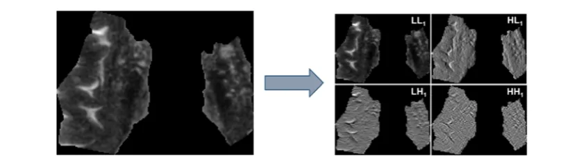
Figure 4.First-level DWT decomposition of the BG region from a T2w image.
Example showing the graphical representation of the values of the four matrices of coefficients (i.e. LL, LH, HL and HH) (right hand side) obtained after applying the discrete wavelet transform (DWT) to the region shown at the left hand side.
Descriptors
Descriptors based on the Wavelet transform
The information representedby spatialfrequencies has often been usedfor texturedescription with successfulresults [32].Due to its frequencydomainlocalization capability, we have appliedthediscreteWavelet transform (DWT) to each selectedregion to characterize their textures.We have usedtheHaar family of wavelets, which have already been successfully usedin other medicalimage classification applications [26]. TheDWT extracts thelow andhigh frequency components of a signal, so that they can be analysedseparately.
When the transform is appliedto an image, four matrices of coefficients are obtained:namely LLi, LHi,HLiand
HHiwhereistands for thelevelofdecomposition, which represent the approximations and details in the vertical,
horizontaland diagonal directions respectively. They can be seen in the example that Figure4illustrates.
[image:5.595.61.485.408.524.2]Figure 5.Example of the names of the coefficient matrices after a three-level DWT decomposition.
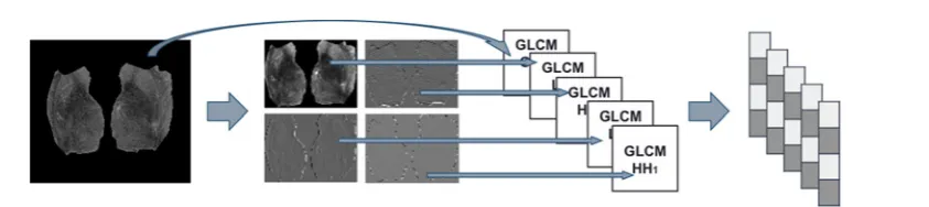
Figure 6.Diagram showing how the wavelet co-occurrence feature (WCF) descriptors are built.
One of thedescriptors we usedis basedon theDWT, andit is built using the mean andS.D. of the histograms of the originalimage andeach one of the matrices of coefficients yieldedafter threeDWTlevels (i.e. LL1, LH1,HL1,
HH1, LL2, LH2,HL2,HH2, LL3, LH3,HL3and HH3).Hence, we represent each region by a vector of 26 features. This
descriptor is known asWavelet statisticalfeatures (WSF) [26,32].
The otherdescriptor basedon theDWT is built using the features proposedby [33] derivedfrom the greylevel co-occurrence matrix (GLCM) of the originalimage andeach of the the coefficient matrices obtainedafter the first DWTlevel(i.e. LL1, LH1,HL1and HH1). The features extractedfrom eachGLCMare concatenatedto form the final
descriptor. Adiagramdepicting this process is shown in Figure 6.
To achieve some invariance to rotation, we averagedthe features extractedfromGLCMs computedwith orienta-tions0,45, 90and 135◦. Thesedescriptors are called WCF [26,32].In this work, we assessedtwo variants of theWCF descriptors,WCF4and WCF13,depending on whether we extracted 4or13 features from theGLCMs respectively.
WCF4is built using theHaralick featuresContrast,Correlation,EnergyandHomogeneity, and WCF13is formed
using allfeatures proposedby [33]except theMaximal Correlation Coefficient. These twodescriptors showedgood performance in [34].
Local binary patterns
Localbinary patterns (LBP) were introducedby [27].In the original, version they workedwith a 3×3 pixelblock, but LBPs werelater generalized, so size of the neighbourhoodandnumber of sampling points were parameters of the method.Given a pixelcwith co-ordinates (xc,yc), a pattern code is calculatedby comparing it with the value of itsP
neighbours separatedby adistanceR, which in our case is1, as per (eqn1).
LB PR,P =
P−1
p=0
s gp − gc
2p (1)
wheregcandgpare the grey-levelvalues of pixelcanditsp-th neighbour, andfunctions(gp–gc) isdefinedas:
s gp − gc
=
⎧ ⎨ ⎩
1ifgp − gc 0
0ifgp − gc <0
Finally, the whole image isdescribedby means of a histogram of the LBP values of allpixels, given by (eqn1). As the position of thefirstneighbour (i.e.p=0) is fixed, it being the pixelon the right handside ofc, the LBPR,Poperator is
not invariant to rotation.We remove such effect of rotation using the rotation invariantlocalbinary pattern,LB Pri R,P,
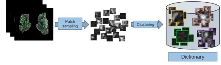
[image:6.595.125.547.198.292.2]Figure 7.How the dictionary is created.
Small square patches are extracted from each basal ganglia region, which are characterised by means of the descriptors and grouped to form the ”dictionary”.
As certainlocalbinary patterns represent fundamentalproperties of texture, providing the vast majority of patterns present in textures [27], while others are known to belessdescriptive of the texture,Ojala et al. [27]introduceda measure of’uniformity’U(LBPR,P), which counts the number of spatialtransitions (i.e. bitwise0/1changes) in a
binary pattern LBPR,P for LBPR,Pless than 2 (i.e. LBPriuR,P2) as expressedin (eqn 2).
LB PRriu,P2=
⎧ ⎨ ⎩
P−1
p=0s(gp−gc) ifU(LB PR,P)2
P+1 otherwise ,
(2)
As the BGregions andthe PVS are not very big, we triedto keep the texture analysis aslocalas possible, so in this work, we have usedthe valuesR=1andP=8. The final descriptors we use are the histograms of the accumulated output of LBP1,8, LBPri1,8andLBPriu1,82operating in each BGregion.
BoW
The BoWmodel[35]represents each image as a function of the frequency of appearance of certain visualelements, calledvisualwords. The set of visualwords is calledthedictionaryorcodebook.
To buildthedictionary, a set of keypoints from each image are sampled. Aroundeach keypoint, a smallsquare region (i.e. patch) is extractedandcharacterizedby means ofdescriptors that retrieve information about the distri-bution of its pixels intensities. After that, thedescriptors of the patches are clusteredintoKgroups, each one having a prototype feature vector which is calledvisual word. This process isdepictedin Figure7.
In this work, we use adense gridfor sampling the keypoints andthek-means clustering method[36]for forming the visualwords. The process of creating thedictionary is performedin each iteration of the cross-validation using the subsets of images usedfor training.We assessed different numbers of visualwords to evaluate their impact on the classification.
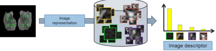
Once thedictionary is built, each image of thedataset isdescribedby means of a process calledimage
represen-tation. This consists of repeating, for each image, the same process of keypoint selection andcharacterization used
in the creation of thedictionary, using also the same methods. Then, for each‘new’patch, we findthe visualwordof thedictionary that is most similar to it by means of calculating the Euclideandistance between theirdescriptors.
The histogram of the visualwords representative of allpatches in an image is usedas its final descriptor. The image representation process is illustratedin Figure8.
In this work, the patches aredescribedusing the SIFT [35]. Basically, SIFTdescriptors are basedon histograms of orientedgradients computedfrom the intensities of the regions that result fromdividing a16×16 pixelsquaredpatch aroundeach keypoint into16 subregions of4×4pixels each.Moredetails about SIFT can be foundin [35].Despite these consisting of twodifferent parts, keypointdetector andpatchdescriptor, we only use the patchdescriptor as we are sampling the keypoints in adense grid.
Classification
Figure 8.How the image representation is carried out.
Once the ”dictionary” is formed, the histogram of the visual words representative of all patches is used as the final descriptor.
(i.e. margins) to the instances of the positive andnegative classes in the trainingdataset.One of the parameters of SVMis the cost parameterC, which controls the trade-off between classes allowing training errors andforcing rigid margins.
SVMis alinear classifier:it tries to separate thedata using alinear hyperplane. There are cases where thedata are notlinearly separable.In those cases, SVMmay use thekernel trick:a kernelfunction K (x,x) may transform the data into a higherdimensionalspace where it is possible to separate itlinearly. After evaluatingdifferent kernels (i.e. linear, radialbasis function, sigmoid), the best results were achievedwith the radialbasis function (RBF) kernel:
Kx’,x = exp −γx’−x2
(3)
We refer the reader interestedin moredetails about SVMto [40].
We use severalcombinations of the regularization parameterC(i.e.1,5,10,50,100, 250and 500) andγ(i.e.10–5,
10–4,10–3,0.01and 1), assessedwith all descriptors, to findthe optimalconfiguration.We use the implementation providedin thelibSVM library2[41].
Validation of the classifier
We validatedthe classification with a stratifiedfive-foldcross-validation as follows. The whole set, representedby the descriptors explainedin‘Descriptors basedon theWavelet transform’,‘Localbinary patterns’and ‘BoW’sections, was randomly partitionedinto five equal-sizedsubsets with the samedistribution as the originalset.Of the five subsets, four were usedto train the classifier andthe remaining one was usedas the test set. This process was repeatedfive times using adifferent subset each time as test set. The five results from the five folds were averagedto provide the finalresults.
This cross-validation process was repeatedten times, andthe ten results were averagedto avoidpossible biasdue to a random separation of the folds.Data were normalizedso that they hadmean0andS.D.1.
The overallresults were validatedin terms of accuracy, sensitivity andspecificity, using thedichotomizedratings ofObserver1as groundtruth.
Statistical analyses
Thedescriptors that achievedthe best performance wouldbe usedin a realautomatic visualrating application. There-fore, we analysedthe agreement of the visualratings between the automatic classifier basedon thosedescriptors and between each observer.We also analysedthe association between the outcome of each PVS rating (i.e. from each ob-server andfrom the automatic classifier) andclinicalparameters known to be relatedto PVS burden in the patients that comprise this sample (see‘Subjects and MRIprotocol’section).
Interobserver agreement
Wedeterminedthe weightedκcoefficient of the PVS ratings in the BGregion (scale0–4) between observers as per
http://vassarstats.net/kappa.html(Copyright RichardLowry 2001–2015).We also performedmarginalhomogeneity tests of the BGPVS visualratings (scale0–4) using the software application mh.exe ver.1.2 (2016-03-01) (byJohn Uebersax).
Afterdichotomizing the BGPVS visualratings producedby both the observers, wedeterminedtheκcoefficient be-tween the observers andbetween the automatic classifier andeach observer, using theκfunction inMATLAB R2015a
Table 1Distribution of the visual ratings in the sample
PVS rating 0 1 2 3 4 Total
Number of images (%) 5 (1.89%) 128 (48.48%) 68 (25.76%) 44 (16.67%) 19 (7.20%) 264
(Copyright c2007,GiuseppeCardillo, updated23Dec 2009,http://uk.mathworks.com/matlabcentral/fileexchange/ 15365-cohen-s-kappa/content/kappa.m).We also conductedtheMcNemar’s test between the ratings producedby the expert (i.e.Observer1) andthe automatic classifier to investigate whether the marginalfrequencies between both were or not equal.
Clinical validation
The following clinicaland demographic parameters were available for each study participant:age, hypertensive (or not) classification, stroke subtype (lacunar or cortical) classification andscores ofWMH, atrophy andSVDburden. WMHwere codedusing Fazekas scores, for periventricular (PV) and deeplesions separately in theleft andright hemispheres anda combinedscore for both hemispheres was recorded[42]. Brain atrophy was codedusing a validated age-relevant template [43], with superficialand deep atrophy codedseparately ranging from none to severe on a scale of1–6 according to the centiles into which the template isdivided, being1(<25th), 2 (25–50th), 3 (50–75th), 4(75–95th),5(>95th) andif>>5, 6 is used. Totalatrophy was calculatedas the average ofdeep andsuperficial atrophy scores. SVDwas codedas per [44](0–4), which confers a point for each of the following conditions:if1or more cavitated, old lacunarlesions are present, if Fazekas PVscore3 and/or FazekasDeep score2, if BGPVS score is2 as per Potter et al. [16](i.e. moderate-to-extensive), andif more than1, brain microbleedis present.
We calculated the non-parametric bootstrapped correlations between BG PVS scores (before and after di-chotomization, from observers andfrom the automatic classifier) andeach clinicalvariable.We also performed bi-nomialmultivariablelogistic regression to evaluate the clinicalusefulness of our machine-learning scheme as per [16]andits sensitivity in various models. Thelatter was evaluatedby comparison of correlatedreceiver operating characteristic (ROC) curves obtainedfrom three models that have outcome variable as thedichotomizedPVS rating from (A) the automatic classifier, (B)Observer1and(C)Observer 2. The first model(i.e. model 1) hadthe following predictors:age, totalatrophy, hypertension, Fazekas score, whether the patient hada previouslacunar infarct or not, index stroke subtype andSVDscore. The secondmodel(i.e. model2, implementedin [16]) hadthe same predictors as model 1with the exception of SVDscore. The thirdmodel(i.e. model3) also hadthe predictors of model 1with the exception of Fazekas score andwhether the patient hada previouslacunar infarct or not, as these two parameters are contemplatedwithin the SVDscore. These analyses weredone usingMATLAB R2015a.Of note, the PVS outcome variable is also a contributor to the SVDscore.
Analysis of the robustness against imaging confounds
Allscans of the primary study that provided data for this analysis underwent quality checks. None of the T2-weighted sequences were corruptedby visible movement artefacts that couldaffect the automatic PVS rating procedure pre-sented.However, there are other confounds that couldhave influencedthe results.We calculatedthe number of scans misclassifiedon each of the ten iterations that contributedto the finalresult, on the absence andpresence of the fol-lowing imaging confounds visually identifiedbyObserver 2 in the BGregion blindto the neuroradiologicalreports: WMHfoundeither bilaterally andscatteredthroughout the region or as a single cluster possibly indicative of a recent or oldsubcorticalinfarct,lacunes (symptomatic or asymptomatic), recent or oldcorticalstrokes that partially affect the region, globus pallidus partially or totally hyperintense, partialvolume effects of theCSF, anda combination of two or more of these factors.
We also countedthe number of scans misclassifiedon each iteration for those people who hadalacunar infarct neuroradiologicallydetermined, regardless of whether it was visible on T2-weightedin the BGregion or not. This analysis wouldallow us todiscuss whether the occurence of a recentlacunar infarct influencedthedescriptors used by the classifier.
Results
LBP1,8 50 10 68.34 70.49 66.21 2.54 2.18 3.51 LBPri
1,8 50 10–4 70.02 75.95 64.01 1.02 1.22 1.49
LBPriu21,8 10 0.01 74.22 81.97 66.37 0.70 1.39 1.57
WCF4+ LBPri
1,8 250 10–4 78.84 79.84 77.80 1.12 1.60 1.25
WCF13 + LBPri1,8
100 10–4 78.13 78.62 77.58 1.16 2.07 1.55
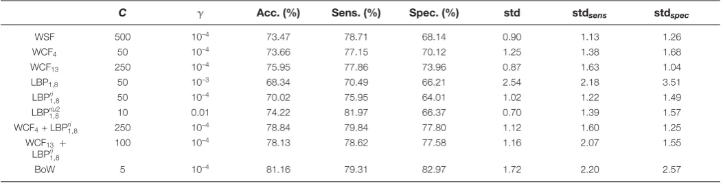
BoW 5 10–4 81.16 79.31 82.97 1.72 2.20 2.57
[image:10.595.27.554.96.230.2]The cost parameter for the SVM scheme (C) and the regularisation parameter of the radial basis function kernel (γ) for which the best results with each set of descriptors (i.e. first column on the left) were obtained, are provided. Abbreviations: acc., average accuracy; sens., sensitivity; spec., specificity.
Table 3κcoefficient, S.E.M. and 95% CI, given the observed marginal frequencies between each observer and the automatic classification method
κ S.E.M. 95% CI
Obs. 1 compared with classifier 0.6228 0.0481 (0.5286–0.7170)
Obs. 2 compared with classifier 0.6743 0.0455 (0.5851–0.7635)
Results of the SVM classification
Table 2 shows the best results using thedescriptors basedon theWavelet transform (i.e.WSF,WCF4and WCF13), the
descriptors basedonlocalbinary patterns withR=1andP=8(i.e. LBP1,8, LBPri1,8andLBPriu1,82), the fusions of the
descriptorsWCF4and WCF13with LBPriu1,82andthedescriptors basedon the BoWmodel.
The bestdescriptor in terms of overallaccuracy was thedescriptor basedon the BoWmodel(81.15%) using a dictionary with175visualwords, followedby the fusion ofWCF4andLBPriu1,82(78.84%).Moreover, the former reached
a sensitivityjust slightly worse than thelatter. The highest sensitivity is achievedby LBPriu2
1,8, but its specificity is much
worse than the BoW-based descriptor.It is also remarkable that, whereasWCF4does not get a goodaccuracy on its
own, its accuracy improves by7%when it is fusedwith the LBPriu2
1,8 descriptor.
The automatic classifier usedin the following sections willbe the SVMbasedon thedescriptors that achievedthe best overallaccuracy (i.e. thedense-SIFT basedBoWmodel, with the SVMparametersC=5andγ=10–4using the
dictionary of175visualwords).Once the visual dictionary is createdandthe classifier is trained, this methodtakes 0.0477s todescribe andclassify each image.
Interobserver variability
The agreement of the BGPVS ratings (scale0–4) betweenObservers1and2 wasκ=0.8269, S.E.M.: 0.0398, 95% CI:(0.749–0.9048). The maximum possiblelinear-weightedκ, given the observedmarginalfrequencies was0.8729. McNemar’s tests for each rating (0–4), and McNemar’s tests of equalthresholds were significant in rating1(P<0.003). The agreement of thedichotomizedBGPVS ratings betweenObservers1and2 wasκ=0.6822, S.E.M.: 0.0369 and 95% CI:(0.6099–0.7545). The maximum possiblelinear-weightedκ, given the observedmarginalfrequencies was 0.8486.
[image:10.595.37.555.306.353.2]Table 4Two-by-two table between the ratings done by the expert (i.e. Observer 1), the predictions of the classifier and ratings from Observer 2
Ratings Auto. Classifier Observer 2
0 1 0 1
Observer 1, rating 0 104 29 102 31
[image:11.595.41.567.184.260.2]Observer 1, rating 1 18 113 11 120
Table 5Non-parametric bootstrapped cross-correlation matrix for PVS ratings in the BG region
Parameter Observer 1 scale 0–4
Observer 1
dichotomized Observer 2 scale 0–4
Observer 2
dichotomized Automatic classifier
Observer 1 (0–4) 1 0.9317 0.8130 0.6828 0.6588
Observer 1 (0–1) 1 0.7341 0.6901 0.6464
Observer 2 (0–4) 1 0.9057 0.7127
Observer 2 (0–1) 1 0.7030
[image:11.595.42.563.313.413.2]All correlations shown were significant withP<0.0001.
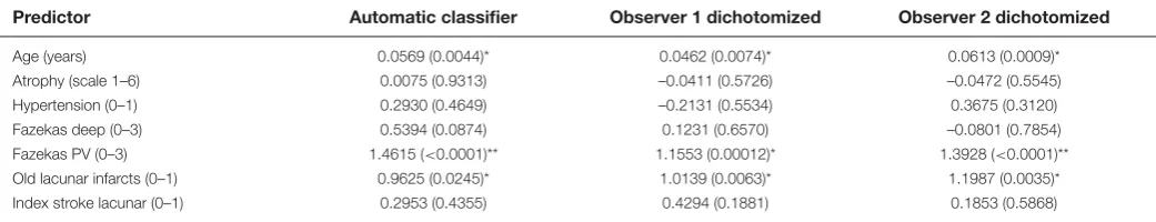
Table 6Coefficient estimates and significance (B (P-value)) of the associations for each predictor (i.e. clinical parameter) for model 2
Predictor Automatic classifier Observer 1 dichotomized Observer 2 dichotomized
Age (years) 0.0569 (0.0044)* 0.0462 (0.0074)* 0.0613 (0.0009)*
Atrophy (scale 1–6) 0.0075 (0.9313) –0.0411 (0.5726) –0.0472 (0.5545)
Hypertension (0–1) 0.2930 (0.4649) –0.2131 (0.5534) 0.3675 (0.3120)
Fazekas deep (0–3) 0.5394 (0.0874) 0.1231 (0.6570) –0.0801 (0.7854)
Fazekas PV (0–3) 1.4615 (<0.0001)** 1.1553 (0.00012)* 1.3928 (<0.0001)** Old lacunar infarcts (0–1) 0.9625 (0.0245)* 1.0139 (0.0063)* 1.1987 (0.0035)*
Index stroke lacunar (0–1) 0.2953 (0.4355) 0.4294 (0.1881) 0.1853 (0.5868)
The outcome variable is the dichotomized PVS score. *P<0.05, **P<0.001
Clinical validation
Bootstrapped correlations between the PVS ratings and with the clinical parameters
Visualratingsdone byObserver1(dichotomizedandnotdichotomized),Observer 2 (dichotomizedandnot di-chotomized) andthe automatic classifier were equally, significantly andpositively correlatedwith age, PVS ratings in CS (dichotomizedandnot), atrophy (deep andsuperficial), Fazekas (deep andPV), hypertension, old lacunar infarcts andSVDscore. None of the BGPVS ratings correlatedwith index stroke subtype (lacunar or cortical), andallwere highly andsignificantly correlatedwith each other as Table5shows.
Applicability in clinical research
Table 6 shows the results of the binomialmultivariablelogistic regression. Age, Fazekas PVscores andthe presence of old lacunar infarcts were significant andnegatively associatedwith allBGPVS scores (i.e. thosedone by both observers andby the automatic classifier), as in [16]. The coefficient estimates tabulated(B) express the effects of each predictor variable on thelog odds of being in one class (i.e.1or0) comparedwith the reference class (i.e.1or0 as perObserver1).
Sensitivity analysis
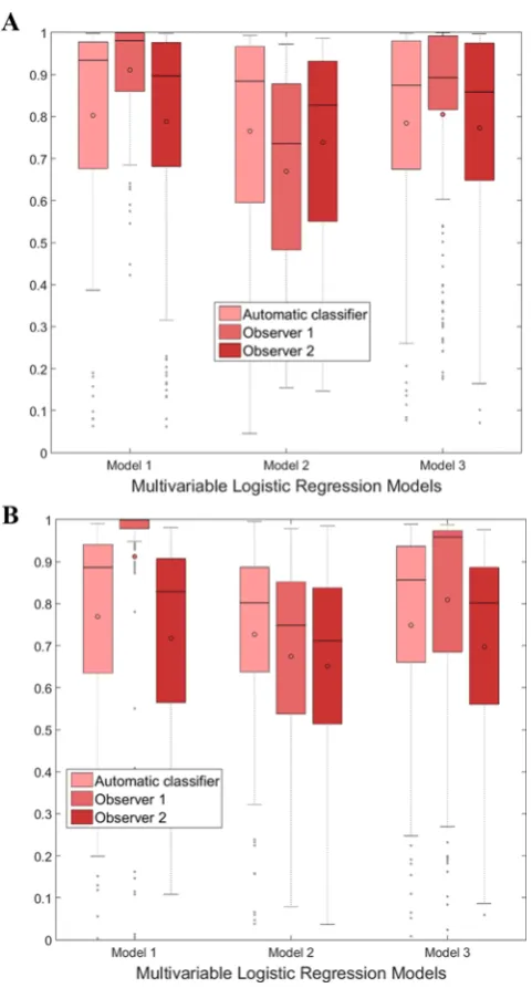
Figure 9 shows the predictedprobabilities of the outcome variables for each model. Thedistribution of the predicted ‘0’s and ‘1’s to be0and 1respectively for the classifier and Observer 2 were similar across allthe models. Alloutcomes (i.e. PVS ratings from the classifier,Observers1and2) were consistently poorer for model2, whichdoes not include SVDscores as predictor, than for the other two models. The PVS ratings fromObserver1were particularly sensi-tive to the presence andabsence of the SVDscores as predictor in the model, being exceptionally high when more components of the SVDscore (including it) were included(i.e. model 1).
Figure 9.Illustration of the results of the multivariable logistic regression models.
Boxplots showing the distributions of the predicted probabilities of the outcome variable ‘1’ (A) and ‘0’ (B) (i.e. PVS ratings from the automatic classifier, from Observer 1 or Observer 2) for each logistic regression model.
2) also for each model. The area under the curve (AUC) from the automatic classifier experiences theleast variation across the three curves: 0.93,0.90and 0.92 for models1, 2 and3 respectively (maximum variation 3%) indicating highest consistency in modelaccuracy, followedbyObserver 2 (maximum variation5%).
Performance on the presence/absence of imaging confounds
Figure 10.Receiver Operating Characteristics (ROC) for each classification.
ROC curves showing the performance for each outcome variable in the regression models 1, 2 and 3 ((A), (B) and (C) respectively). In model 1, (A) AUCs of the classifier, Observer 1 and Observer 2 were 0.9265, 0.9813 and 0.9074 respectively. In model 2, (B) AUCs of the classifier, Observer 1 and Observer 2 were 0.9041, 0.8395 and 0.8622 respectively. In model 3, (C) AUCs of the classifier, Observer 1 and Observer 2 were 0.9152, 0.9411 and 0.8934 respectively.
Table 7Number of scans misclassified per number of iterations, on the presence/absence of imaging confounds
Confounds Total number of scans Number of scans misclassified
1–3 iter. 4–6 iter. 7–10 iter.
Unilateral WMH 31 4 1 3
Lacunes (symptomatic or not) 25 4 4 3
Bilateral WMH 30 5 0 5
Cortical stroke/CSF partial vol. 7 0 0 2
Globus pallidus hyperintense 5 1 1 1
Two or more of the above 56 4 3 9
None 110 12 8 15
Lacunar stroke 119 17 5 15
Discussion
[image:13.595.46.567.517.642.2]lowing the visualrating guidelines for PVS from Potter et al. [16](http://www.sbirc.ed.ac.uk/documents/epvs-rating
-scale-user-guide.pdf), which are basedon assessing the PVS from a region of interest on the axial MRIslice with the most visible PVS. Allagreements between the automatic classifier, thedichotomizedratings of the experienced neu-roradiologist (Observer1) andthose from the trainedobserver (Observer 2), as shown in‘Interobserver variability’ section were above0.6.However, the agreement between thedichotomizedratings from both observers (κ=0.6822) was slightly higher than the agreement between the classifier andany of the observers (0.6228withObserver1and 0.6743 withObserver 2). The fact that the classifier hadbetter agreement withObserver 2 than withObserver1might be becauseObserver 2 followedthe same guidelines usedtodesign the pipeline for the automatic classifier, whereas Observer1may have also appliedtheir individualexperience andneuroradiologicalknowledge while rating the PVS. The cross-correlation between the classifier output andthedichotomizedratings of both observers, shown in Table5, followedthe same pattern:the correlation of the classifier withObserver 2 was higher than withObserver1(0.7030 and 0.6464respectively). This cross-correlation between the output of the classifier andthedichotomizedratings of Observer 2 (0.7030) was comparable andeven slightly higher than between thedichotomizedratings of both the observers (0.6901).
The statisticalmodelbuilt to evaluate the applicability of the automatic classifier to the clinicalresearch showed excellent andsimilar goodness-of-fit irrespective of whether the outcome variable was the automatic classifier (AUC
=0.90),Observer1(AUC=0.84) orObserver 2 (AUC=0.86). Also, age, the burden of PV WMH(i.e. Fazekas PV) andthe presence of old lacunar infarcts were associatedwith the PVS burden irrespective of whether these were rated automatically or visually by any of the observers, proving the usefulness of the automatic framework proposed. A separate sensitivity analysis of this andsimilar correlatedmodels showedthat the automatic classifier was theleast susceptible to be influencedby the overallburden of SVDshown in theMRIscan while the ratings from the neuro-radiologist capturedbetter the fullflavour of the SVDfeatures. Thedegree in which this result was favouredby the single-slice approach adoptedby the classifier [12,16]is not known. Further evaluation on the whole extent of the three anatomicalregionsdefinedby [16], with addedscrutiny to excludelacunes is needed. Nevertheless, given that the accuracy of the classifier on the presence of imaging confounds was notdifferent from it in the absence of them, andthat the output was quite robust against the whole SVDburden, wedo not foresee any problem for this automatic classification scheme to be appliedtolongitudinalor multicentre studies, aslong as the training andtestingdatasets have similar acquisition protocols.
A possiblelimitation of the present work is the fact that the segmentation of the BGregion is not always accurate (due to, for example, not finding the anatomicalpointsdescribedin‘Image preprocessing’section), causing a po-tentialmisclassification. As we wantedto assess the validity of a fully automatic method, we kept those suboptimal segmentations. Anotherlimitation of the study may be thedichotomization of the visualratings usedin the automatic classification.Due tolimitations in the sample size, we neededto simplify the classification, so wedichotomizedthe visualrating scale as it wasdone in recent studies [1]:a reliable five-class classification modelis not possible to be trainedwith such few instances in some classes (e.g. out of 264subjects there were only five with a rating0or19 with rating4). Further analyses using bigger samples andconsidering the fullratings (i.e.0–4) needto bedone.
Conclusion and future work
In the present paper, we have proposedan automatic framework basedon image analysis andmachinelearning to predict the burden of enlargedPVspaces on the BGas‘none or few’or‘moderate to severe’basedon the PVS visual rating scale [16].We compared differentdescriptors computedfrom the BGregion. The BoW-based descriptors achievedthe best accuracy (81.16%) in the classification, carriedout using a SVMtrainedusing the visualratings providedby an experiencedneuroradiologist (i.e.Observer1) as groundtruth.
The cross-correlation with theObserver 2 (0.7030) is also higher than that with theObserver1(0.6464), andslightly higher than that between both the observers (0.6901).
Finally, we built three correlated logistic regression models with some clinicalvariables as independent variables andthe ratings predictedby the automatic methodandboth observers as outcome variables and demonstratedthat although the automatic classifierdoes not capture the overallSVDseverity, it can be usedin clinicalresearch as it consistently gives a meaningfuloutput in relation to clinicalparameters.
For future work, we willtry to improve the classification performance by means of extracting the whole BGregion anduse the information from allslices where the extractedregion appears (i.e. 3Danalysis), as it may provide infor-mation that we are currently not taking into account.We willalso try to usedata from patients from other studies to increase our sample size andperform a five-class classification (i.e. ratings from0to4). Supervisedmachine-learning schemeslike the one presentedhere wouldrequire the groundtruth PVS counts or segmentations from alarge number ofdatasetsdone by an expert to be able to count and/or segment PVS. Suchdata are currently unavailable.However, the output from this classifier couldbe usedas input to the fully automatic PVS unsupervisedsegmentation approach developedby [15], (mentionedin the‘Introduction’section) which needs the PVS ratings to tune its algorithm and make it fully automatic. Finally, the classifier presentedhere couldbe adaptedto get the visualrating of the PVS in theCS.
Clinical perspectives
• In the brain, enlarged PVS are commonly assessed visually, for which several rating scales exist. However, for epidemiological and large clinical database analyses, there is a need for a fully automatic rating of the PVS load that overcomes interobserver and interscale differences, which the current study aims to address.
• The performance of the three different types of descriptors were assessed, with the SVM classifier achieving the best accuracy with the BoW-based descriptors. These outputs were compared with visual ratings made by an experienced neuroradiologist (Observer 1) and by a trained image analyst (Observer 2), with agreements and cross-correlations between the classifier and Observer 1, the classifier and Observer 2, and comparable between both observers beingκ=0.67,κ=0.62 and V=0.68 respectively. Models using clinical variables as independent variable showed that the goodness-of-fit of the model for the classifier was good and slightly better than that of Observer 2.
• An automatic classifier can be used to assess PVS burden from brain MRI, and can provide clin-ically meaningful results. The automatic scheme proposed can be used for large epidemiological studies and clinical databases, as it has been shown to be unbiased to the coexisting pathologies and is consistent.
Acknowledgements
We thank the study participants, radiographers and staff at the Brain Research Imaging Centre Edinburgh, SINAPSE (Scottish Imaging Network A Platform for Scientific Excellence) Collaboration Centre. We also thank the Wellcome Trust for providing the data.
Funding
This work was supported by the Wellcome Trust [grant number 088134/Z/09]; and the Row Fogo Charitable Trust [grant number BRO-D.FID3668413].
Author contribution
Functional MRI of the Brain; FSL, FMRIB software library; GLCM, grey level co-occurrence matrix; LBP, local binary pattern; PV, periventricular; PVS, perivascular space; ROC, receiver operating characteristic; SIFT, scale-invariant feature transform; std, standard deviation; SVD, small vessel disease; T1w, T1-weighted; T2w, T2-weighted; WCF, wavelet co-occurrence feature; WMH, white matter hyperintensity; WSF, Wavelet statistical feature.
References
1 Potter, G.M., Doubal, F.N., Jackson, C.A., Chappell, F.M., Sudlow, C.L., Dennis, M.S. et al. (2015) Enlarged perivascular spaces and cerebral small vessel disease.Int. J. Stroke10, 376–381
2 Maclullich, A.M.J., Wardlaw, J.M., Ferguson, K.J., Starr, J.M., Seckl, J.R. and Deary, I.J. (2004) Enlarged perivascular spaces are associated with cognitive function in healthy elderly men.J. Neurol. Neurosurg. Psychiatry75, 1519–1523
3 Wuerfel, J., Haertle, M., Waiczies, H., Tysiak, E., Bechmann, I., Wernecke, K.D. et al. (2008) Perivascular spaces–MRI marker of inflammatory activity in the brain?Brain131, 2332–2340
4 Aribisala, B.S., Wiseman, S., Morris, Z., Valdes-Hernandez, M.C., Royle, N.A., Maniega, S.M. et al. (2014) Circulating inflammatory markers are associated with magnetic resonance imaging-visible perivascular spaces but not directly with white matter hyperintensities.Stroke45, 605–607 5 Patankar, T.F., Baldwin, R., Mitra, D., Jeffries, S., Sutcliffe, C., Burns, A. et al. (2007) Virchow–Robin space dilatation may predict resistance to
antidepressant monotherapy in elderly patients with depression.J. Affect. Disord.97, 265–270
6 Laitinen, L.V., Chudy, D., Tengvar, M., Hariz, M.I. and Bergenheim, A.T. (2000) Dilated perivascular spaces in the putamen and pallidum in patients with Parkinson’s disease scheduled for pallidotomy: a comparison between mri findings and clinical symptoms and signs.Mov. Disord.15, 1139–1144 7 Doubal, F.N., MacLullich, A.M.J., Ferguson, K.J., Dennis, M.S. and Wardlaw, J.M. (2010) Enlarged perivascular spaces on MRI are a feature of cerebral
small vessel disease.Stroke41, 450–454
8 Pantoni, L. (2010) Cerebral small vessel disease: from pathogenesis and clinical characteristics to therapeutic challenges.Lancet Neurol.9, 689–701 9 Wardlaw, J.M., Smith, E.E., Biessels, G.J., Cordonnier, C., Fazekas, F. et al. (2013) Neuroimaging standards for research into small vessel disease and
its contribution to ageing and neurodegeneration.Lancet Neurol.12, 822–838
10 Staals, J., Makin, S. D.J., Doubal, F.N., Dennis, M.S. and Wardlaw, J.M. (2014) Stroke subtype, vascular risk factors, and total MRI brain small-vessel disease burden.Neurology83, 1228–1234
11 Vald ´es Hern ´andez, M.d.C., Piper, R.J., Wang, X., Deary, I.J. and Wardlaw, J.M. (2013) Towards the automatic computational assessment of enlarged perivascular spaces on brain magnetic resonance images: a systematic review.J. Magn. Reson. Imaging38, 774–785
12 Wang, X., Vald ´es Hern ´andez, M.d.C., Doubal, F., Chappell, F.M., Piper, R.J., Deary, I.J. et al. (2016) Development and initial evaluation of a semi-automatic approach to assess perivascular spaces on conventional magnetic resonance images.J. Neurosci. Methods257, 34–44
13 Ramirez, J., Berezuk, C., McNeely, A.A., Scott, C.J.M., Gao, F. and Black, S.E. (2015) Visible Virchow-Robin spaces on magnetic resonance imaging of Alzheimer’s disease patients and normal elderly from the Sunnybrook Dementia Study.J. Alzheimers Dis.43, 415–424
14 Cai, K., Tain, R., Das, S., Damen, F.C., Sui, Y., Valyi-Nagy, T. et al. (2015) The feasibility of quantitative MRI of perivascular spaces at 7T.J. Neurosci. Methods256, 151–156
15 Ballerini, L., Lovreglio, R., Vald ´es Hern ´andez, M.d.C., Gonzalez-Castro, V., Maniega, S.M., Pellegrini, E. et al. (2016) Application of the ordered logit model to optimising frangi filter parameters for segmentation of perivascular spaces.Procedia Comput. Sci.90, 61–67
16 Potter, G.M., Chappell, F.M., Morris, Z. and Wardlaw, J.M. (2015) Cerebral perivascular spaces visible on magnetic resonance imaging: development of a qualitative rating scale and its observer reliability.Cerebrovasc. Dis.39, 224–231
17 Munsell, B.C., Wee, C.-Y., Keller, S.S., Weber, B., Elger, C., da Silva, L. A.T. et al. (2015) Evaluation of machine learning algorithms for treatment outcome prediction in patients with epilepsy based on structural connectome data.Neuroimage118, 219–230
18 Beheshti, I., Demirel, H. and Alzheimer’s Disease Neuroimaging Initiative (2015) Probability distribution function-based classification of structural MRI for the detection of Alzheimer’s disease.Comput. Biol. Med.64, 208–216
19 Ithapu, V., Singh, V., Lindner, C., Austin, B.P., Hinrichs, C., Carlsson, C.M. et al. (2014) Extracting and summarizing white matter hyperintensities using supervised segmentation methods in Alzheimer’s disease risk and aging studies.Hum. Brain Mapp.35, 4219–4235
20 Roy, P.K., Bhuiyan, A., Janke, A., Desmond, P.M., Wong, T.Y., Abhayaratna, W.P. et al. (2015) Automatic white matter lesion segmentation using contrast enhanced FLAIR intensity and markov random field.Comput. Med. Imaging Graph.45, 102–111
21 de Brebisson, A. and Montana, G. (2015) Deep neural networks for anatomical brain segmentation.2015 IEEE Conference on Computer Vision and Pattern Recognition Workshops (CVPRW), pp. 20–28
22 Chen, L., Tong, T., Ho, C.P., Patel, R., Cohen, D., Dawson, A.C. et al. (2015) Identification of cerebral small vessel disease using multiple instance learning.Medical Image Computing and Computer-Assisted Intervention–MICCAI 2015, pp. 523–530, Springer
24 Gonz ´alez-Castro, V., Vald ´es Hern ´andez, M.d.C., Armitage, P.A. and Wardlaw, J.M. (2016) Automatic rating of perivascular spaces in brain MRI using bag of visual words.Image Analysis and Recognition: 13th International Conference, ICIAR 2016, Proceedings, pp. 642–649, Springer International Publishing
25 Vapnik, V. (1995)The Nature of Statistical Learning Theory, 2nd Edition, Springer
26 Alegre, E., Gonz ´alez-Castro, V., Alaiz-Rodr´ıguez, R. and Garc´ıa-Ord ´as, M.T. (2012) Texture and moments-based classification of the acrosome integrity of boar spermatozoa images.Comput. Methods Programs Biomed.108, 873–881
27 Ojala, T., Pietikainen, M. and Maenpaa, T. (2002) Multiresolution gray-scale and rotation invariant texture classification with local binary patterns.IEEE Trans. Pattern Anal. Mach. Intell.24, 971–987
28 Vald ´es Hern ´andez, M.d.C., Armitage, P.A., Thrippleton, M.J., Chappell, F., Sandeman, E., Mu ˜noz Maniega, S. et al. (2015) Rationale, design and methodology of the image analysis protocol for studies of patients with cerebral small vessel disease and mild stroke.Brain Behav.5, e00415 29 Lutkenhoff, E.S., Rosenberg, M., Chiang, J., Zhang, K., Pickard, J.D., Owen, A.M. et al. (2014) Optimized brain extraction for pathological brains
(optiBET).PLoS ONE9, e115551
30 Zhang, Y., Brady, M. and Smith, S. (2001) Segmentation of brain MR images through a hidden Markov random field model and the expectation-maximization algorithm.IEEE Trans. Med. Imaging20, 45–57
31 Zuiderveld, K. (1994) Contrast limited adaptive histogram equalization.Graphics Gems IV, pp. 474–485, Academic Press Professional, Inc. 32 Arivazhagan, S. and Ganesan, L. (2003) Texture classification using wavelet transform.Pattern Recognit. Lett.24, 1513–1521
33 Haralick, R.M., Shanmugam, K. and Dinstein, I. (1973) Textural features for image classification.IEEE Transactions on Systems, Man and Cybernetics SMC-3610–621
34 Alegre, E., Gonz ´alez-Castro, V., Su ´arez, S. and Castej ´on, M. (2009) Comparison of supervised and unsupervised methods to classify boar acrosomes using texture descriptors.ELMAR, 2009. International Symposium ELMAR, pp. 65–70
35 Sivic, J. and Zisserman, A. (2003) Video google: a text retrieval approach to object matching in videos.Proceedings of the Ninth IEEE International Conference on Computer Vision, 2003, vol. 2, pp. 1470–1477
36 MacQueen, J. (1967) Some methods for classification and analysis of multivariate observations.Proceedings of the Fifth Berkeley Symposium on Mathematical Statistics and Probability, Volume 1: Statistics, pp. 281–297, University of California Press, Berkeley, California
37 Nam, K.W., Castellanos, N., Simmons, A., Froudist-Walsh, S., Allin, M.P., Walshe, M. et al. (2015) Alterations in cortical thickness development in preterm-born individuals: implications for high-order cognitive functions.Neuroimage115, 64–75
38 Tong, T., Wolz, R., Gao, Q., Guerrero, R., Hajnal, J.V. and Rueckert, D. (2014) Multiple instance learning for classification of dementia in brain MRI.Med. Image Anal.18, 808–818
39 Feis, D.-L., Brodersen, K.H., von Cramon, D.Y., Luders, E. and Tittgemeyer, M. (2013) Decoding gender dimorphism of the human brain using multimodal anatomical and diffusion MRI data.Neuroimage70, 250–257
40 Sch ¨olkopf, B. and Smola, A.J. (2001)Learning with kernels: Support vector machines, regularization, optimization, and beyond, MIT Press 41 Chang, C.-C. and Lin, C.-J. (2011) LIBSVM: A library for support vector machines.ACM Trans. Intelligent Syst. Technol.2, 27
42 Fazekas, F., Chawluk, J.B., Alavi, A., Hurtig, H.I. and Zimmerman, R.A. (1987) MR signal abnormalities at 1.5 T in Alzheimer’s dementia and normal aging.Am. J. Neuroradiology8, 351–356
43 Farrell, C., Chappell, F., Armitage, P.A., Keston, P., MacLullich, A., Shenkin, S. et al. (2008) Development and initial testing of normal reference MR images for the brain at ages 65–70 and 75–80 years.Eur. Radiol.19, 177–183

![Figure 2. Basal ganglia PVS ratings using Potter et al. [16] scale.](https://thumb-us.123doks.com/thumbv2/123dok_us/7752052.167685/4.595.138.509.68.348/figure-basal-ganglia-pvs-ratings-using-potter-scale.webp)