Temporal effects on glare response from daylight

Temporal effects on glare response from daylight

Michael G. Kent

a

, Sergio Altomonte

a,*

, Robin Wilson

a

, Peter R. Tregenza

b a_{Department of Architecture and Built Environment, The University of Nottingham, UK}

b_{Sheffield School of Architecture, The University of Sheffield, UK}

a r t i c l e i n f o

Article history: Received 20 June 2016 Received in revised form 24 August 2016

Accepted 3 September 2016 Available online 5 September 2016

Keywords: Discomfort glare Daylight Time of day Temporal variables Multilevel modelling Fixed and random effects

a b s t r a c t

A previous series of experiments conducted by the authors under a controlled laboratory setting detected substantive evidence of an effect of time of day, and the influence of various temporal variables, on reported glare sensation from artificial lighting. To substantiate and generalise the postulated temporal effects on glare response, a semi-controlled study was set up in a test room with direct access to daylight and to an external view. Forty participants gave glare sensation votes at three times of day, randomised over different days, while engaging with visual tasks under two shading conditions. Self-assessments of several temporal variablesefatigue, hunger, caffeine intake, mood, prior light exposure, sky conditione were provided by test subjects with their glare assessments. A multilevel statistical analysis of the datae considering factors that were experimentally manipulated (fixed effects) and variables that changed over time (random effects)econfirmed a statistically significant and practically relevant effect of time of day on subjective evaluations of glare sensation. The influences detected showed a tendency towards an increasing tolerance to discomfort from daylight glare as the day progresses. In addition, the variances associated with temporal variables were found to partially confound the effect of time of day on glare response. The results from this study substantiate previous laboratory findings and support the conclusion that the conventional physical and photometric parameters utilised in glare indices and formulae might not be sufficient to consistently describe and predict the occurrence and magnitude of discomfort glare from natural and artificial lighting.

©2016 The Authors. Published by Elsevier Ltd. This is an open access article under the CC BY license (http://creativecommons.org/licenses/by/4.0/).

1. Introduction

The subjective sensation of discomfort generated from a glare source is not yet fully understood, and its robust prediction is still characterised by uncertainties, particularly in the presence of daylight[1].

Various studies have investigated whether there may be vari-ables, other than those conventionally included in glare formulae, which might influence the occurrence and magnitude of discomfort glare. Among these, an influence of view interest on glare response was detected in laboratory tests and from a real window[2e4]. Research conducted by Kuhn et al.[5]showed that glare may be more frequently reported by older observers, while Pulpitlova and Detkova[6]found a higher tolerance to glare in Japanese than in European subjects. Akashi et al.[7], Cai and Chung[8], and Row-lands[9]also suggested that glare sensitivity may not be consistent across cultures. Moreover, a potential link between perceived

thermal sensation and visual discomfort has recently been hypothesised[10].

A previous series of laboratory experiments conducted by the authors detected a tendency towards greater tolerance to lumi-nance increases in artificial lighting as the day progresses[11]. A follow-up study explored the relationships between visual task difficulty, temporal variables, and glare response at different times of day, revealing that an increased time gap between test sessions resulted in lower glare sensitivity to a constant source luminance along the day[12]. Coherent with the literature[13], when lumi-nance levels for each vote of glare sensation provided by test sub-jects were regressed, a large scatter was observed. This suggested that there could be other factors varying with time of day, not experimentally controlled, which could influence glare response. Among these variables, statistically and practically significant evi-dence was found of greater tolerance to source luminance for earlier chronotypes and for subjects not having ingested caffeine. Further trends were detected, postulating an influence of fatigue, sky condition, and prior daylight exposure on glare sensation[14]. On the basis of these earlier laboratory results, and of a

*Corresponding author.

E-mail address:[email protected](S. Altomonte).

Contents lists available atScienceDirect

Building and Environment

j o u r n a l h o m e p a g e : w w w . e l s e v i e r . c o m / l o c a t e / b u i l d e n v

http://dx.doi.org/10.1016/j.buildenv.2016.09.002

comprehensive review of the literature presented by the authors in previous work[11,12,14], this study sought to explore the influence of time of day on glare response in the presence of daylight from a window, and analyse the effects of several temporal variables on the subjective evaluation of glare sensation as the day progresses.

2. Methods

2.1. Experimental design and procedure

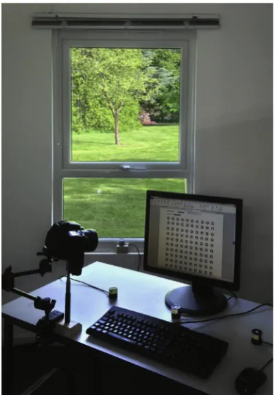
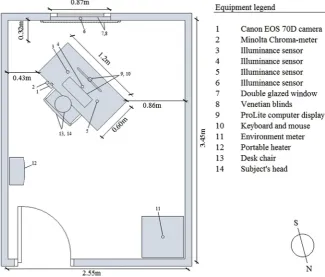
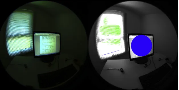
To investigate temporal effects on glare response from daylight, an experiment was designed using a test room provided with a window and a view to an external natural scene (Fig. 1).

Forty subjects participated to the experiment, which was carried out between the months of March and April, a period of mixed weather varying from overcast to clear skies. Subjects were recruited by purposive sampling via an online advertisement. No criteria were used for the exclusion of volunteers. Participants were all postgraduate students, 12 male and 28 female, varying in na-tionality and cultural background (20 white, 17 Asian, 1 mixed, and 2 other), the mean age was 25.00 (SD¼2.59), 3 left-handed, 37 right-handed, 15 wore corrective lenses, and all were self-certified as having no other eye problems.

The test room was located at the University of Nottingham, UK (latitude: 525601900N; longitude: 11104200W), and had internal di-mensions of 3.45 m 2.55 m and a ceiling height of 2.35 m. It featured a south-east facing window (azimuth¼165) of 0.87 m width and 1.47 m height. The room surfaces had reflectance properties of:

rwall

¼0.6,

rceiling

¼0.8,

r

_floor¼0.2. The window was

equipped with user-controlled venetian blinds mounted on the internal wall. Each slat of the shading system was convex in shape, with dimensions of 110 cm2.5 cm, and a distance of 2.5 cm between each slat. The slats were white in colour, with reflectance

of:

rupper

¼0.90 and

rlower

¼0.72. A workstation (desk, chair, and

desktop computer) was placed inside the room at a 45position from the window. The surface of the desk had reflectance of

r

¼0.42, dimensions of 120 cm60 cm, and a height of 72 cm from thefloor. Aflat screen 1900iiyama ProLite B19065 liquid crystal display (mean self-luminance ¼201.64 cd/m2) was used as the Visual Display Unit (VDU) to present a series of visual tasks to test subjects (Fig. 2).

A diagonal arrangement of the workstation was selected instead of a desk positioned parallel or perpendicular to the window, since previous studies conducted under similar layouts found that, when asked to provide a glare assessment, subjects would often deviate their sight from the display and look at the window, while photo-metric instruments would capture the luminous condition of the VDU[5,15,16]. Conversely, a desk positioned 45clockwise from the window allowed to mitigate the risk of unwanted head movements between the VDU and the window when glare assessments were made.

The selection of the desk position was also confirmed by a pilot study (N¼10), where a parallel and a diagonal arrangement of the workstation were explored. Coherent with the literature[5,15,16], it was observed that, under the parallel position, subjects would often look directly at the window when asked to provide a glare assessment, while this behaviour was less apparent with the desk placed diagonally. Also, under the parallel set up, there was an unwanted visual parallax effect associated with the location of the workstation, such that the computer screen would partially obstruct certain parts of the window view. These unwanted effects could be minimised under the diagonal arrangement.

The experimental procedure requested subjects to participate to three test sessions, whose order was randomised over three consecutive days, distributed at 3-h intervals:

Morning: 09:00 or 09:30

Midday: 12:00 or 12:30

Afternoon: 15:00 or 15:30

At each test session, subjects were asked to perform two series of three visual tasks [17]. Each series was completed under a different shading setting: adefaultshading, with blinds set at a cut-off slat angle that ensured predominantly diffuse daylight condi-tions, yet allowing a perception of the external view; and auser-set

shading, where blinds were adjusted to the subject's own prefer-ences (Fig. 3).

The procedure was consistent with the laboratory tests described in Kent et al.[11,14]and Altomonte et al.[12], although the evening session (18:00 or 18:30) was excluded from this study due to seasonal variation in day length and sunset occurring before its starting time.

During the tests, subjects were asked to make glare assessments using as benchmarks the adaptations of Glare Sensation Votes (GSVs) used by Iwata et al.[18,19], Iwata and Tokura[20], and Mochizuki et al. [21]. These glare criteria correspond to the sensation of visual discomfort experienced:‘Just (Im)Perceptible’,

‘Just Noticeable’, ‘Just Uncomfortable’, and ‘Just Intolerable’. To reduce the risk of self-interpretation, and ensure that the GSVs could be understood by subjects according to the intentions of the experimenter [1], each criterion was linked to a time-span descriptor[22,23].

[image:2.595.58.258.436.724.2]

In the selection of the GSV scale it was considered that, when forcing a continuous dependent variable (e.g., a glare index) into discrete categories associated with subjective levels of glare sensation (i.e., the 4-point GSV scale), there is a risk of uninten-tionally making respondents report a stimulus that does not accurately reflect their perceived evaluation of that stimulus [1].

However, according to the literature[24,25], a multiple criterion technique of subjective appraisal should be preferred over a forced-choice dichotomous scale (e.g., yes/no, comfortable/uncomfortable) when evaluating individual differences from glare sensation. Also, when the number of possible outcomes becomes too large, further sources of bias might be potentially introduced through self-interpretation or the abstraction caused by similarities in the se-mantic meaning of categories anchored to the scale (i.e., it may not be easy to discriminate distances between benchmark labels)[26]. For this reason, the 4-point GSV scale was preferred over the 9-point multiple criterion technique scale used by other researchers

[2,3,18e20,22,23]. Similar adaptations have also been used in other previous studies[15,27].

Before the subjects entered the test room, the venetian blinds were adjusted at the default cut-off position in response to external

conditions in order to ensure that no direct sunlight was present in thefield of view of the observer during thefirst part of the test[16]. At the beginning of theirfirst test, subjects were required to position themselves at the desk facing the computer screen. A set of instructions was then given, including a definition of discomfort glare, the meaning of each GSV criterion and time-span descriptor, and an illustration of how the experiment would run. At this point, subjectsfilled in a short questionnaire featuring demographic in-formation (age, gender, ethnicity, etc.) and self-assessment of per-sonal factors (e.g., chronotype, photosensitivity). Participants were then required to trial a series of simplified visual tasks to familiarise themselves with the test procedure. Thefirst consisted in a‘landolt ring’pre-test, whereby subjects looked at a chart and counted the number of rings that had a gap in a specified orientation[5,28]. In the‘letter searching’pre-test, subjects looked at a short

[image:3.595.139.465.68.345.2]

pseudo-Fig. 2.Layout of the test room and list of equipment.

[image:3.595.147.464.382.544.2]

text and counted the number of times a specific letter appeared

[16]. Finally, the‘typing’pre-test consisted of a short pseudo-text that had to be manually typed into a space on the computer screen [9,16,17]. All trial tasks were presented on the VDU. Following the completion of each pre-test task, using a GSV scale displayed on the screen, subjects were asked to indicate their perceived magnitude of glare sensation given by the daylight coming from the window. At this point, the experimenter collected a series of seven Low Dynamic Range Images (LDRI) with varying exposure values, and a single vertical illuminance measurement. All data from the pre-test were recorded but were not included in the main analysis. The pre-test was followed by a brief relaxation period (1e2 min), whereby any further questions could be clarified. At the end of the pre-test, the full experimental procedure started. Extended versions of the same visual tasks were used during the experimental stage, and were presented under a randomised sequence. Since the procedure used a repeated-measure design, these tasks have been selected to minimise the risk of unwanted carry-over effects (e.g., learning), which could have occurred if normal text (i.e., newspaper articles) had been used[29]. Moreover, it was not considered feasible to provide letter searching and typing tasks with content that was both independent from one another and homogenous enough for a within-subject analysis. Instead, pseudo-textsefeaturing random letters with upper and lower case and numbers e prevented repetition of identical stimuli, while retaining the experimental integrity needed for statistical analysis

[30,31]. The likelihood of carry-over effects was further reduced by randomising the content of the pseudo-texts used for each task. In addition, since differences in perceived visual discomfort have been associated to a variation in difficulty of the task due to a change in size, contrast, or background of the text [12,32,33], the effect of visual task difficulty was controlled by presenting characters al-ways set at Arial, 12-point size, with black font colour on white background, and at 2.0 line spacing.

The experimental procedure followed the same methodology of the pre-test, with subjects performing the three visual tasks, expressing their vote of glare sensation after each task, and photometric measurements being taken after every glare assess-ment. Once thefirst series of three tasks was concluded with the shading device maintained at a default cut-off position, subjects were asked to adjust the venetian blind slats to their preferred configuration, and the procedure was repeated with three more visual tasks presented in a randomised order (Fig. 4).

At the end of each test session, subjects were requested tofill-in afinal short questionnaire, providing self-reports of several tem-poral variables: fatigue, hunger, caffeine intake, mood, prior light exposure, and sky condition. The entire session lasted around 25e30 min.

2.2. Photometric measurements and glare indices

The experimental procedure adopted in this study involved drawing a relationship between personal glare judgements and objective photometric quantities[22,23]. This required the partic-ipants to evaluate their visual conditions using subjective assess-ment methods, and then combining votes of glare sensation with simultaneous measurements of the luminous environment.

Three photometric instruments were used to‘instantaneously’

capture the luminous environment of the observer: 1) a Charge-Coupled Device (CCD) camera equipped with afish-eye lens; 2) an illuminance chromameter; and, 3) a series of horizontal minance sensors connected to a data-logger. The camera and illu-minance chromameter were mounted on the desk and pointed towards the VDU, which was assumed to be the visualfixation area. They werefixed on adjustable arms to be as close as possible to the

observer's head without causing visual impairment or distraction

[5](Fig. 5).

The CCD camera was a Canon EOS 70D equipped with a 4.5 mm f/2.5 EX DC GSM 180Sigmafish-eye-lens mounted on a Monfrotto extendable arm. CCD devices utilise conventional photographic techniques to obtain photometric measurements. In other words, pictures taken by CCD cameras can be used for deriving luminance values, which are contained within the scene pixels corresponding to different points of measurement in the captured scene[34,35]. The quality of the images taken with the CCD camera depends on both the aperture (f/N, whereby the f-number is the ratio between the lens's focal length and the entrance diameter) and the time during which the shutter is open (exposure time, (v)). At a constant focal length, the aperture becomes proportional to the square of its value (1/f2). The combination of both settings is often referred to as image quality, or exposure value, and is proportional to v/f2. Therefore, if the sensitivity (ISO) and gain (whereby, the gain is the ratio between the number of photoelectrons received by the CCD and the number of pixels within the captured image) of the camera sensor are constant, the quality of the image produced by the CCD is solely proportional to v/f2(i.e., the exposure time and aperture) and can be fully expressed using (Eq.(1))[36]:

EV¼3:32log10

f2 v

(1)

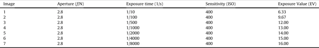
In this study, for each photometric measurement, seven inde-pendent Low Dynamic Range Images (LDRI) were taken with the camera, using varying Exposure Values (EVs) to capture the full range of luminance variation within thefield of view[32].Table 1

presents the properties of the LDRI images used for this investi-gation, indicating the corresponding camera settings in terms of aperture (f/N), exposure time (1/s), sensitivity (ISO), and exposure value (EV).

The LDRI images were combined into a Radiance-formatted High Dynamic Range Image (HDRI) using the ‘data fusion’ soft-ware Photosphere[37], which merges several LDRIs into a single HDRI [38]. The HDRI images could then be evaluated using the Evalglare tool version 1.11[17]. Once the images were combined, the camera response function_e a regression curve showing the relationship between a luminance value and a pixel within the image ewas computationally derived through a self-calibration process using a spot-point measurement taken with a Minolta LS-100 luminance meter.

The second photometric instrument was a Minolta chroma-meter CL-200a mounted vertically on the desk, adjacent to the camera[16,17]. This was used to independently take vertical illu-minance measurements to be compared with the illuillu-minance values calculated by Evalglare for each luminance image taken by the CCD camera. Therefore, a comparison could be made between the light reaching the sensor of the chromameter and that entering the lens of the CCD camera.

The last photometric instruments were represented by three horizontal illuminance sensors that were distributed evenly at a distance of 20 cm from each other on the desk, and one horizontal illuminance sensor placed centrally on the internal window sill. These sensors were connected to a data-logger that recorded hor-izontal illuminance every 10 s[16].

To check the integrity of photometric values obtained from the instruments, a comparison was made between the vertical illumi-nance measured by the chromameter and the illumiillumi-nance calcu-lated by Evalglare from the CCD camera images, under the default and the user-set shading settings (Fig. 6).

hypothesis diagonal line can be accounted for by the slightly different position of the camera lens and the chromameter[16]. Larger differences could be due to direct sunlight transmission through gaps in the blind slats that, in some cases, might have hit the camera lens but not the illuminance sensor. However, these differences are not to be regarded as problematic[17].

To provide a more rigorous comparison, the Mean Absolute Deviation (MAD) and the Root-Mean-Square-Error (RMSE) were calculated for the illuminance values calculated from the CCD

images and those measured by the chromameter based on (Eq.(2)) and (Eq.(3))[39,40]:

MAD¼ _N1 Xn

i¼1

jECCD ECMj (2)

Introduction

Questionnaire (demographic, personal factors) Pre-test

Landolt ring taska (3 minutes)

Glare assessments and photometric measures Letter searching taska (3 minutes) Glare assessments and photometric measures Typing taska _{(3 minutes)}

Glare assessments and photometric measures

Landolt ring taskb _{(3 minutes)}

Glare assessments and photometric measures Letter searching taskb _{(3 minutes)} Glare assessments and photometric measures Typing taskb (3 minutes)

Glare assessments and photometric measures Questionnaire (temporal variables)

Additional questions

a, b _{Visual tasks (landolt ring, letter searching, typing) were presented to test subjects under a randomised order}

End of experiment

Adjustment of shading device (default)

Adjustment of shading device (user-set) Start of experiment

Default shading setting Duration: approximately 10 minutes

[image:5.595.123.481.64.279.2]

User-set shading setting Duration: approximately 10 minutes

[image:5.595.143.459.325.485.2]

Fig. 4.Experimental procedure.

Fig. 5.Photometric instruments.

Table 1

Properties of the LDRI images.

Image Aperture (f/N) Exposure time (1/s) Sensitivity (ISO) Exposure Value (EV)

1 2.8 1/10 400 6.33

2 2.8 1/100 400 9.67

3 2.8 1/500 400 12.00

4 2.8 1/1000 400 13.00

5 2.8 1/2000 400 14.00

6 2.8 1/4000 400 15.00

[image:5.595.43.561.541.619.2]

RMSE¼

ffiffiffiffiffiffiffiffiffiffiffiffiffiffiffiffiffiffiffiffiffiffiffiffiffiffiffiffiffiffiffiffiffiffiffiffiffiffiffiffiffiffiffiffiffi 1

N

XN

i¼1

ðECCD ECMÞ2

v u u

t ₍₃₎

where, ECCDis the illuminance calculated from the CCD images and

ECMis the illuminance measured by the chromameter.

The MAD and RMSE are estimates of the average error expressed in the units of the variable of interest (i.e., lux)[39,40]. The MAD measures how two data sets are likely to differ from their mean by taking their average absolute value (ECCDeECM). This is to prevent

differences with opposing signs from cancelling each other out. The RMSE is a measure of the deviation, on average, of a data point from the null hypothesis line[41].

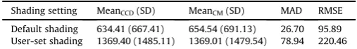
For the full set of data under both shading settings, Table 2

displays the mean and standard deviation (SD) for the illumi-nance values calculated from the CCD images (MeanCCD) and those

measured by the chromameter (MeanCM), the MAD, and the RMSE.

The results indicate that the average errors, both MAD and RMSE, are lower under the default shading setting. As per the graphical observations, this suggests that the differences between calculated and measured illuminance values were smaller when blinds were set at their default position.

A range of photometric measures and glare indices were collected and calculated to select an evaluation parameter that would be appropriate to test the postulated temporal effects on glare response from daylight. These included: illuminance at the eye obtained from Evalglare (Eeye); illuminance at the window sill

(Esill); luminance of the source (Lsource); average luminance (Lavg)

(this being the average luminance within a given HDRI scene evaluated by Evalglare); Daylight Glare Probability (DGP) [16]; Daylight Glare Index (DGI)[42,43]; Unified Glare Rating (UGR)[44]; and, CIE Glare Index (CGI) [45]. Rather than independently reporting the statistical and practical significance of the effect of experimental interest using each of the photometric values and glare indices above, all outcomes corresponding to the different times of day were plotted onto a product-moment correlation matrix. The matrix uses the Pearson's correlation coefficient r as a measure of the strength of the relationship that exists between variables [41]. The Pearson's matrix showed that all correlations between photometric values and glare indices were statistically

significant and with substantive effect sizes, the only exception being for the Esill, which presented a weak association to other

variables. Therefore, it was inferred that, across the times of day, there was a strong correlation between measured photometric values (excluding the Esill), those calculated by Evalglare, and the

glare indexes considered; hence, a single metric could be sufficient to evaluate the effect of experimental interest.

To identify the metric most suitable to this analysis, reference was made to a study by Wienold[17], who detected statistical significance when several photometric values (e.g., illuminance at the eye, average image luminance, etc.) and glare indices (Daylight Glare Probability (DGP), Daylight Glare Index (DGI), etc.) were used to predict the possibility that an observer would be disturbed by glare from a window. Out of these metrics, the DGP was charac-terised by the strongest correlation with the probability of glare occurrence. Also considering that other indices (e.g., Unified Glare Rating and CIE Glare Index) have not been designed to deal with non-uniform sourceseas, for example, caused by venetian blinds, luminance variations within a given view (e.g., due to the ground, buildings, variation in cloud cover)[3,16], or small sources sub-tending a solid angle below 0.01sr[46,47]ethe DGP (Eq.(4)) was selected as the evaluation parameter for this study:

DGP¼5:87$105$Evþ9:18$102$log 1 þ X

i L2

s;i $

u

s;i E1:87

v $P2i

!

þ 0:16

(4)

where, Ev is the vertical illuminance at the eye (lux), Ls is the

luminance of the glare source detected by Evalglare (cd/m2),

us

is the subtended size of the source (sr), and Piis the position index [16].

The DGP provides an indication of the percentage of people that would be disturbed by the daylight glare present within thefield of view[17]. Unlike other glare indices, the DGP is mainly dependent on the vertical illuminance at the eye, since the remaining factors within the formulaeLs,

us

, and Pi,ehave smaller weighted terms [48].

2.3. Size and position of the glare source

The glare search algorithm adopted by Evalglare uses a task definition criterion whereby afixation area covering most of the VDU is outlined within the image (the blue circle inFig. 7).

[image:6.595.93.492.66.198.2]

If no clearfixation area is present in the scene (this was not the case in this study), Evalglare reverts to a default detection method by: calculating the average luminance of the entire image and

Fig. 6. Comparison between calculated (from the CCD images) and measured (from the chromameter) vertical illuminance values, for the default (left) and user-set (right) shading settings.

Table 2

Descriptive analysis of calculated (CCD) and measured (CM) illuminance values.

Shading setting MeanCCD(SD) MeanCM(SD) MAD RMSE

[image:6.595.31.285.706.741.2]

treating as a glare source every pixel with a luminance valuex-time (sensitivity parameter) higher than the scene average; or, taking a

fixed value of luminance and treating every pixel that has higher luminance than this as a glare source[17]. The sensitivity param-eter for the search algorithm is recommended to be within 2e7 times the average task or scene luminance, although this is part of ongoing research[48]. For this study, each pixel with a luminance value exceeding by more than 5 times the average luminance of the defined task-zonefixation area was treated by Evalglare as a glare source. This implies that, in the assessments made by Evalglare, the glare source might not necessarily correspond to the window area (Figs. 8 and 9; the colours of the glare sources are arbitrarily set by the tool, without being linked to glare magnitude).

When evaluating the HDRI images at each test session and time of day, it was noted that the size and position of the glare sources detected by Evalglare varied under all shading settings. This pre-sented a problem since the literature suggests that the magnitude of glare sensation can be influenced by both the size[13]and the position of the source relative to the line of sight[49].

Consistent with the literature[3,50], to address this issue, rather than measuring and controlling for the size and the position indices of the individual glare sources independentlyewhich, in the DGP formula, are computed as distinct factors e the solid angle (

u

) subtended by the glare source modified by the position index (P) was used as a covariate, since it is a combination of both parame-ters. Hence, by only controlling for the effect of one variableei.e., the solid angle subtended by the glare sources modified by the position index (denoted by

U

)e high statistical power could be retained in the analysis. Also, the distortion associated with the

‘nuisance’variable could be removed[41]. This enabled to reduce

the total amount of error and allowed to isolate the effect of experimental interest with greater accuracy[51]. Conversely, failing to account for confounding variables would have inflated uncer-tainty within the estimates associated with point values (i.e., mean, variance, and confidence intervals)eincreasing the risk of occur-rence of Type I errors_eand, as a consequence, might have led to inaccurate conclusions[52,53].

2.4. Statistical analysis

2.4.1. Multilevel modelling

A multilevel model (MLM) with fixed effects (i.e., changes in independent variables associated with variations in the evaluation parameter or dependent variable) was initiallyfitted to compare the DGP values for all variables that were experimentally manip-ulated against each other, while controlling for the effect of glare source size and position. The specifiedfixed effects were:

Time of day;

Shading setting;

Task type;

Glare Sensation Vote (GSV).

[image:7.595.148.463.67.226.2]

The MLM was selected for this study since it is a statistical method suitable to analyse data with complex structures[54]. The main difference between multilevel and unilevel models (e.g., t-tests, ANOVA, etc.)ewhich test the variation caused by a single (unilevel) effect by making comparisons between two or more in-dependent variableseis that, in MLM analysis, the independent variables are nested in a model with multiple levels (or effects)[55].

Fig. 7.HDRI with Radiance formatting (left); Evalglare image with task definition (right).

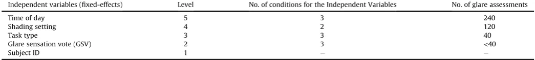
[image:7.595.134.474.604.720.2]

[image:8.595.121.463.67.182.2]

Table 3displays the independent variables under examination (specified asfixed effects), the level in the MLM model where each variable is located, the number of conditions (independent groups) for each independent variable, and the number of glare assess-ments collected for each condition group.

For example, for the fixed effect‘Time of Day’ (level 5), the number of glare assessments collected for each condition (i.e., test sessions) is the highest, since the total number of glare assessments (N¼720; that is, 40 subjects providing glare assessments at 3 times of day after performing 3 visual tasks under 2 shading settings) is divided by three independent conditions (Morning, Midday, and Afternoon). For level 2,_‘Glare Sensation Vote (GSV)_’, the number of glare assessments collected for each outcome variable is the lowest, since the number of glare assessments is divided by the number of condition groups at that level, in addition to all the condition groups that exist within the independent variables located at higher levels within the model.‘Subject ID’is featured at the bot-tom of the model (level 1), representing personal regression slopes associated with each subject, which allows the MLM to distinguish within-subject variance from between-subject variance[41,56].

In this analysis, the GSV was specified as afixed effect, although this could have been also classified as a random effect[51]. In the latter case, any variation on the reported GSV would have not been considered as occurring due to experimental manipulation, but rather to dynamic changes in the environmental conditions or to variables that are personal to the test subject. However, the liter-ature suggests that, in multilevel modelling, a variable should be specified as afixed effect (rather than a random effect) if it is of primary experimental interest [57]. In previous studies

[2,3,5,16,17,22,23], reported levels of glare sensation have effec-tively always been treated asfixed effects.

The MLM analysis postulates that the glare assessments recor-ded in each of the upper level measurements (levels 2, 3, 4, and 5) should be correlated both within each level (e.g., time of day) and across each of the multiple levels (for example, time of day and shading setting). In other words, since test subjects were requested to provide votes of glare sensation on multiple occasions, at each level within the model and for each condition group, there is a relationship between reported levels of GSV. This relationship,

however, causes a lack of independence between observations that are clustered on multiple levels, which has to be properly addressed as explained below[58,59].

2.4.2. Independence of observations

In the analysis of the data, it was considered that glare assess-ments might not have been independent from each other[60]. To examine whether the assumption of independence had been satisfied, the intra-class correlation (ICC) was calculated according to the following formula (Eq.(5)):

ICC¼

t

00

t

00þ

s

2

(5)

where,

t

00 is the estimated variance (i.e., the variation in DGP

values at levels 2, 3, 4, and 5 (within-group variance)) and

s

2_{is the}

residual variance (i.e., the variation in DGP values at level 1 (be-tween-group variance))[55,61].

Utilising Eq.(5), the ICC calculated for the full set of data was: 0.002577/(0.002577þ0.000340)¼0.883442. This outcome was measured by the benchmarks provided by Julian [58] for low, moderate, and large ICCs (ICC0.05, 0.15, and 0.45, respectively), indicating a large intra-class correlation (ICC>0.45). This suggested that the assumption of independence had not been satisfied.

In interpreting this result, it was considered that MLM are tests that account for dependencies among observations that occur at multiple levels[60]by estimating a single variance structure that represents how spread-out the random intercepts are around the common intercept of each group[56]. In other words, the covari-ance structure estimates how the varicovari-ance parameters for each subject are related across thefixed effects within the MLM[62], and compares this to a specified covariance structure using a goodness-of-fit index[41]. This effectively relaxes the assumption of inde-pendence within the inferential test [62]. Therefore, it can be concluded that multilevel modelling is an appropriate statistical method of analysis when the assumption of independence has not been satisfied[41,59,61,63,64], reinforcing the reasons behind its selection for this study.

[image:8.595.31.554.249.308.2]

Fig. 9.Examples of task zone (blue circle) and glare sources detected by Evalglare at the Morning (left), Midday (middle), and Afternoon (right) test sessions under the user-set shading setting. (For interpretation of the references to colour in thisfigure legend, the reader is referred to the web version of this article.)

Table 3

Distribution of glare assessments across independent variables (fixed effects MLM).

Independent variables (fixed-effects) Level No. of conditions for the Independent Variables No. of glare assessments

Time of day 5 3 240

Shading setting 4 2 120

Task type 3 3 40

Glare sensation vote (GSV) 2 3 <40

2.4.3. Covariance structure and goodness-of-fit

Multilevel modelling offers a flexible approach to estimate variance parameters, since direct assumptions regarding covari-ance structure (i.e., how the varicovari-ances associated with each inde-pendent group are related to each other) can be specified[54]. This assumption depends on experimental design; for example, in time-based studies, the variance associated with independent groups may change due to experience and practice effects [42]. In this study, an autoregressive (AR(1)) covariance structure was adopted within the variances associated with each independent group. In fact, measurements taken at closer time steps were postulated to be more highly correlated than for longer intervals[56]. Hence, it was assumed that variances systematically changed over time[41].

To assess the suitability of the covariance structure applied to the MLM, a goodness-of-fit index can be calculated. This index as-sesses the overallfiteusing a

c

2likelihood ratio testebetween the estimated variance parameters and the selected covariance struc-ture. The literature recommends that the Bayesian Information Criterion (BIC) is used, which adjusts the statistical outcome based on the number offixed effects and the sample size used within the MLM[41,56]. In interpreting the outcome of the BIC, the smaller the value (

c

2), the better the modelfit. However, no absolute inter-pretation can be made of the statistical outcome; that is, no conclusive information can be inferred from this single statistical value[41]. Instead, the BIC can be compared to equivalent values from other models that contain either additional random effects (retaining the original MLM with_fixed effects) or use a different covariance structure[56]. Therefore, by increasing the complexity of the model (e.g., by including additional random effects), the BIC provides statistical information that can be used to estimate the presence of unknown parameters within the MLM.

2.4.4. Significance testing and estimates of covariance parameters

For eachfixed effect, the main interaction was tested by ana-lysing the significance of the difference between two or more means at a single levelee.g., for level 5‘Time of day’: Morning vs. Middayewithout grouping the dependent variable (DGP) by other

fixed effects. In addition, interactive effects between thefixed ef-fects and the covariate (i.e., the solid angle subtended by the glare source modi_fied by the position index (

U

)) were speci_fied for in-clusion in the inferential analysis. This required testing the signif-icance of the differences between two or more means across independent variables (e.g., level 5 _‘Time of day_’ and level 4

‘Shading setting’).

In the MLM, all possible outcomes on the dependent variable (DGP) were specified using the variables known to vary within the experiment (i.e., time of day, shading setting, task type, and GSV). This was assumed to‘consume’as much as possible of the scatter commonly associated with subjective evaluations of glare sensation

[13]. In essence, the MLM was used to analyse whether there was sufficient evidence in the data from the test room experiment to infer that, at different times of day (Morning, Midday, and After-noon), mean DGP values corresponding to equal reported levels of glare sensation were statistically (significance testing) and practi-cally (effect size) different from each other. This would allow sub-stantiation of earlier _findings [11,12,14] and provide statistical evidence of the postulated temporal effects on glare response from daylight.

All outcomes on the DGP were specified in the MLM using the

fixed effects available (main interactions and interactive effects). The MLM analysis provides estimates of mean parameters and their associated statistical difference. When a statistically significant difference is detected, there is a reduction in the total amount of variance present within the model[56]. Once all mean parameters have been estimated, the MLM calculates whether the remaining

unexplained variance is signi_ficantly different from a model that has variance equal to zero; this test is called the Wald Z statistic

[61].

The statistical power of the Wald Z statistic depends on the size and evenness of the sample and, more importantly, on the number of interactive effects within the model[64]. The more interactive effects are specified, the smaller the estimated variance parameter becomes. The null hypothesis is that the unexplained variance within the model is equal to zero[56]. As an alternative hypothesis, the Wald Z test seeks to demonstrate that there is sufficient evi-dence from the data to infer that the unexplained variance is not equal to zero and that, therefore, there are other unmeasured variables that are unaccounted for within the MLM.

2.4.5. Parameter estimation

Two methods can be used for parameter estimation in multi-level modelling: Maximum Likelihood (ML) and Restricted Maximum Likelihood (REML). The ML provides more robust esti-mates offixed regression parameters[41], although this method is dependent upon large sample sizes[61,64]. This limitation is not problematic for main interactions or interactive effects (i.e., the influence of multiple fixed effects on the dependent variable). However, when the sample size becomes low due to the number of levels within the MLM, parameter estimates may not be robust[65]. This is one of the disadvantages behind the use of MLM analysis, since the sample distribution will always be lowest at the group level[63]. In addition, the major caveat of multilevel modelling is that different models can only be comparable if ML estimation has been used[41]. For this reason, the Maximum Likelihood method was adopted for this analysis.

3. Results

3.1. Fixed-effects multilevel model

Table 4provides descriptive and inferential statistical values for the photometric and physical parameters measured throughout the experiment. The table presents the vertical illuminance, the source luminance, and the glare source size and positionecalculated from the HDRI images and analysed using Evalglare_efor the three times of day and the two shading settings featured in this study. Since the horizontal (desk) illuminance and the vertical illuminance received at the CCD camera's lens were strongly correlated _e N _¼ 720,

p0.001, r¼0.71eonly the vertical illuminance has been re-ported in the table. For each variable and under each shading setting, the table displays the marginal mean of the corresponding measurement parameter, the standard error, the degrees of freedom (df), and the lower (CUL) and upper (CIU) confidence

in-tervals for the marginal mean values as calculated by the multilevel model with ML estimation. The table shows that the mean average values and the lower and upper confidence intervals of the source luminance e corresponding to the detected glare pixels with luminance exceeding by more than 5 times the average luminance of the defined task-zonefixation area[17]eare relatively consis-tent across times of day and shading conditions. Conversely, for the same glare pixels, the mean values of the vertical illuminance and of the glare source size and position vary significantly (p0.001), as indicated by the MLM analysis.

Intolerable’were reported, these criteria were merged to perform meaningful statistical analysis[5].

Under the default shading setting, the displays suggest a consistent trend for central tendencies to correspond to increasing levels of DGP for each GSV criterion as the day progresses. It is worth reminding that a larger DGP signals a higher probability that an observer may be disturbed by the glare source. Since each re-ported vote of glare sensation (e.g., Just (Im)Perceptible) corre-sponds to increasing mean values of DGP along the day (from Morning to Midday to Afternoon), the plots suggest thatewhen the blinds were set at their default positione subjects showed higher tolerance to the combination of photometric and physical parameters associated with the glare source once providing their assessment at later test sessions (i.e., the same GSV was given un-der conditions characterised by higher probability of glare occur-rence). If substantiated by inferential testing, this would support an effect of time of day on glare response, as detected in previous laboratory experiments[11,12,14].

Under the user-set shading setting, this tendency is not

apparent. In fact, in this case, visual inspection of statistical pa-rameters shows no prevailing tendency for any of the GSV criteria as the day progresses. Therefore, there is no graphical evidence to suggest that an effect of time of day was present on glare response when subjects were allowed to control the setting of the venetian blinds.

Initial inferential analysis of the data detected no statistically significant difference for the (main and interactive) effect of task type on glare response:F(2, 670.76)¼0.19,p¼0.83. Therefore, task type was excluded from any post-hoc analysis in order to reduce the number of levels within the model and prevent the occurrence of Type II errors[56].

[image:10.595.40.530.83.504.2]

For every test, the DGP was calculated at a constant value of the solid angle subtended by the glare source modified by the position index to control for its temporal influence on the dependent vari-able (

U

¼0.27). This value (

U

) was defined by the statistical package (SPSS) and was an adjustment derived from the MLM through multiple regression, utilising the alpha-level (statistical signi_fi -cance), the coefficient of the outcome (i.e., the mean difference in

Table 4

Descriptive and inferential statistical values for the photometric and physical parameters.

Variable Time Shading Mean Std. error df CIL CIU

Vertical illuminance [lux] Morning Default shading 603.66 134.77 236.18 338.15 869.17

User-set shading 1412.31 182.00 503.57 1054.74 1769.88

Midday Default shading 1077.36 136.99 250.77 807.57 1347.15

User-set shading 2039.60 150.28 335.14 1743.99 2335.21

Afternoon Default shading 446.17 132.79 226.14 115.50 707.84

User-set shading 862.41 160.05 334.20 547.61 1177.22

Source luminance [cd/m2_{] Morning Default shading 1789.06 336.23 224.81 1126.49 2451.62}

User-set shading 5068.47 445.13 477.90 4193.82 5943.13

Midday Default shading 2183.56 341.22 237.69 1511.36 2855.76

User-set shading 5064.34 371.55 313.66 4333.31 5795.38

Afternoon Default shading 1755.50 331.68 215.68 1101.76 2409.24

User-set shading 4328.80 395.36 326.70 3551.03 5106.57

Glare source size and position [U] Morning Default shading 0.24 0.03 179.03 0.18 0.31

User-set shading 0.44 0.04 352.70 0.36 0.52

Midday Default shading 0.33 0.03 186.10 0.26 0.39

User-set shading 0.38 0.03 230.69 0.31 0.45

Afternoon Default shading 0.05 0.03 173.35 0.01 0.10

[image:10.595.121.468.270.502.2]

User-set shading 0.18 0.04 251.76 0.11 0.26

DGP calculated from the HDRI images evaluated by Evalglare) weighted for the effect of the covariate (i.e., the solid angle sub-tended by the glare sources modified by the position index calcu-lated from the images evaluated by Evalglare) regressed onto the

fixed effects (i.e., time of the day), and the unexplained residual variance remaining within the model[41,51].

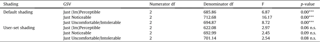
Univariate tests were then performed, grouping the effect of time of day by the reported GSV and by shading setting. These tests compared the DGP at all times of day, similar to an Analysis of Variance (ANOVA). Table 5shows the inferential data from the univariate tests (fixed-effects MLM), providing the shading setting, the GSV criteria, the degrees of freedom (df), the test statistic (F), and the statistical significance (p-value).

The univariate tests showed that, under the default shading setting, the variations of DGP values at different times of day were all statistically significant. However, when the blinds were adjusted by subjects, no significant evidence was detected of an effect of time of day for any of the GSV criteria.

To isolate the main effects between variables, contrasts were made using pairwise comparisons[66], whereby all permutations between times of day were compared against each other. The directionality of the hypothesis was informed by examination of descriptive statistics and visual inspection of central tendencies from graphical displays [67]. Since no consistent directionality between observed differences could be detected when considering both shading settings, two-tailed hypothesis testing was adopted

[68]. In consideration of the experiment-wise error rate caused by the significance level inflating across multiple tests carried out on the same hypothesisecalculated as 1-(0.95)n¼0.14 (thus, risking a 14% probability of making at least one Type I error), where n¼3, i.e. the number of pairwise comparisons performedeBonferroni cor-rections were applied[69]. As null hypothesis significance testing (NHST) depends both on the size of the sample and on the magnitude of the effect under examination[70], emphasis of the inferential tests was placed on the effect size (i.e., a standardised measure of the observed difference between groups) and not solely on their statistical significance (which, particularly for small or uneven samples, could confound effect size and sample size)

[71,72]. The effect size was calculated by the Cohen's d coefficient, according to the formula (Eq.(6))[73]:

Cohen0s d¼

_s

D

M

pooled

(6)

where,

D

M is the difference between the estimated marginal means and

s

pooledis the pooled standard deviation adjusted for the

effect of glare source size and position by the MLM analysis. The interpretation of the outcomes derived from the conserva-tive benchmarks provided by Ferguson[74] for small, moderate, and large effect sizes (d0.41, 1.15 and 2.70, respectively). Values below 0.41 were not considered to be substantive (i.e., they were deemed non-practically relevant effects).

For each GSV criterion,Table 6provides the shading setting, the

times of day, the number of glare assessments (N) reported by test subjects (x0and x1corresponding to the test sessions considered in

the pairwise comparisons), the difference between the estimated DGP marginal means (

D

M) and its associated two-tailed statistical significance (NHST,p-value with Bonferroni correction), the stan-dard error, the degrees of freedom (df), the lower (CIL) and upper

(CIU) 95% confidence intervals for the difference between marginal

means, and the effect size (d).

Under the default shading setting, analysis of descriptive and inferential statistics showed that mean differences (

D

Ms) and effect sizes (d) were consistently negative, hence signalling higher values of DGP at later test sessions for each GSV. The

D

Ms were highly significant in 4 cases, significant in 2 cases, weakly significant in 1 case, and not signi_ficant in 2 cases. All differences detected had a substantive effect size (Cohen's d absolute value: 0.41d<1.15). Inferential results from thefixed-effects MLM under the default shading setting, therefore, confirmed the hypothesis of a tendency for the DGP to increase as the day progresses for all the criteria of glare sensation.

Under the user-set shading setting, no consistent directionality of the sign could be observed for descriptive statistics (

D

Ms),

con-fidence intervals, and effect sizes. The pairwise comparisons detected no statistically significant differences, with effect sizes that were practically relevant (d0.41) only in 3 cases. Therefore, for the user-set shading, thefixed-effects MLM did not support the postulation of an effect of time of day on reported glare sensation from daylight.

Based on these inferential results, further analysis was con-ducted to investigate whether, in the multilevel model, there was evidence to suggest that thefixed effects alone were not sufficient to explain the variance present within the data. The estimates of covariance parameters showed a highly significant difference (Wald Z¼12.28,p0.001), hence confirming that the unexplained variances within the model were not equal to zero. This led to the hypothesis that there might be other variables influencing the spread in glare response that were beyond the specifiedfixed ef-fects, suggesting that random effectsein this case, the self-reports of temporal variables provided by test subjects at each test session

eneeded to be included in the MLM[51,55].

3.2. Mixed-effects multilevel model

To include consideration of temporal variables in the analysis, a mixed-effects MLM withfixed and random effects was fitted in order to compare the DGP values for the times of day, shading setting, and GSV against each other, while controlling for the effect of glare source size and position.

[image:11.595.43.563.664.733.2]

In a mixed-effects MLM,fixed effects are generally factors that do not change across individuals or that can be manipulated from the experimenter, while a random effect is likely tofluctuate be-tween test subjects[41]. A variable is specified as afixed effect to take into consideration the variability caused by the same partici-pant across various conditions (i.e., within-subject variance).

Table 5

Univariate tests (fixed-effects MLM).

Shading GSV Numerator df Denominator df F p-value

Default shading Just (Im)Perceptible 2 685.86 6.87 0.00***

Just Noticeable 2 712.68 16.17 0.00***

Just Uncomfortable/Intolerable 2 694.87 8.72 0.00***

User-set shading Just (Im)Perceptible 2 622.08 2.97 0.06 n.s.

Just Noticeable 2 692.99 2.45 0.09 n.s.

Just Uncomfortable/Intolerable 2 701.14 2.54 0.08 n.s.

Conversely, a random effect assesses the variability caused by different participants within each condition group related to the independent variables (i.e., between-subject variance)[75]. One of the main differences between specifying a variable as _fixed or random effect consists in the calculation of the variance parameters

[76]. In fact, the standard errors infixed-effects models tend to be underestimated since additional causes of variance (due to random effects) contributing to the reliability estimates are not included. Fixed-effects models tend to have higher ‘perceived’ statistical power, although they might cause an inflation of the test statistics and an elevation of the Type I error rate[77].

Within thefixed-effects MLM analysis, the Maximum Likelihood (ML) method was adopted to estimate the variance parameters. In order to compare the mixed-effects MLM with the fixed-effects model by a likelihood ratio test (testing whether the explained variances in both models are statistically different from each other), it is important that the sample sizes do not differ, that the same

fixed effects are used, and that the ML method is specified in both models[41,61]. The likelihood ratio test can be used to evaluate the inclusion of random effects within the MLM in comparison to the

fixed-effects model. This was calculated by the difference (devi-ance) in the Schwarz's Bayesian Information Criterion (BIC) extrapolated from the fixed-effects (‘fixed’) and mixed-effects (‘mixed’) MLM models (Eq. (7)) and their respective degrees of freedom (df) (Eq.(8))[78]:

c

2 Change¼

BIC_ðfixedÞ

BIC_ðmixedÞ

(7)

dfchange¼ kfixed kmixed (8)

where, k is the number of parameters in each model.

The difference between the deviance (

D

BIC) is approximated to the chi-squared (

c

2_{) distribution with degrees of freedom equal to}

the number of random effects included in the mixed-effects MLM. Since the likelihood ratio is effectively a null hypothesis signifi -cance test, to more robustly support inferences, the pseudo squared partial correlation (r2) was utilised as an estimator of effect size. This was obtained by calculating the quantified proportion of variance remaining in the model (residual variance (

s

2)), after ac-counting for the variability caused by the random effects (mixed-effects MLM (

s

2mixed)) and the variability explained by the fixed

effects (fixed-effects MLM (

s

2_fixed)), according to the following

formula (Eq.(9))[55,61]:

Pseudo r2¼1

s

2mixed

s

2

fixed

(9)

where, the pseudo r2benchmarks the variance explained relative to the total variance.

Also for this analysis, the tables by Ferguson [74] provided values for small, moderate, and large effect sizes (r20.04, 0.25, and 0.64, respectively).

The likelihood ratio test returned high significance,

c

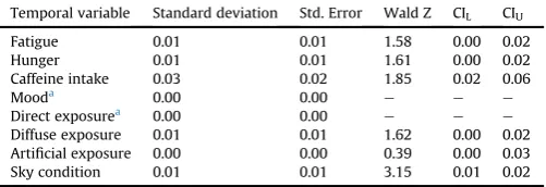
2_{(8)¼180.19,p0.001, r}2_{¼0.51 (moderate), indicating that the}

variances associated with the random effects were significantly different from zero. This provided statistically and practically relevant evidence that inclusion of the random effectsefatigue, hunger, caffeine intake, mood, prior light exposure (direct, diffuse, and artificial), and sky condition e in the mixed-effects model offered a better fit to the data than the fixed-effects MLM, explaining 51% (r2¼0.51) of the variance that was not accounted for in thefixed-effects analysis.

[image:12.595.33.556.84.258.2]

The DGP was again used as the evaluation parameter to assess the variances associated with each temporal variable (random ef-fects). Estimates of the covariance parameters were calculated by the standard deviation (i.e., the square root of the estimated vari-ance), giving an indication of the spread that the random effects can explain within the model.Table 7presents the standard deviation for each temporal variable included in the mixed-effects model, the standard error, the Wald Z test statistic, and the lower (CIL) and

Table 6

Pairwise comparisons between test sessions (fixed-effects MLM).

GSV Shading setting Times of day N(x0, x1) DMNHST Std. Error df CIL CIU Effect size (d)

Just (Im)Perceptible Default shading Morning vs. Midday 49, 37 0.04* 0.01 678.78 0.06 0.01 0.72 Morning vs. Afternoon 49,45 0.13** 0.03 669.21 0.19 0.04 0.74 Midday vs. Afternoon 37, 45 0.08 n.s. 0.03 640.49 0.16 0.00 0.50 User-set shading Morning vs. Midday 72, 72 0.03 n.s. 0.01 675.85 0.05 0.00 0.40 Morning vs. Afternoon 72, 84 0.02 n.s. 0.01 514.32 0.05 0.01 0.18 Midday vs. Afternoon 72, 84 0.01 n.s. 0.01 679.91 0.02 0.03 0.09 Just Noticeable Default shading Morning vs. Midday 47, 61 0.04** 0.01 692.97 0.06 0.02 0.61

Morning vs. Afternoon 47, 44 0.13*** 0.02 706.00 0.19 0.07 1.08 Midday vs. Afternoon 62, 44 0.10*** 0.02 675.00 0.15 0.04 0.73 User-set shading Morning vs. Midday 43, 38 0.03 n.s. 0.01 719.56 0.06 0.00 0.46 Morning vs. Afternoon 43, 26 0.02 n.s. 0.02 654.47 0.07 0.02 0.27 Midday vs. Afternoon 38, 26 0.01 n.s. 0.02 693.69 0.04 0.05 0.14 Just Uncomfortable/Intolerable Default shading Morning vs. Midday 24, 22 0.04 n.s. 0.02 714.30 0.06 0.00 0.80

Morning vs. Afternoon 24, 31 0.14*** 0.03 679.73 0.21 0.06 1.12 Midday vs. Afternoon 22, 31 0.11*** 0.03 661.40 0.19 0.04 0.80 User-set shading Morning vs. Midday 5, 10 0.02 n.s. 0.03 683.06 0.08 0.05 0.44 Morning vs. Afternoon 5, 10 0.00 n.s. 0.03 711.68 0.03 0.03 0.00 Midday vs. Afternoon 10, 10 0.02 n.s. 0.02 704.70 0.01 0.04 0.44

*Weakly significant; ** significant; *** highly significant; n.s. not significant.

d<0.41¼negligible; 0.41d<1.15¼small; 1.15d<2.70¼moderate; d2.70¼large.

Table 7

Estimates of covariance parameters for each random effect (temporal variables).

Temporal variable Standard deviation Std. Error Wald Z CIL CIU

Fatigue 0.01 0.01 1.58 0.00 0.02

Hunger 0.01 0.01 1.61 0.00 0.02

Caffeine intake 0.03 0.02 1.85 0.02 0.06

Mooda _{0.00 0.00 e e e}

Direct exposurea _{0.00 0.00 e e e}

Diffuse exposure 0.01 0.01 1.62 0.00 0.02

Artificial exposure 0.00 0.00 0.39 0.00 0.03

Sky condition 0.01 0.01 3.15 0.01 0.02

[image:12.595.303.554.639.725.2]

upper (CIU) 95% confidence intervals for the standard deviation

associated with each random effect calculated from the multivar-iate Wald test.

The standard deviation (descriptive) and the Wald Z (inferen-tial) statistics both provide a measure of the variance that each temporal variable causes on the DGP. With reference to the stan-dard deviation, the results indicate that caffeine intake caused the highest amount of variance in DGP values (SD¼0.03). Conversely, the Wald Z test statistic associated the sky condition with the highest amount of variance in the DGP (Wald Z¼ 3.15). These conflicting results are likely due to differences in the scaling of the self-reported temporal variables, whereby caffeine intake was measured on a discrete dichotomous scale, while all other variables were measured on a 7-point Likert scale. However, since the Wald Z is a standardised value (comparable across temporal variables), the data suggest that sky condition can explain the highest amount of residual variance in the MLM, which cannot be explained by the

[image:13.595.134.476.505.726.2]

fixed effects alone. That is, the variance in DGP at a between-subject level (expressed by the personal regression slopes for each test subject) is largest when participants were exposed to different sky conditions while reporting their glare sensation for eachfixed ef-fect specified in the MLM.

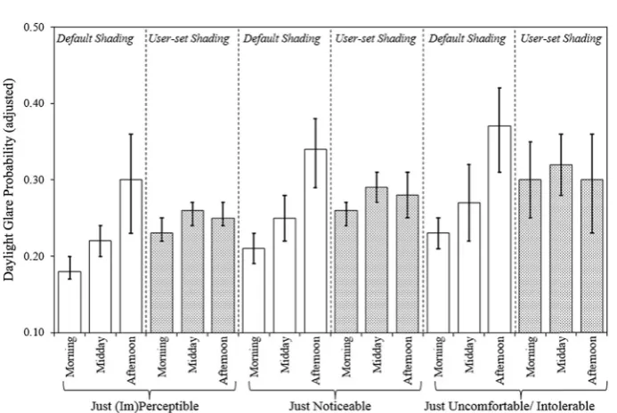
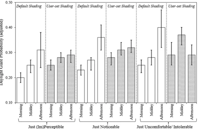
Fig. 11plots the adjusted DGP marginal means (with 95%

con-fidence intervals) controlled for glare source size and position and for the variances associated with the temporal variables included as random effects in the MLM. On the x-axis, thefigure presents the votes of glare sensation organised according to times of day and shading setting. As with thefixed-effects MLM, the GSV criteria of

‘Just Uncomfortable’and‘Just Intolerable’were merged together. The DGP was again calculated at a constant solid angle subtended by the glare source modified by the position index (

U

¼0.27).

Under the default shading setting, consistent withFig. 10, the displays show a consistent trend for central tendencies to corre-spond to increasing levels of DGP for each GSV as the day pro-gresses, hence confirming the outcomes of thefixed-effects MLM and supporting the hypothesis of a temporal effect on glare response from daylight when venetian blinds were set at their cut-off position.

Under the user-set shading, contrary to thefixed-effects anal-ysis, in the mixed-effects MLM an equivalent trend can also be

observed for the GSV criteria of Just (Im)Perceptible and Just Noticeable, with central tendencies corresponding to higher levels of DGP at later test sessions. This trend, however, does not appear to be as strong as under the default shading setting, and it is not evident for the combined GSV criterion of Just Uncomfortable/ Intolerable.

Table 8 shows the inferential data from the univariate tests (mixed-effects MLM), providing the shading setting, the GSV criteria, the degrees of freedom (df), the test statistic (F), and the statistical significance (p-value).

Under both shading settings, the results returned statistically significant differences in DGP values.

For each GSV criterion,Table 9presents the results of the con-trasts made to isolate the main effects between variables, providing the shading setting, the number of glare assessments (N) reported by test subjects (x0 and x1 corresponding to the test sessions

considered in the pairwise comparisons), the difference between the estimated DGP marginal means (

D

M) and its associated two-tailed statistical significance (NHST, p-value with Bonferroni correction), the standard error, the degrees of freedom (df), the lower (CIL) and upper (CIU) 95% confidence intervals for the

dif-ference between marginal means, and the effect size (d).

Under the default shading setting, as for thefixed-effects MLM, the mean differences (

D

M) and effect sizes (d) were consistently negative. The pairwise comparisons detected statistically signifi -cant and practically relevant differences in all but one case. The mixed-effects inferential tests, thus, con_firmed evidence of a tem-poral effect on glare response when blinds were set at their cut-off position.

Under the user-set shading, descriptive statistics (

D

M) and ef-fect sizes showed consistent negative signs for the ‘Just (Im) Perceptible’and‘Just Noticeable’GSV criteria. Statistically signifi -cant and practically relevant differences were detected in 5 cases. Therefore, when blinds were adjusted by test subjects, after con-trolling for the influence of temporal variables across the fi xed-effects (i.e., time of day, shading setting, and GSV), the mixed-effects MLM also provided some evidence of an effect of time of day on glare sensation from daylight, with the exception of the‘Just Uncomfortable/Intolerable’criterion for which results did not allow the de_finition of a prevailing tendency.

3.3. Magnitude of temporal influences

With respect to thefindings from the initialfixed-effects MLM and from previous laboratory studies[11,12,14], the results of the mixed model analysis demonstrated that, when controlling for the temporal variables (random effects), indications of a direct infl u-ence of time of day on glare response from daylight could be detected under both shading settings. In addition, the outcomes of the inferential tests signalled that the temporal influence amplifies as the day progresses, thereby suggesting that test subjects became increasingly tolerant to the glare source at later times of day.

It is worth considering that thefixed-effects MLM provided no evidence of an effect of time of day on subjective glare response when participants were given the possibility to control the vene-tian blinds (Table 6). Conversely, the influences of the random ef-fects within the mixed model suggested that the variances associated with the temporal variables partially confound the effect of time of day on reported glare sensation. That is, once the vari-ances of temporal variables were controlledehence, increasing the sensitivity of the inferential tests[41]ean effect of time of day on glare response could be detected also under the user-set shading setting. However, since the magnitude of the temporal influences (effect size) was generally smaller under the user-set shading (Table 9), it is plausible thatewhen blinds were adjusted by test subjectsethe presence of other uncontrolled variables or condi-tions might have further masked or confounded the influences of the temporal effects on glare perception.

Interestingly, when considering the default shading setting, the effect sizes calculated from the pairwise comparisons in thefi xed-effects (Table 6) and mixed-effects (Table 9) MLM models do not differ substantially. This leads to the hypothesis that the temporal

variables may have more influence on glare sensation once the participants regulated the venetian blinds to their own visual preference.

4. Discussion

The results of an experiment conducted in a test room with direct access to daylight and to an external view have provided evidence of a statistically signi_ficant and practically relevant effect of time of day on glare response. Supporting the conclusions of an earlier artificial lighting laboratory study [11], the influences detected showed that the time interval between test sessions had a direct relationship with increases in tolerance to discomfort from daylight glare. In fact, when providing their judgement at later times of day (under a randomised sequence of test sessions), sub-jects gave the same assessment of glare sensation (i.e., GSV) to conditions characterised by higher probability of glare occurrence. The effect of time of day on glare response was particularly evident when venetian blinds were set at a cut-off position ensuring predominantly diffuse daylight conditions. Conversely, when blinds were adjusted by the participants, evidence of tem-poral in_fluences on glare sensation was not detected by an initial

fixed-effects multilevel model (MLM) analysis.

[image:14.595.32.553.87.155.2]

Since previous laboratory studies had revealed a substantive influence of temporal variables (e.g., fatigue, food ingestion, caffeine intake, prior light exposure, sky condition) on glare response[12], a mixed-effects MLMeconsidering factors that were experimentally manipulated (fixed effects) and variables that changed over time (random effects)e was fitted to analyse the data. The mixed-effects MLM supported thefindings of thefi xed-effects analysis under the default shading setting, and also

Table 8

Univariate tests (mixed-effects MLM).

Shading GSV Numerator df Denominator df F p-value

Default shading Just (Im)Perceptible 2 483.19 6.90 0.00***

Just Noticeable 2 505.79 21.21 0.00***

Just Uncomfortable/Intolerable 2 575.36 10.90 0.00***

User-set shading Just (Im)Perceptible 2 358.37 9.61 0.00***

Just Noticeable 2 581.18 4.43 0.01**

Just Uncomfortable/Intolerable 2 551.30 7.89 0.00***

*Weakly significant; ** significant; *** highly significant; n.s. not significant.

Table 9

Pairwise comparisons between test sessions (mixed-effects MLM).

GSV Shading setting Times of day N(x0, x1) DMNHST Std. Error df CIL CIU Effect size (d)

Just (Im)Perceptible Default shading Morning vs. Midday 49, 37 0.05** 0.01 448.67 0.07 0.02 0.77 Morning vs. Afternoon 37, 45 0.06 n.s. 0.04 517.88 0.14 0.03 0.31 Midday vs. Afternoon 49, 45 0.11* 0.04 511.83 0.17 0.01 0.56 User-set shading Morning vs. Midday 72, 72 0.03*** 0.01 393.96 0.05 0.01 0.38 Morning vs. Afternoon 72, 84 0.01 n.s. 0.01 331.90 0.03 0.02 0.12 Midday vs. Afternoon 72, 84 0.04*** 0.01 423.84 0.06 0.01 0.47 Just Noticeable Default shading Morning vs. Midday 47, 61 0.04*** 0.01 439.42 0.06 0.02 0.53 Morning vs. Afternoon 62, 44 0.09*** 0.03 582.54 0.16 0.04 0.59 Midday vs. Afternoon 47, 44 0.13*** 0.03 559.85 0.20 0.08 0.87 User-set shading Morning vs. Midday 43, 38 0.03* 0.01 491.42 0.06 0.01 0.46 Morning vs. Afternoon 38, 26 0.01 n.s 0.02 626.91 0.04 0.03 0.12 Midday vs. Afternoon 43, 26 0.04 n.s. 0.02 613.83 0.07 0.00 0.47 Just Uncomfortable/Intolerable Default shading Morning vs. Midday 24, 22 0.03* 0.02 584.25 0.07 0.01 0.41 Morning vs. Afternoon 22, 31 0.12** 0.04 576.32 0.20 0.03 0.71 Midday vs. Afternoon 24, 31 0.15*** 0.04 558.94 0.24 0.07 0.94 User-set shading Morning vs. Midday 5, 10 0.08** 0.02 557.35 0.13 0.02 1.57 Morning vs. Afternoon 10, 10 0.08*** 0.02 570.44 0.03 0.13 1.33 Midday vs. Afternoon 5, 10 0.00 n.s. 0.02 573.90 0.06 0.06 0.00

*Weakly significant; ** significant; *** highly significant; n.s. not significant.

[image:14.595.33.557.205.381.2]