Bayesian Processing of Big Data using Log Homotopy Based Particle Flow Filters

This is a repository copy of

Bayesian Processing of Big Data using Log Homotopy Based

Particle Flow Filters

.

White Rose Research Online URL for this paper:

http://eprints.whiterose.ac.uk/121517/

Version: Accepted Version

Proceedings Paper:

Khan, A.M., De Freitas, A., Mihaylova, L.S. orcid.org/0000-0001-5856-2223 et al. (2 more

authors) (2017) Bayesian Processing of Big Data using Log Homotopy Based Particle

Flow Filters. In: 2017 Sensor Data Fusion: Trends, Solutions, Applications (SDF). The 11th

Symposium Sensor Data Fusion: Trends, Solutions, and Applications, 10-12 Oct 2017,

Bonn, Germany. IEEE . ISBN 978-1-5386-3103-4

https://doi.org/10.1109/SDF.2017.8126349

[email protected] https://eprints.whiterose.ac.uk/ Reuse

Items deposited in White Rose Research Online are protected by copyright, with all rights reserved unless indicated otherwise. They may be downloaded and/or printed for private study, or other acts as permitted by national copyright laws. The publisher or other rights holders may allow further reproduction and re-use of the full text version. This is indicated by the licence information on the White Rose Research Online record for the item.

Takedown

If you consider content in White Rose Research Online to be in breach of UK law, please notify us by

Bayesian Processing of Big Data using Log

Homotopy Based Particle Flow Filters

Muhammad Altamash Khan

, Allan De Freitas

, Lyudmila Mihaylova

, Martin Ulmke

and Wolfgang Koch

Email:_{altamash.khan,martin.ulmke,wolfgang.koch_}@fkie.fraunhofer.de

†_{Department of Automatic Control and Systems Engineering, University of Sheffield, United Kingdom}

Email: _{a.defreitas,L.S.Mihaylova_}@sheffield.ac.uk

Abstract—Bayesian recursive estimation using large volumes

of data is a challenging research topic. The problem becomes particularly complex for high dimensional non-linear state spaces. Markov chain Monte Carlo (MCMC) based methods have been successfully used to solve such problems. The main issue when employing MCMC is the evaluation of the likelihood function at every iteration, which can become prohibitively expensive to compute. Alternative methods are therefore sought after to over-come this difficulty. One such method is the adaptive sequential MCMC (ASMCMC), where the use of the confidence sampling is proposed as a method to reduce the computational cost. The main idea is to make use of the concentration inequalities to sub-sample the measurements for which the likelihood terms are evaluated. However, ASMCMC methods require appropriate proposal distri-butions. In this work, we propose a novel ASMCMC framework in which the log-homotopy based particle flow filter form an adaptive proposal. We show the performance can be significantly enhanced by our proposed algorithm, while still maintaining a comparatively low processing overhead.

Keywords—Particle flow filters , Log-homotopy , DHF , big data, SMCMC, Confidence sampling, Multiple target tracking.

I. INTRODUCTION

The presence of a large number of measurements can be considered as a ”big data” problem. It faces serious compu-tational challenges, in particular for numerical methods like sequential Monte Carlo (SMC) and sequential Markov chain Monte Carlo (SMCMC). The problem can be pinpointed to the computation of the likelihood term, or its derivatives which become the bottle neck. Dimensionality reduction may be employed, for example through data clustering, but it is unclear whether the samples generated thereof still belong to the true posterior distribution. An interesting solution has been provided in [1] based on an earlier work done in [2], where probabilistic subsampling also termed as the confidence sam-pling has been employed to reduce the number of likelihood evaluations in the context of SMCMC. A major benefit of this approach is that it comes with a theoretical guarantee regarding the generated samples, i.e. the sampled distribution lies within a user specified tolerance of the true posterior distribution. On the other hand, the use of a better suited proposal distribution is one of the key requirements for the algorithm. While for some problems the selection of the proposal could be straightforward e.g. for moderately nonlinear or Gaussian models, for others the choice may not be that obvious.

In this paper, we present a novel approach for the Bayesian processing of the big data by combining the log-homotopy

based particle flow (DHF) together with the SMCMC. We propose an initial measurement clustering, after which the log homotopy flow is applied. The samples after the flow are as-sumed to be approximately in the vicinity of their true posterior locations, though not exactly there. Hence, they can form an excellent proposal to be used within the subsequent confidence sampling driven MCMC procedure. The main purpose of the last step is to profit from the convergence guarantee that comes associated with later procedure. In this way, we essentially bring the strength of both methods under one banner.

The paper is organized as follows. The problem formula-tion and the possible approaches for big data processing via SMCMC are highlighted in section II. This is followed by section III, where the probabilistic subsampling i.e. confidence sampling methodology is discussed in the detail. Potential issues with the choice of proposal distribution for SMCMC are mentioned in section IV. The use of DHF together with the data clustering to form a better proposal is also advocated in the same section. In section V, we describe our newly devised DHF based confidence sampling driven SMCMC algorithm. Mathematical models and simulation setup for the test scenario used in evaluation of the new scheme are presented in section VI. Performance evaluation of our scheme is detailed in section VII, which is followed by the conclusion in section VIII.

II. BIG DATA PROCESSING USINGMCMC

Let xk ∈Rd denote the state vector and zk ∈Rm denote the measurement vector at time k. Furthermore, let Zk denote the set of measurements up to time k including zk, such that,

Zk = {z1, z2 , ... , zk }. Then according to the Chapman-Kolmogorov equation and the Bayes theorem, the prior den-sity p(xk+1|Zk) and the posterior density p(xk+1|Zk+1) are

recursively defined as,

p(xk+1|Zk) =

Z

p(xk+1|xk)p(xk|Zk)dxk (1)

p(xk+1|Zk+1) =

p(zk+1|xk+1)p(xk+1|Zk) p(zk+1|Zk)

(2)

In the case that all measurements are independent, the likeli-hood can be written as,

p(zk+1|xk+1) =

Mk

Y

i=1

where Mk is the number of measurements present at time k. For big data, Mk >>1. An exact closed form solution of (1) and (2) is generally not available for nonlinear systems.

Markov chain Monte Carlo methods were invented to simulate the dynamics of gaseous systems in equilibrium [3]. Sequential MCMC started to appear in the target tracking literature as an alternative to the importance sampling for sampling higher dimensional spaces. SMCMC, as used in the target tracking application [4],[5] and [6],differs from SMC in that they do not sample from the posterior distribution directly. Instead, at each time instance k, a stationary, reversible jump, Markov chain is constructed through a Markov transition kernel q(xy_k+1|xx_k+1). The kernel is also referred to as the proposal. The chain is started at an arbitrary location and is continuously lengthened by appending samples. The chain is assumed to have the posterior distributionp(xk+1|Zk+1)as its

stationary distribution. Every new sample generated through the proposal distribution is either accepted or rejected, based on the Metropolis Hastings procedure (MH).

Big data describes the situation where a large number of observations / measurements are available to be processed at any time instant. This can occur in several situations. In the most typical scenario, big data could arise in the tracking of a single or multiple target(s) using the measurements gathered through a multitude of sensors. Examples are bearing only estimation in the presence of clutter [7], and in the presence of position biases and offsets [8]. Alternatively, big data can occur when the tracked target(s) can no longer be modelled as point source object(s) due to the enhanced sensor resolution, for example in the case of extended object tracking [9]. The presence of big data can render the employment of traditional state estimation methods like EKF/UKF inadequate, while other methods like SMC and SMCMC could simply be computationally too expensive.

MCMC processing for big data has been a subject of continuing research. The proposed methods can largely be categorized into two main classes. The first class of methods uses the so called divide and conquer approach, where mea-surements are divided into non-overlapping batches or blocks to be processed by individual processers. Divide and conquer methods, though quite simple in terms of tractability and implementation, rely on the underlying Gaussian assumption for the data. Their performance degrades when the assumption of local Gaussianity is violated. The other class of methods uses the idea of subsampling or decimation of the measurement set, such that the MCMC is only applied to a subset of the whole data.

III. CONFIDENCE SAMPLER: PROBABILISTIC SUBSAMPLING WITHINMCMCFRAMEWORK

An interesting approach has been proposed in [10], where the probabilistic subsampling of the data has been introduced. It relies on the use of the so called concentration inequal-ities, which provide a theoretical bound on the maximum absolute deviation of the average likelihood ratio. The method automatically selects a subset of the measurement data based on the evaluation of a stopping criterion. The MH accept-reject decision is based on a user defined probability 1-δ. The resulting Markov chain is uniformly ergodic provided that the

original chain also has the said property. Most importantly, the algorithm provides a theoretical guarantee that the sam-pled density is with the _O(δ) of the true posterior density

p(xk+1|Zk+1). The disadvantage of the approach is that the

evaluation of the stopping criterion is based on a measure of the range of the log-likelihood ratio set, which except for few simple cases requires likelihood calculation for the whole data set. Concentration inequalities are the worst case assurances but they carry with them an additional processing cost. Since the method utilizes a confidence bound, it is termed as the confidence sampler. Next, we briefly mention the highlights of the confidence sampling procedure.

We begin with the formulation of the Metropolis Hastings step for proposing a new sample in a MCMC chain,

u < p(x

∗

k+1|Zk+1)q(x_km₊₁−1|x∗k+1)

p(xm_k+1|Zk+1)q(x∗_k+1|xm_k+1−1)

(4)

whereu_{∈ U}[0,1],q(._|.) is the proposal distribution whilem

is the chain iteration index. Now assuming that the likelihood can be decomposed into individual terms i.e. assuming inde-pendence of the measurements (3), we can re-write as (2),

u < p(x

∗

k+1|Zk)q(xmk+1|x∗k+1)

p(xm_k+1|Zk)q(x∗k+1|x

m−1

k+1 )

M

Y

i=1

p(zi_k+1|x∗_k+1)

p(zi_k+1|xm_k+1) (5)

Further manipulation of the equation leads to,

ψ(xm_k+1,x∗_k+1)<ΛM(xmk+1,x∗k+1) (6)

where,

ψ(xm_k+1,x∗_k+1) = 1

M log

up(x

∗

k+1|Zk)q(xmk+1|x∗k+1)

p(xm_k+1|Zk)q(x∗k+1|xmk+1)

ΛM(xmk+1,x∗k+1) =

1

M M

X

i=1

log

"

p(zi_k+1|x∗_k+1)

p(zi_k+1|xm_k+1)

#

The left side of the inequality is independent of the data, while the right hand side exclusively depends on the measurements. We define the average log-likelihood ratio using the full data set asΛM. When using a subset of measurements of sizeNm, the average log-likelihood ratio can be defined as,

ΛNm =

1

Nm M

X

i=1

log

"

p(zi_k+1|x∗_k+1)

p(zi_k+1|xm_k+1−1)

#

(7)

Concentration inequalities can be used to define to obtain a bound on the ΛNm.

P(|ΛM(xmk+1,x∗k+1)−ΛNm(x m

k+1,x∗k+1)| ≤cNm)≥1−δNm (8) whereδNm is a used-defined threshold (probability) and cNm is dependent on the particular form of inequality used. In this work, we use Bernstein’s inequality, as suggested in [2], which results in,

cNm =

s

2VNmlog(3×δ −1

Nm)

Nm +

3Rlog(3×δ_N−1

m)

Nm

(9)

note that the accept-reject decision is based on evaluation of (6). The average log-likelihood ratio based on the whole data set is not of our interest, instead, we would like to base our decision onΛNm(x

m

k+1,x∗k+1). It results in a stopping criterion

|ΛNm_(xm−1

k+1,x∗k+1)−ψ(xkm+1,x∗k+1)|> cNm. This, when seen in the light of the concentration inequality, can be interpreted as taking the right decision with probability at least 1-δNm, if the stopping criterion is met.

We start with the user-defined parameter δs ∈ (0,1). The algorithm begins with an empty set for the subsam-pled measurements _Zk. At each iteration, measurements are added to the subset and the stopping criterion is checked. The data aggregation stops as soon as _|ΛNm_(xm−1

k+1,x∗k+1)−

ψ(xm_k+1,x∗_k+1)_| > cNm holds true, or all measurements have been added to the set_Zk+1, in which case the accept-reject

de-cision is based on the evaluation of the full data set. Forps>1, we set δNm =

ps−1 psNm,kps δs

which leads to ΣNm,k>1δNm ≤δs. The event,

E = \

Nm,k≥1

{|ΛM(xm_k+1−1,x∗_k+1)₋ΛNm_(xm−1 k+1,x

∗

k+1)| ≤cNm} (10) therefore holds with the probability of at least 1₋δNm. The range in (9) requires the evaluation of log-likelihood ratios for the whole data set. While for some problems the range can be computed straightforwardly e.g. in the case of a Gaussian likelihood, this is generally not the case. Thus any potential gain achieved by subsampling the data is lost.

To alleviate the problem of the still high processing cost, an approximate method is presented in [2] which makes use of the so-called proxies. Proxies are supposed to be cheap to evaluate, but at the same time should approximate the actual likelihood term sufficiently well. The resulting algorithm yields empirical gains, but still keeps the guarantees of the original scheme. Additionally, proxy terms act as control variate, therefore reducing the variance of the estimates.

The introduction of the proxy term leads to the modification of the termΛNm,

ΛNm =

1

Nm M

X

i=1 (

log

"

p(zi_k+1|x∗_k+1)

p(zi_k+1|xm_k+1−1)

#

−P_i(xm−1

k+1,x∗k+1) )

(11)

Amongst several choices available for the proxy terms, the simplest is provided by the first order Taylor series expansion [1],

P_i(xm_k+1−1,x∗_k+1) = (_∇ℓ )T_x+

k

.(x∗_k+1−xm_k+1−1) (12) where _∇ℓ is the gradient of the log-likelihood and the linearization is carried out about some point x+_k+1. This leads to the following form of the range,

RB_k+1= 2 max

1≤i≤M{|Bk+1(x m−1

k+1)−Bk(x

∗

k+1)|} (13)

where Bk+1(.) is the Hessian matrix of the log-likelihood.

Also, the maximum is taken of the absolute values of the difference matrix entries. The main advantage of using the Taylor series based proxy is the ease in computation of the proxy terms and the range measure R. The full confidence sampling algorithm using proxies is described in the Algorithm 1.

Algorithm 1 Confidence sampler with proxy

1: procedure CONFSAMPLER

2: Nm,k+1 = 0 ⊲ Number of subsampled measurements

3: ΛNm = 0 ⊲ Subsampled log-likelihood 4: Z_k∗₊₁=∅ ⊲Set of subsampled measurements

5: lN = 1 ⊲Batch size

6: i = 0 ⊲ Loop counter

7: FLAG = UP ⊲ Flag variable

8: ComputeRB_k+1 according to (13) ⊲Range 9: while FLAG == UP do

10: i = i + 1 11: {zNm,k+1+1,∗

k+1 ,· · · ,z

b,∗

k+1} ∼w/repl.Zk+1\zk+1

12: Z_k∗₊₁=Z_k∗₊₁∪ {zNm,k+1+1,∗ k ,· · ·,z

b,∗ k+1}

13: Ω= ΣlN

j=Nm,k+1+1

logp(z j,∗

k+1|x∗k+1)

p(zj,∗

k+1|xmk+1)

−P_i(xm k+1,x∗k+1)

14: ΛNm= l1N Nm,k+1×ΛNm+Ω

15: Nm,k+1=lN

16: δNm =

ps−1 psipsδs

17: Compute c according to (9) 18: lN =γmcmcNm,k+1∧Mk+1

19: if _|ΛNm+

1

Mk+1 Mk+1

P

i=1

P_i(xm_k+1,x_k∗₊₁)₋ψ(.)_{| ≥}c

orNm,k==Mk then

20: FLAG = DOWN

21: end if

22: end while

23: return ΛNm,{Pi(x m

k+1,x∗k+1)}

Mk+1 i=1

24: end procedure

IV. ABETTER PROPOSAL DISTRIBUTION FOR THEMH STEP

As alluded to in the introduction, the log-homotopy based particle flow can be used to form a better proposal. This is ow-ing to the fact that the flow incrementally moves the particles towards their posterior locations by gradually incorporating the measurements. This helps to solve the issue of degeneracy in a standard estimation problem. DHF, if carefully implemented, can also be computationally cheaper than a standard particle filter [11]. Hence, it comes naturally to use the particles out of the DHF to form the proposal distribution for the subsequent MCMC step. Below we describe some basics of the homotopy based particle flow and its implementation methodology.

A. Log homotopy based particle flow

The whole procedure is shown as a pseudo-code in the Algorithm 2. Here _{ˆxi_k+1}Np

i=1 and {¯xik+1}

Np

i=1 are the set of

prior and posterior particles, respectively. We plan to use the DHF based approximation of the posterior density as the proposal distribution in the confidence sampler based SMCMC i.e. q(xk+1|.)≈pˆDHF(xk+1|Zk+1). We follow the

factor here. As it can be noted [11], the nonzero diffusion constrained flow equation requires the Hessian of the log-likelihood function. A direct application of the DHF in a big data scenario, therefore, can become prohibitively expensive. The question becomes, how to use the DHF while maintaining a reasonably low processing cost. One answer to this problem lies in the decimation of the measurement set.

Algorithm 2 Log homotopy flow based measurement update

1: procedure LOGHOMOTOPYFLOWUPDATE 2: Pˆk+1 = SHRINKAGEESTIMATOR(ˆxi_k+1) 3: for i = 1 :Np do

4: y₀ = ˆxi_k+1

5: for j = 1 :Nλ do

6: Hλ = GETHESSIAN(logh(zk|yj−1) )

7: hλ = GETGRADIENT(logh(zk|yj−1))

8: m(y_j)= -hPˆ−_k1+λjHλ

i−1

hT_λ

9: y_j = y_j−1 + m(y_j)∆λj

10: end for

11: ¯xi_k+1 = y_Nλ 12: end for

13: Evaluate the posterior mean µµµ¯¯¯k+1 and covariance

matrixP¯k+1

14: REDRAWPARTICLES(_{¯xi_k+1}Np i=1)

15: return _{xi_k+1}Np

i=1,µµµ¯¯¯k+1 ,P¯k+1

16: end procedure

The second question relates with the finding of an an-alytical approximation for pˆDHF(xk|Zk), for its subsequent sampling and evaluation in the ASMCMC procedure.

B. Data reduction

We tackle the issue of dimensionality reduction through clustering. Clustering turns out to be quite effective means of dimensionality reduction. We use K-medoids clustering, with the partitioning done around medoids. A medoid is a point within a cluster whose average dissimilarity to all other points in the cluster is minimal, i.e. it is a most centrally located point in the cluster. K-medoids clustering is said to be more robust to noise and outliers as compared to K-means clustering because it minimizes a sum of pairwise dissimilarities instead of a sum of squared Euclidean distances.

C. Proposal density representation

As discussed before, the output of the DHF are the approx-imated posterior samples, represented through the Dirac-delta approximation. For it to be used as a proposal density within a MCMC step, it has to be further approximated by some closed form probability density expression. As described in [11], the redrawing step in the Algorithm 2 (step 14) returns the approximated density either as a single multivariate Gaussian (MVG) or as a Gaussian mixture model (GMM). In the current work, we use a MVG approximated form for the proposal density.

V. SEQUENTIALMCMCWITHDHFBASED PROPOSAL FOR BIG DATA PROCESSING

In [1], MCMC is used together with the confidence sampler to estimate a high-dimensional non-Gaussian state. The overall procedure is termed as Adaptive Sequential Markov chain Monte Carlo (ASMCMC). The algorithm is based on two main steps: an initial joint drawing of the xk,xk−1 with the target

density,

p(xk,xk−1|Zk−1)∝p(xk|xk−1)p(xk−1|Zk−1) (14)

and a secondary refinement step redrawing both of these variables individually. ASMCMC has three sub stages, each of which uses an MH step, with the first and the third employing the confidence sampling since the likelihood evaluations are involved.

Algorithm 3 Adaptive SMCMC with particle flow based

proposal

1: procedure SMCMCWITHPARTICLEFLOW 2: Initialize the particle_{¯xi0}

Np i=1

3: for k = 1 : kmax do

4: zc_k = CLUSTERMEASUREMENTS(zk )

5: zc_kˆ = LIKELIHOODBASEDCOMPRESSION(zc_k ) 6: {ˆxi_k}Np

i=1 = PRIORSAMPLING({¯xik−1}

Np i=1)

7: {¯xi_k}Np

i=1 = LOGHOMOTOPYFLOWUPDATE

8: q(x∗_k|xm_k )= GETPROPOSALDENSITY(_{xi_k}Np i=1)

9: Markov chain Monte Carlo 10: Initialize the Markov chain: x0_k 11: for m = 1 :Nc+Nb do

12: if m = 1_∨Nb then

13: UPDATEPROXYPARAMETERS

14: end if

15: x∗_k∼q(x∗_k|xm_k )

16: ψ(xm_k,x∗_k) = _M1 loghup(x∗k|Z k−1_)q(xm

k|x∗k) p(xm

k|Zk−

1_)q(x∗

k|xmk)

i

17:

h

ΛNm,{Pi(x m k ,x∗k)}

Mk i=1 i

=CONFSAMPLER

18: ̺Mk =ΛNm−ψ(x m

k ,x∗k)+ M1k n

P

i=1

P_i(xm_k,x∗_k)

19: if ̺Mk>0 then

20: xm_k =x∗_k

21: else

22: xm_k =xm_k−1

23: end if

24: end for

25: p¯(xk|Zk)= _N1_p Np

P

i=1

δ(xk−¯xik)

26: end for

27: end procedure

Transitional density is used to form proposals distributions in the MH steps. ASMCMC has been shown to sample posterior density reasonably well, with lesser execution time when compared to the plain MCMC while still maintaining a reasonable performance. The confidence sampling is the key in reducing the computational burden.

been described in the earlier sections, the task at hand is to embed all of them within a unified framework. We call the scheme Adaptive SMCMC with particle flow based proposal or ASMCMC-DHF. It is described in the Algorithm 3. The optional secondary level data compression method is based on choosing the most likely samples from the set of the previously clustered measurements.

VI. MODEL& SIMULATION SETUP

In order to test the performance of our algorithm, we consider a multi-target tracking scenario in the presence of clutter, similar to the one used in [1]. However, as a distinction, we use a nonlinear measurement model. Observations are generated by a sensor located at the origin and consist of range and bearing of the targets. The state vector for the target i at time instant k is x_k(i)=(x_k(i), y_k(i),x˙_k(i),y˙(_ki)), wherex_k(i)andy(_ki)

represent the position whilex˙(_ki)andy˙_k(i)representing velocity components along the x and y-axis respectively. We assume a discrete white noise acceleration model (DWNA). Since we are considering a big data scenario, multiple measurements per target are generated. The number of measurements per targets are considered to be Poisson distributed with intensity λx. In addition to the target returns, there are clutter measurements whose number at any time instance is also Poisson distributed with intensity λc. Furthermore, target-data association is not assumed to be known, but we do not use any data association algorithm. This is justified as the main purpose of this work is to test the efficacy of the use of DHF together with ASMCMC. The total number of measurements received at the time in-stance k is given byµk =NTMkx+Mkc, whereMkxrepresents the number of measurements per target (considered same for all targets) andMc

k the number of clutter measurements. The joint likelihood can then be expressed as,

l(xk) = e−µk

Mk! Mk

Y

i=1 

λcpc(z

i k) +λx

NT

X

j=1

px(zik|xk,j)



 (15)

The measurement vector for the target i is given by z(_ki) = (r(_ki), θ_k(i)), where r(_ki) is the range to the target while θ(_ki)

is the target bearing and with the sub-likelihood getting the form px(zi_k|xk,j) = pi,jx = N(zik|h(xk,j),Rk), with

h(xk,j) =

h√

xk,j+yk,j,tan−1

_y

k,j xk,j

iT

and Rk being the measurement covariance matrix. The clutter measurements are independent of the target measurements and are thought to be uniformly distributed within the surveillance area i.e.

pc(zik) =Ux(µ(zk,r, zk,θ))Uy(µ(zk,r, zk,θ)).

Parameter Value Parameter Value Parameter Value

Np 100 Nmcmc 400 Nburn Nmcmc/4

γmcmc 1.5 δs 0.1 ps 2

Ts 1 λx 50/500 λc 200/2000

σ2

x 0.5 σ

2

r 10 σ

2

θ 0.01

Ameas 400×400 Tsim 50 Kclust 30 Table I: Parameters

We consider tracking of two targets (NT=2), under two separate conditions: a moderately big data scenario withλx=50 andλc=200, and an extremely big data scenario withλx= 500 andλc= 2000. In the subsequent analysis, we will refer to the former case as the BD1 (big data 1), while the later as BD2 (big data 2). We use K-medoids clustering with 30 medoids for the initial clustering of the measurement data. The two

targets start at position (-50 , -50) and (30 , 30), whereas initial velocities for the two targets are given by (-0.1 , -0.1) and (0.1 , 0.5) respectively. We consider 100 particles for DHF

Np = 100 and 30 geometrically spaced pseudo-time points for solving log-homotopy flow ODE. We use root average mean square error (RAMSE) as the performance metric. We simulated each scenario a total of fifty times (Nsim = 50), with each simulation running for a total of 50 time steps. The standard parameter setting are shown in Table I.

VII. RESULTS

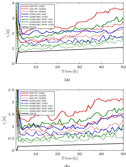
We compare the performance of our proposed ASMCMC-DHF scheme against other methods. In the current analysis,we have used two such methods: the sampling importance re-sampling particle filter (SIR-PF) with 1000, 10000 and 25000 particles, and the ASMCMC method as described in [1] with 500 and 1250 MCMC chain lengths. The effort is made to make the comparison fair, in the sense of similar execution times for all procedures. Simulation were run on a server using MATLAB version 7.9 with 2x Intel Xeon E5530 2.40 GHz processors and with 12GB of RAM. In figures 1 a&b, we plot the RAMSE for all schemes under comparison together with the Cr¨amer-Rao Lower Bound (CRLB),

10 20 30 40 50

Time[k] 0

1 2 3 4

ǫr

[m

]

SIR-PF-1000 SIR-PF-10000 SIR-PF-25000 ASMCMC-500 ASMCMC-1250 ASMCMC-DHF-125 ASMCMC-DHF-500 ASMCMC-DHF-1250 CRLB

(a)

10 20 30 40 50

Time[k] 0

0.5 1 1.5 2 2.5

ǫr

[m

]

SIR-PF-1000 SIR-PF-10000 SIR-PF-25000 ASMCMC-500 ASMCMC-1250 ASMCMC-DHF-125 ASMCMC-DHF-500 ASMCMC-DHF-1250 CRLB

(b)

Figure 1: Comparison of ASMCMC-DHF with other schemes for (a) λx= 50,λc=200, (b)λx = 500,λc=2000

Method RAMSE[m] Acceptance rate Compression ratio Processing time[s]

SIR-PF-1000 2.42/1.57 - - 4.31/33.86

SIR-PF-10000 1.8/1.05 - - 57.27/324.52

SIR-PF-25000 1.73/0.82 - - 144.02/676.21

ASMCMC-500 2.10/0.98 0.27/0.20 1.01/2.01 128.07/486.28 ASMCMC-1250 1.52/0.70 0.25/0.18 1.05/2.57 372.48/1249.43 ASMCMC-DHF-125 2.19/1.18 0.27/0.22 1.97/2.42 42.92/74.28 ASMCMC-DHF-500 1.24/0.54 0.24/0.21 2.52/2.69 77.14/179.37 ASMCMC-DHF-1250 1.17/0.49 0.23/0.21 2.67/2.77 125.11/411.47

Table II: Median RAMSE, Acceptance rate and Compression ratio for different filtering schemes under BD1/BD2

potential improvements to be gained by further increasing the number of particles. The error for BD2, naturally, is lesser than for BD1. Next, we discuss the results for ASMCMC. Again, we note a significant drop in the RAMSE by the increase of MCMC chain length from 500 to 1250. ASMCMC-500 seems to have performance similar to the SIR-PF-10000, while with increasing the chain length to 1250 makes performance similar to that of the latter with 25000 particles. The difference is quite noticeable in the RAMSE for the two schemes in the case of BD1. Although, ASMCMC based schemes exhibit quite decent median acceptance rate they have rather insignificant compres-sion ratio. This means that to achieve better performance, the whole data needs to be exhausted therefore defeating the very purpose of using the confidence sampling. Next, we discuss the results for ASMCMC-DHF. It is to be noted that 20% of the initial samples of the chain are considered to be from the burn-in phase and subsequently discarded. For a chain length of 125, we note that the error is quite high, only slightly below the SIR-PF-1000. This illustrates that although the clustering based DHF proposal is better than a simple particle filter, with a too short MCMC chain could be detrimental to the overall performance. We note drastic reduction in the error with the use of a moderate chain length of 500. Finally, we discuss the processing time for a single update step (both time and measurement) for all procedures. SIR-PF-1000 is the fastest of all methods, while ASMCMC-1250 being the slowest. The latter is because of the double use of the confidence sampling. Furthermore, we note that the SIR-PF-25000 and the ASMCMC-DHF-1250 have execution times comparable to that of the ASMCMC-500, although the latter has higher error. ASMCMC-1250, can be seen as the most optimal method offering a right trade-off between the estimation accuracy and the execution speed.

In the retrospect, it can be seen that the choice of the proposal density quite significantly affects the performance. A better choice for the proposal, e.g. using DHF particles not only decreases the error, it also takes lesser time for sampling the posterior density in the MCMC step.

VIII. CONCLUSION

A large number of measurements provides a high informa-tion content, leading to an increased estimainforma-tion accuracy. How-ever, this comes with enhanced computational requirements, hence limiting the use of many standard estimation methods such as MCMC. In this work, inspired by ideas from [1], we propose con?dence sampling based MCMC within the log-homotopy based particle ?ow ?lters. The log-log-homotopy filter is used to construct adaptive proposals. We have termed our newly proposed method as the Adaptive SMCMC with particle flow based proposal or ASMCMC-DHF. It has been shown that our method not only outperforms the well established methods like the particle filter, but also performs better than its parent algorithm, ASMCMC. As a future work, we would like to derive theoretical bounds for the new algorithm. It would also

be interesting to use non-Gaussian measurement noises, e.g. a Gaussian mixture to model the range ambiguity.

IX. ACKNOWLEDGMENT

We acknowledge the support by the EU’s Seventh Frame-work Programme under grant agreement no 607400 (TRAX - Training network on tRAcking in compleX sensor systems) http://www.trax.utwente.nl/.

REFERENCES

[1] A. Freitas, F. Septier, and L. Mihaylova, “Sequential Markov Chain Monte Carlo for Bayesian Filtering with Massive Data.” [Online]. Available: http://arxiv.org/abs/1512.02452v1

[2] R. Bardenet, A. Doucet, and C. Holmes, “On Markov chain Monte Carlo methods for tall data,” Journal of Machine Learning Research, vol. 18, no. 47, pp. 1–43, 2017. [Online]. Available: http://jmlr.org/papers/v18/15-205.html

[3] N. Metropolis, A. W. Rosenbluth, M. N. Rosenbluth, A. H. Teller, and E. Teller, “Equation of State Calculations by Fast Computing Machines,” The Journal of Chemical Physics, vol. 21, no. 6, pp. 1087– 1092, 1953.

[4] Z. Khan, T. Balch, and F. Dellaert, “MCMC-based particle filtering for tracking a variable number of interacting targets,” IEEE Transactions on Pattern Analysis and Machine Intelligence, vol. 27, no. 11, pp. 1805– 1819, Nov 2005.

[5] R. Lamberti, F. Septier, N. Salman, and L. Mihaylova, “Sequential Markov Chain Monte Carlo for multi-target tracking with correlated RSS measurements,” in 2015 IEEE Tenth International Conference on Intelligent Sensors, Sensor Networks and Information Processing (ISSNIP), April 2015, pp. 1–6.

[6] F. Septier, S. K. Pang, A. Carmi, and S. Godsill, “On MCMC-Based particle methods for Bayesian filtering: Application to multitarget tracking,” in 2009 3rd IEEE International Workshop on Computational Advances in Multi-Sensor Adaptive Processing (CAMSAP), Dec 2009, pp. 360–363.

[7] A. Marrs, S. Maskell, and Y. Bar-shalom, “Expected Likelihood for Tracking in Clutter with Particle Filters,” in Proceedings of SPIE Signal and Data Processing of Small Targets, 2002, pp. 230–239.

[8] E. Taghavi, R. Tharmarasa, T. Kirubarajan, and M. McDonald, “Multisensor Multitarget Bearing Only Sensor Registration,” arxiv. [Online]. Available: http://arxiv.org/abs/1603.03450v1

[9] J. W. Koch, “Bayesian approach to extended object and cluster tracking using random matrices,” IEEE Transactions on Aerospace and Elec-tronic Systems, vol. 44, no. 3, pp. 1042–1059, July 2008.

[10] R.Bardenet, A.Doucet, and C.Holmes, “Towards scaling up Markov chain Monte Carlo: an adaptive subsampling approach,” in Proceedings of the 31st International Conference on Machine Learning (ICML-14). JMLR Workshop and Conference Proceedings, 2014, pp. 405–413. [11] M. A. Khan, M. Ulmke, and W. Koch, “Analysis of Log-Homotopy