Defining Relations:
a general incremental approach with
spatial and temporal case studies
Brandon BENNETT a,1Heshan DUa Luc´ıa G ´OMEZ ´ALVAREZa Anthony G. COHN a,2
aSchool of Computing, University of Leeds, LS9 2 JT, UK
Abstract.This paper aims to lay a foundation for a systematic study of mechanisms for construction of definitions within a formal theory, by investigating operators for incremental construction of definitions of new relations from an existing set of primitives and previously defined relations. To illustrate our method, we apply it to two of the best known relation sets studied in KRR: Allen’s Interval Algebra and Region Con-nection Calculus. We also show that systematic exploration of defini-tional possibilities can yield interesting insights into relation sets that were originally defined in a moread hocway, and opens the possibility for discovering new vocabulary for extending or refining existing calculi or for developing completely new calculi.
Keywords.Relations, Definitions
1. Introduction
The literature on Knowledge Representation (KR) since the mid-80s shows increas-ing interest in specification and investigation of particular formal vocabulary sets designed to encode and support reasoning about certain limited but significant kinds of information. In many cases the formal vocabulary considered is a set of relations and the focus has been on reasoning with sets of relational constraints [18,4,19,8]. Among the huge variety of relation sets, the 13 temporal interval relations of Allen [2] and the topological relations of Region Connection Calculus (RCC) [18] are typical examples that are widely known in the field of KR and have also been extensively employed in ontology construction.
A pervasive current in information sciences is a growing awareness of the importance ofdefinitions in developing computational infra-structure for repre-senting, interpreting and combining information. This can be seen in the increasing use of ontologies to specify conceptual vocabularies that characterise the meaning of data and make explicit the information it conveys. A large number of theories
1Corresponding Author: [email protected]
have also been proposed within which a vocabulary of concepts has been defined in terms of a small set of primitives [2,18,5,3]. Nevertheless there seems to be little work focusing directly on the ways in which definitions can be constructed.
The main novelty of this paper is to lay a foundation for systematic study of mechanisms for construction of definitions within a formal theory. We apply this to some of the best known relation sets used in KR. This will illustrate our method of generating and analysing definitions. We also show that systematic exploration of definitional possibilities can yield interesting insights into relation sets that were originally defined in a moread hoc way.
Historically there has been considerable interest in whether a given set of primitives is sufficient to define the concepts of a theory. This has been particularly so in the field of geometry [16,22,13,20]. More general methods have been developed for establishing definability with respect to arbitrary theories [23] formulated in classical logic. This work has primarily concentrated on the semantic question of whether a given predicate is definable from a given set of primitives, without concern for the particular mechanisms by which definitions are constructed.
By contrast, this paper is concerned with the iterative syntactic process of constructing definitions from primitive relations. We shall investigate methods for incremental construction of definitions via a limited set of operations. This framework will allow us to address questions such as: ‘What is the ‘shortest’ way to reach a given definition?’; ‘How does the background theory of its primitives affect the space of possible relations that can be defined?’; and, ‘Is there a limit to the number of relations that can be defined from a given primitive relation?’
We shall be concerned mainly with representational issues, rather than rea-soning. However, this kind of definitional analysis may yield insights that can be applied to automated reasoning. One simple way of applying our approach is to take the axioms and definitions of an existing KR formalism and test whether any of the definitions of relations used the theory could be replaced by simpler (i.e. lower level) definitions. For example, our approach has enabled us to discover definitions of certain key relations in RCC [18], that are much simpler but logically equivalent to previously published definitions.
In the next section we consider ways that possible definitions can be generated systematically from given primitives. We then consider some sets of all possible relations that can be defined by a particular definitional framework, using a limited number of definitional operations. In sections 4 and 5 we turn our attention to the particular case of of the Allen interval calculus and RCC.
2. Ways to Generate Relation Sets
There are a number of ways in which one might generate sets of relations, including:
1. Intuitively identify significant cases from a space of possibilities and then invent formal definitions which seem to capture these intuitions.
2. Consider Boolean combinations of certain conditions; and delete cases that are impossible according to some constraints.
In case (1), although the definitions constructed are formal, the process by which they are identified is largelyad hoc. The development of the RCC calculi [18,7] followed this style of approach. Often, as in the case of RCC, relations will be defined from a small set of primitives (e.g. the RCC connectionrelation), but this need not be the case. An example of (2) is the 9-intersection method of [10], where a set of topological relations is identified by considering possible combinations of intersection conditions that can hold between the exteriors, interiors and boundaries of two regions. We are not aware of previous work that has employed approach (3) as a means to discover and establish definitions for sets of relations intended for use in a knowledge representation language or ontology. The focus of this paper is to establish a basis from which this approach can be developed and explore some directions it can be taken. In particular we shall consider how a space of definable relations can be generated from primitive relations within the context of some background theory.
2.1. Binary Incremental Relation Definition Generator
A simple idea for incremental construction of definitions of relations is to start from a set of primitive relations and consider operations that construct a new relation from a combination of anytwo (previously defined or primitive) relations. Let us start with a setP of binary primitive relations. For any relationR∈ P, we consider twounary operators: negation andconverse.¬Ris the negation ofR
andR^ refers to the converse of R — i.e.R^xy is equivalent toRyx. We say
that ¬R,R^and ¬R^ arecognates ofR. When writing first order formulae we
usually avoid using the ^symbol by simply transposing the arguments to which the relation is applied. Since the polarity and argument ordering of a predicate do not affect what can be defined from it, we assume the unary negation and converse operations do not increase the definitional complexity (level) of a relation. We stipulate that all relations in P and all cognates of these relations aredefinable at level 0. More generally, we specify thelevel of a defined relation as follows:
• For everyR∈ P, R(x, y) is a level 0 relation.
• If a relationR(x, y) is definable at leveln, then its cognates¬R(x, y),R(y, x) and¬R(y, x) are also definable at leveln.
• For any two relationsRandSthat are definable at levelsmandnrespectively, the following relations are definable at Level l = Max(m, n) + 1 by the following binary relation combining operations:
(Conj) (R(x, y)∧S(x, y)) (Compos) ∃z[R(x, z)∧S(z, y)]
Because we do not count application of unary operations as definitional steps, various other binary combinations count as a single step; e.g. (R(x, y)∨S(x, y))≡ ¬(¬R(x, y)∧ ¬S(x, y)) and∀z[R(x, z)→S(z, y)]≡ ¬∃z[R(x, z)∧ ¬S(z, y)]. A relation can be definable at different levels. We sayR is a Levelmrelation, if for any n < m,Risnot definable at leveln.
For example, if Parentis a primitive relation, then Grandparent(x, y) ≡def ∃z[Parent(x, z)∧Parent(z, y)] can be defined as a Level 1 relation.
members of this set that are semantically equivalent either in a strong sense of being logically equivalent (hence, true in exactly the same models) or in a weaker sense of being true in all models satisfying some background axioms (e.g. general properties of the base relations or constraints on the elements of the domain).
Our characterisation of relational definitions by sequential application of operators is closely related to theRelation Algebra(RA) formalism, which considers relations as elements of a Boolean algebra augmented with composition and
converse operators. Such an algebra is constrained to obey axioms first specified by [21] and later investigated in great detail in [24]. RAs have been found to be valuable in the analysis of composition based reasoning algorithms for temporal relations [15] and have been applied to describing sets of spatial relations [9]. Although RAs provide an elegant formalism for describing combinations of relations, we shall use classical first order logic as our main representation language. This is because, at least in our initial investigations, we are using standard first-order automated reasoning to identify equivalences among generated relations.
2.2. More Expressive Relation Generation Mechanisms
As detailed in [24], the language of equations between relation algebraic terms can be regarded as a strictly less expressive sub-language of first-order logic. It follows from this that it is possible to define relations in first-order logic that are not definable using only the operators we have specified. Nevertheless, [24] note that in the presence of certain domain constraints, such as a minimum size of the domain, a first-order formula that is inexpressible in unconstrained Relation Algebra may become equivalent to some relation algebraic formula. More generally, within the context of a particular background theory it may be that all first-order definable relations can be defined using the operations specified above. Indeed, this is known to be true for Allen’s interval relations [2].
R5 R1 R2
R4 R3
x
y
z
12
z
R9R1
R6
R3
R2
x
y
z
13
z
z
2z
4 R4 R10 R5R7
R8
(b) (c)
R1 R2
x
y
z
1 [image:4.595.161.433.503.581.2](a)
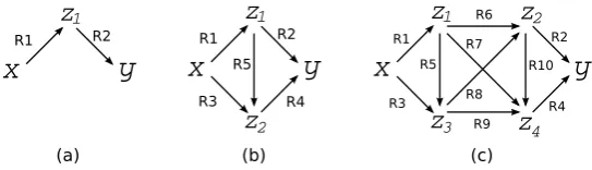
Figure 1. Defining new relations from networks of previously defined relations.
However, depending on the theory and kinds of definition we are exploring, we may wish to generalise the definition constructions that are allowed. Figure 1 illustrates how new relations can be constructed by composition (a),conjoined composition (b) andnetwork composition. In each case the variableszi are
existen-tially quantified. Conjoined composition allows one to constrain a conjunction of two composition operations by specifying a relation (R5) between the two existen-tially quantified variables. Case (c) is very general since the internal constraints
3. Exhaustive Incrementally Generated Relation Sets
3.1. Freely Generated Level 1 Relations from R
Let us consider the generation of relations from an arbitrary primitive relationR
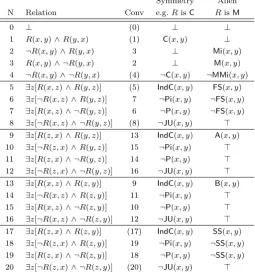
by means of the binary definition forming operations. After applying one binary relation combining operation, together with any number of the unary negation and converse operators, we get 42distinct Level 1 relations, including⊥(the empty relation) and >(the universal relation). Specifically, we get the 21 relations given in Table 1 (Column 2) and also the negations of these.
Among the 21 Level 1 relations, 7 relations are syntactically symmetric (the converse of a symmetric relation is itself) and the remaining 14 consist of 7 non-symmetric relations and their converses. When constructing Level 2 definitions, we need only consider combinations drawn from a set of 13 Level 1 relations (6 symmetric relations and 7 non-symmetric relations) plus the primitiveR. It is easy to check that relations⊥and>are not useful since however they are combined with another relation,R, the result is always equivalent to either⊥,>or some cognate ofR. From the 14 non-symmetric relations we only need consider one of each pair.
We have also analysed all ways in which two distinct relationsRandS can be combined by our binary relation generation operators. We do not give details here,
Symmetry Allen
N Relation Conv e.g.RisC RisM
0 ⊥ (0) ⊥ ⊥
1 R(x, y)∧R(y, x) (1) C(x, y) ⊥
2 ¬R(x, y)∧R(y, x) 3 ⊥ Mi(x, y) 3 R(x, y)∧ ¬R(y, x) 2 ⊥ M(x, y) 4 ¬R(x, y)∧ ¬R(y, x) (4) ¬C(x, y) ¬MMi(x, y) 5 ∃z[R(x, z)∧R(y, z)] (5) IndC(x, y) FS(x, y) 6 ∃z[¬R(x, z)∧R(y, z)] 7 ¬Pi(x, y) ¬FS(x, y) 7 ∃z[R(x, z)∧ ¬R(y, z)] 6 ¬P(x, y) ¬FS(x, y) 8 ∃z[¬R(x, z)∧ ¬R(y, z)] (8) ¬JU(x, y) >
9 ∃z[R(z, x)∧R(y, z)] 13 IndC(x, y) A(x, y) 10 ∃z[¬R(z, x)∧R(y, z)] 15 ¬Pi(x, y) >
11 ∃z[R(z, x)∧ ¬R(y, z)] 14 ¬P(x, y) >
12 ∃z[¬R(z, x)∧ ¬R(y, z)] 16 ¬JU(x, y) >
13 ∃z[R(x, z)∧R(z, y)] 9 IndC(x, y) B(x, y) 14 ∃z[¬R(x, z)∧R(z, y)] 11 ¬Pi(x, y) >
15 ∃z[R(x, z)∧ ¬R(z, y)] 10 ¬P(x, y) >
16 ∃z[¬R(x, z)∧ ¬R(z, y)] 12 ¬JU(x, y) >
[image:5.595.169.425.419.695.2]17 ∃z[R(z, x)∧R(z, y)] (17) IndC(x, y) SS(x, y) 18 ∃z[¬R(z, x)∧R(z, y)] 19 ¬Pi(x, y) ¬SS(x, y) 19 ∃z[R(z, x)∧ ¬R(z, y)] 18 ¬P(x, y) ¬SS(x, y) 20 ∃z[¬R(z, x)∧ ¬R(z, y)] (20) ¬JU(x, y) >
but it turns out that 96 distinct Level 1 relations can be constructed involving two different relations. A total of 178 Level 1 relations can be constructed using either justR justS or bothRandS.3
3.2. Constraints on Relations and the Domain
We now consider how to generate such specific sets in a systematic way. A systematic generation has advantages over an ad-hoc process, such as ensuring that every definition is at its lowest possible level and providing insight into the way a relation set builds up. The generation may be done by applying constraints on the logical properties of the relations involved and of the domain of entities to which they are applied to a freely generated set. The effect of such axioms is to shrink the class of semantically distinct relations. Each constraint corresponds to an equivalence relation on the set of freely generated relations. In terms of our generative definitional approach, we can consider these equivalence constraints in the following general cases:
3.2.1. The Case of a Symmetric Primitive Relation
Suppose we start with a symmetric primitive, such as the binary connection relation, C, of the RCC theory. We can easily identify the set of Level 1 definable relations of such a relation by considering how symmetry will give rise to logical equivalences among the freely generated Level 1 relations.
As the Table 1 (Column 4) shows for the case of theCrelation,0,2,3 are all equivalent to the empty relation⊥.1and4 are equivalent to the Level 0 relations
R and¬R respectively (Cand¬Cin the table); so as we stipulated above, they are considered to be Level 0. Furthermore, each of {5,9,13,17},{6,10,14,18}, {7,11,15,19}and{8,12,16,20} is a set of equivalent relations. Thus, symmetry of primitive relation, reduces the 21 relations given above to only 5 distinct Level 1 relations. Since, their negations are also Level 1, the total number of Level 1 relations definable from a symmetric relation is 10.
In constructing Level 2 relations from a symmetric relation, R, we only need consider relationsR,5,6 and8as constituents, because⊥is not useful and and7
is the converse of 6.
3.2.2. Reflexivity and Transitivity
Of the most commonly axiomatised properties of relations, symmetry seems to be the one that gives rise to the most significant reduction in the size of the levels in a generative definition survey, especially at the lower levels. Reflexivity and transitivity, do not give rise to any equivalences at levels 0 or 1. However, they do entail subsumptions between relations definable at level 1. Specifically: if R
is reflexive then the negated form of19is a subset ofR (e.g. in the RCC theory we haveP⊆C). IfR is transitive thenRis a subrelation ofRcomposed with R. These will give rise to significant reductions in the size of levels 2 and above, since they mean that certain intersections will be equivalent to the empty relation.
3We have 96 relations constructed using bothRandSand 42 with each ofRofS. 96 + 2∗42 =
3.3. Axioms of the domain as constraints
In addition to the general properties of the set of primitive relations, we may use a set of axioms to constrain their meaning and the domain of entities to which they apply. This will reduce the set of logically distinct definitions generated.
Allen and Hayes [2] gave an axiomatisation of temporal intervals using the relation meets Mas a primitive. For intervalsx, y,xmeets y, i.e.M(x, y), iff the end of xis simultaneous with the beginning of y. Using these axioms, we have proved that the previous definitions of Allen’s 13 temporal interval relations are equivalent to those that were given in [2]. Moreover, we show in Table 1 (Column 5) that, from the set of freely generated relations at Level 1, the relations 8,10,11,
12,14,15,16and20can be inferred from the axioms, being therefore equivalent to the universal relation within this domain. Any instance of relation1 would be inconsistent with the axioms, so it is equivalent to the empty relation.2and3are equivalent to the Level 0 relationsM(y, x) and M(x, y) respectively. Finally, the pairs (6,7) and (18,19) are equivalent to the negations of5and17respectively. Therefore, there are only 5 logically distinct new relations and their negations at Level 1.MMimeans that eitherxmeets withy or ymeets with x.
M
SS B FS
EQ
FBF SBS
F D
S
O
Level 1
[image:7.595.205.405.376.544.2]Level 4 Level 3 Level 2
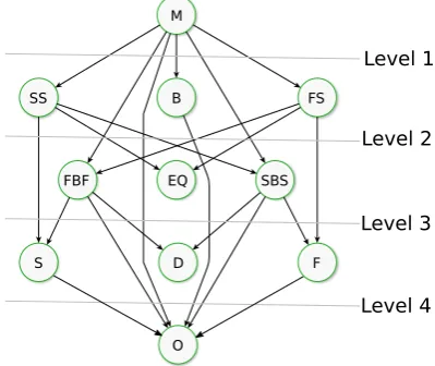
Figure 2. Definition derivation graph for Allen’s relations.
4. Generation of Allen’s 13 Basic Interval Relations
Allen’s Interval Calculus [2] specifies 13 jointly exhaustive and pairwise disjoint (JEPD) relations between temporal intervals:B(Before),M(Meet),O(Overlap),
S (Start),D(During), F(Finish); and their inverses:A(After),Mi,Oi,Si,Di,Fi; and EQ(Equal). UsingMas the primitive relation, Allen’s 13 temporal interval relations can all be defined by 4 or fewer binary relation combination operations. A number of intermediate relations are defined during the constructions:SS(Start at Same time), FS (Finish at Same time), SBS(x, y) (xstarts before y starts),
L0:M(x, y)
L0:Mi(x, y) ≡def M(y, x)
L1:B(x, y) ≡def ∃z[M(x, z)∧M(z, y)]
L1:A(x, y) ≡def B(y, x)
L1:SS(x, y) ≡def ∃z[M(z, x)∧M(z, y)]
L1:FS(x, y) ≡def ∃z[M(x, z)∧M(y, z)]
L2:EQ(x, y) ≡def SS(x, y)∧FS(x, y)
L2:SBS(x, y) ≡def ∃z[SS(x, z)∧M(z, y)]
L2:SAS(x, y) ≡def SBS(y, x)
L2:FBF(x, y) ≡def ∃z[M(x, z)∧FS(z, y)]
L2:FAF(x, y) ≡def FBF(y, x)
L2:BM(x, y) ≡def B(x, y)∨M(x, y)
L3:S(x, y) ≡def SS(x, y)∧FBF(x, y)
L3:Si(x, y) ≡def S(y, x)
L3:F(x, y) ≡def SBS(y, x)∧FS(x, y)
L3:Fi(x, y) ≡def F(y, x)
L3:D(x, y) ≡def SBS(y, x)∧FBF(x, y)
L3:Di(x, y) ≡def D(y, x)
L3:SBSFBF(x, y) ≡def
SBS(x, y)∧FBF(x, y)
L4:O(x, y) ≡def ∃z[S(z, y)∧F(z, x)]
L4:O(x, y) ≡def (alternatively) SBSFBF(x, y)∧ ¬BM(x, y)
L4:Oi(x, y) ≡def O(y, x)
5. Region Connection Calculus
The Region Connection Calculus (RCC) [18] is a first-order formalism based on regions and the primitive connection relation, C, axiomatised to be reflexive and symmetric. Two regionsx, yare connected (C(x, y) holds), if their closures share a point. Based on this relation, many spatial relations can be defined. Among them, a set of 8 JEPD relations are identified:DC(Disconnected),EC(Externally Connected),PO(Partially Overlap),TPP (Tangential Proper Part),NTPP (Non-Tangential Proper Part),TPPi(Inverse Tangential Proper Part),NTPPi(Inverse Non-Tangential Proper Part) and EQ (Equal). They are referred to as RCC-8, which is well-known in the field of qualitative spatial reasoning. The following 5 JEPD relations are referred to as RCC-5:DR(Discrete),PO,PP(Proper Part),
PPi(Inverse Proper Part) and EQ, which is a more granular version of RCC-8, which can be formed by disjoining DC and EC, and each pair of proper part relations. The basic theory can be extended by further definitions to create much more expressive vocabularies of relations (see e.g. [7,12]).
5.1. RCC Level 1 Relations Definable from C
Following the previous discussions and since Cis symmetric, Level 1 relations consist of only 5 logically distinct relations and their negations. As shown in Table 1 (Column 4), these are:
L1: ⊥(x, y) ≡def C(x, y)∧ ¬C(x, y)
L1: P(x, y) ≡def ∀z[C(z, x)→C(z, y)]
L1: Pi(x, y) ≡def ∀z[C(z, y)→C(z, x)]
L1: JU(x, y) ≡def ∀z[C(z, x)∨C(z, y)]
L1: IndC(x, y) ≡def ∃z[C(z, x)∧C(z, y)]
[image:8.595.124.473.155.289.2]of regions for which IndC6≡ >. For instance, the domain could be the nodes of a graph, withC(x, y) meaning that nodesxandy are connected by an edge.
5.2. Level 2 Relations Definable from C
Assuming that IndC≡ >, the only relations available for constructing Level 2 relations in RCC are: C, P, and JU. (Pi is also available, but is a cognate ofP, so need not be considered separately.) The fact that P⊆C also creates many equivalences. There are still a large number of possibilities. Specifically:
L2: C(x, y)∧ ¬P(x, y)
L2: C(x, y)∧ ¬P(y, x)
L2: C(x, y)∧JU(x, y)
L2: C(x, y)∧ ¬JU(x, y)
L2: ¬C(x, y)∧JU(x, y)
L2: ¬C(x, y)∧ ¬JU(x, y)
L2: P(x, y)∧JU(x, y)
L2: P(x, y)∧ ¬JU(x, y)
L2: P(y, x)∧JU(x, y)
L2: P(y, x)∧ ¬JU(x, y)
L2: ¬P(x, y)∧JU(x, y)
L2: ¬P(x, y)∧ ¬JU(x, y)
L2: ¬P(y, x)∧JU(x, y)
L2: ¬P(y, x)∧ ¬JU(x, y)
L2: O(x, y) ≡def
∃z[P(z, x)∧P(z, y)]
L2: POCR(x, y) ≡def
∃z[P(x, z)∧P(y, z)]
Many of the syntactically possible definitions yield relations equivalent to those at Level 0 or Level 1 and are not shown given here. In the context of the standard interpretation of RCC several of the given relations are not possible, or are equivalent to other relations. For instance,¬C(x, y)∧JU(x, y) is not possible unless the universe consists two or more separated components; and POCR(‘parts of a common region’) would be equivalent to >as long as every two region has a sum, or there is a universal region, of which every other region is a part.
5.3. Generation of RCC-5 and RCC-8
It turns out that all of the RCC-5 and RCC-8 relations can be generated using simple binary composition and Boolean operators. In fact all RCC-5 relations are generated at level 3 or less and all RCC-8 at level 4 or less:
L0: C(x, y) (Primitive)
L0: DC ≡def ¬C(x, y) (RCC-8)
L1: P(x, y) ≡def ∀z[C(z, x)→C(z, y)]
L1: Pi(x, y) ≡def P(y, x)
L2: EQ(x, y) ≡def P(x, y)∧P(y, x) (RCC-5, RCC-8)
L2: PP(x, y) ≡def P(x, y)∧ ¬P(y, x) (RCC-5)
L2: PPi(x, y) ≡def PP(y, x) (RCC-5)
L2: P-SC ≡def P(x, y)∨P(y, x) (thesymmetric closureofP)
L2: O(x, y) ≡def ∃z[P(z, x)∧P(z, y)]
L2: DR(x, y) ≡def ¬O(x, y) (RCC-5)
L3: EC(x, y) ≡def C(x, y)∧ ¬O(x, y) (RCC-8)
L3: PO(x, y) ≡def O(x, y)∧ ¬P-SC(x, y) (RCC-5, RCC-8)
L3: NTPP(x, y) ≡def ¬∃z[C(x, z)∧DR(z, y)] (RCC-8)
L3: NTPPi(x, y) ≡def NTPP(y, x) (RCC-8)
L4: TPP(x, y) ≡def PP(x, y)∧ ¬NTPP(x, y) (RCC-8)
L4: TPPi(x, y) ≡def TPP(y, x) (RCC-8)
(a) (b)
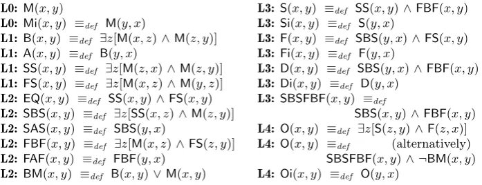
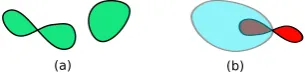
Figure 3. Cases ofnon-tangential partial overlap(NTPO). In (a) a red region is in two disjoint parts, one is part of and the other is disjoint from the cyan region. In (b) the yellow region has a hole, which is within the area covered by the blue region.
5.4. Defining Complement
This systematic strategy enables the selection of a definition at its lowest possible level, given that, through the generation process, a definition is only added to a level if there are no prior equivalences. As an example, consider the definition of Compl(x, y), meaning that x is the complement of y (i.e. the largest region that does not overlap y). The early RCC paper [18] contains a definition of a complement function, which implicitly defines a complement relation by:4
L5: Compl(x, y) ≡def ∀z[C(z, x)↔ ¬NTPP(z, y)]∧O(z, x)↔ ¬P(x, y)]
However, while searching the space of possible definitions, we found the following much simpler definition at level 3:
L3: Compl(x, y) ≡def JU(x, y)∧ ¬O(x, y)
5.5. Case Study of the NTPO Relation
The binary relation combining rules provide a systematic way of generating more complex relations from existing sets. The following sequence of definitions leads up to the definition ofnon-tangential partial overlap,NTPO, which occurs when the interior and exterior of one region both have intersections with the interior and exterior of another region, but boundaries of these two regions do not intersect. In other words, each region has a part within and a part outside the other, but their boundaries do not intersect. Two examples are illustrated in Figure 3.
L4: NTPP-SC(x, y) ≡def NTPP(x, y)∨NTPP(y, x) L5: Compo+(x, y) ≡def ∀z[TPP(z, x)→TPP(z, y)]
L6: R1(x, y) ≡def ∃z[PP(z, x)∧Compo+(z, y)]
L7: Compo(x, y) ≡def Compo+(x, y)∧ ¬R1(x, y)
L5: SDCB(x, y) ≡def DC(x, y)∨NTPP-SC(x, y)
L8: R2(x, y) ≡def ∀z[Compo(z, x)→SDCB(z, y)]
L9: R3(x, y) ≡def ∀z[Compo(z, x)→R2(y, z)]
L10: R4(x, y) ≡def ∃z[Compl(x, z)∧R3(z, y)]
L11: R5(x, y) ≡def ∃z[Compl(x, z)∧R4(y, z)]
L13: R6(x, y) ≡def R3(x, y)∨R4(x, y)∨R4(y, x)∨R5(x, y) L14: NTPO4(x, y) ≡def PO(x, y)∧R6(x, y)
4It is not entirely clear why this definition has both of these conjuncts. It seems that the
(a) (b)
Figure 4. (a) illustrates different types of component of a region. (b) Illustrates the ‘straddling’ relation. In this case the red region straddles (the boundary of) the light blue region.
Compo(x, y) means ‘xis a component of y’ — i.e. a maximal self connected part (or whole piece). A multi-piece region is equal to the sum of its components. Note thatCompo(x, x) holds just in casexis self connected (i.e. in a single piece). The definition ofCompo(x, y) also allows the case of a component that is connected by a one or more single points (in 2D) or line-like contacts (in 3D), as shown in Fig. 4(a). However, these different types of component can be distinguished by further definitions. Compo+(x, y) is read ‘xis a componential part of y’ and means thatxis a part ofy such thatxis the sum of one or more (possibly all) components of y. This means that xis the sum of any number of self connected parts ofy.R1(x, y) holds ifxhas aproper part that is a component ofy. It is used in combination with Compo+to defineCompo, since a single component cannot have a sum of components as a proper part.
NTPP-SCis thesymmetric closure ofNTPP.SDCB(x, y) may be read as ‘x’ and y’ are in a Simple DisConnected Boundary relationship’. This holds when eitherxandyare disconnected or one is a non-tangential proper part of the other. These are ‘simple’ cases where the boundaries ofxandydo not intersect. However, this relation does not cover all cases where boundaries do not intersect, because
SDCB requires that all components of region x stand in the same topological relation to region y (and vice versa). In the case where both regions are single component regions with no holes, they can have disconnected boundaries only if the relationSDCBholds. But if either region is multi-piece or has holes then there are more cases that SDCBdoes not cover, and will be explained below.
R2(x, y) holds when all components ofxstand in relationSDCBtoy. This is a generalisation ofSDCB(x, y), since it allows different components ofxto stand in different topological relations toy. ExpandingR2in the definition of R3, we have: ∀z1[Compo(z1, x)→[∀z2[Compo(z2, y)→SDCB(z2, z1)]]], which is equivalent to ∀z1∀z2[Compo(z1, x)∧Compo(z2, y)→SDCB(z1, z2)]. Hence,R3(x, y) holds if for
every component z1 of xand for every component z2 of y, SDCB(z1, z2) holds. R3(x, y) is a symmetric relation.
R4 and R5 are variants of R3 where we consider the relationship involv-ing components of the regions’ complements. So R4(x, y) holds if R3 holds between the complements of x and y. The definition of R5 can be rewrit-ten as ∃z1[Compl(x, z1)∧[∃z2[Compl(y, z2)∧R3(z2, z1)]] This is equivalent to ∃z1∃z2[Compl(x, z1)∧Compl(y, z2)∧R3(z2, z1)]. Hence,R5(x, y) holds ifR3holds
between the complement ofxand the complement ofy.R5is a symmetric relation.
R6(x, y) specifies 4 different cases where the boundaries of xand y do not intersect. NTPO4(x, y) is a specialisation of PO(x, y) such that R6(x, y) holds additionally. It is easy to see thatR6(x, y) is a symmetric relation, thusNTPO4(x, y) is also symmetric. However,NTPO4(x, y) still does not cover all the cases where
complement of it as x2, then every componentx3 of x2 must have a connected
boundary. Let us callx3aCCComponentofx.NTPO(x, y) is defined regarding their CCComponents. Let R7(x, y) be a relation which holds iff for everyCCComponent
x3 of x, for every CCComponent y3 of y, such that SDCB(x3, y3) holds. Then NTPO(x, y) ≡def PO(x, y)∧R7(x, y). By definition, NTPO(x, y) is symmetric. Below, we show thatR7is definable in a similar manner to R3andR5.
L9: R2c(x, y) ≡def ∃z[Compl(x, z)∧R2(z, y)]
L10: R3c(x, y) ≡def ∀z[Compo(z, x)→R2c(z, y)]
L11: R4c(x, y) ≡def ∀z[Compo(z, x)→R3c(y, z)]
L12: R5c(x, y) ≡def ∃z[Compl(x, z)∧R4c(z, y)]
L13: R7(x, y) ≡def ∀z[Compo(z, x)→R5c(z, y)]
L14: NTPO(x, y) ≡def PO(x, y)∧R7(x, y)
NTPO seems to be a natural specialisation ofPO; however, a long sequence of binary definitions is required to specify it. The complexity of the definition seems to arise because of the many topologically distinct ways in which NTPO
can occur. Our investigation of the construction of theNTPOdefinition according to our binary combination rules has revealed simpler definitions of the component relationships than had been previously given. However, due to the huge proliferation of possible relation definitions fromCat higher levels, we have not yet been able to exhaustively search for the shortest possible definition ofNTPO. There may well be a much more straightforward definition (perhaps via the ‘straddling’ relation shown in Fig. 4).
Indeed, if we allow the conjoined compositionoperation that was mentioned in Section 2.2, we can generate NTPO much more directly. First we define a boundary connectedness relationBC(x, y) by the following disjunction of conjoined compositions (arrows denote the directions of non-symmetric relations, e.g. TP):
C TPPi TPP
EC EC
x
y
z
12
z
C TPPi
TPP EC
EC
x
y
z
12
z
V
x
BC(
,y
)
defV
EQ(
x
,y
)
The two disjuncts correspond to the case wherexandyshare a common part of their boundary either from the same or opposite side of their boundaries. We then define NTPO(x, y) ≡def PO(x, y)∧ ¬BC(x, y).
6. Level-by-Level Analysis of Allen, RCC and other Relation Sets
intervals which are convex and linear on time. On the other hand, RCC’s domain is composed by convex and concave regions within multiple dimensions [12].
With automated generation of the Allen relations, the process of filtering semantically distinct relations from the freely generated set is hard because we need to compute equivalences with respect to rather complex axioms. However, this process will end at level 6, providing a finite set of relations. By contrast, the generation of RCC levels is initially much easier because the RCC axioms of symmetry and reflexivity enforce strong constraints by means of simple axioms, but the number of distinct relations grows increasingly through generations.
In future development of this kind of definitional analysis, we suggest the notion of agenerative definitional survey. This would be an exhaustive listing (relative to some precise specification of definitional level) of all relations definable up to a given definitional level, from a given primitive relation (or set of relations) in the presence of certain axiomatically specified constraints. The axiomatic constraints act as a filter, which reduces the number of semantically distinct relations at each level. A generative definitional survey may be regarded as a representation of compiled semantic knowledge. As such, it is similar to the composition tables
that are often used to facilitate reasoning with relational calculi. In fact, because composition is one of our definition construction operators, the composition table for any set of relations may be directly obtained from a sufficiently deep generative definitional survey that includes those relations.
We have some initial results regarding definitional surveys up to Level 2, using standard composition and the binary combination operators. Our approach is to first generate the freely definable relations of a level using Prolog, then identify equivalences using a combination of Mace4 and Prover9 [1]. Although, no longer state of the art, these are certainly sufficient to derive the first two levels arising with a number of commonly applied constraints. We initially attempt to find a model using Mace to check if a counter-example to the equivalence can be found; if not, we try to prove equivalence using Prover9. This method seems to be very effective. Our initial results are as follows:
Level free sym sym+ref Allen
0 4 2 2 4
1 42 10 10 10
2 5326 242 216
7. Summary and Further Work
In this paper we have considered the problem of generating relational calculi from a set of primitive relations, of which RCC and Interval Algebra are two well known examples. Whereas these calculi originally employed definitions constructed in an
There are a variety of directions in which this work could be taken further. Firstly, other relational calculi could be investigated, for example, the INDU calculus which extends the Interval Algebra [17] . Secondly, the approach could be applied to other definitional frameworks, for example relational algebra (in which RCC has also been defined [9]), or to Description Logic [6].
References
[1] Prover9 and Mace4. https://www.cs.unm.edu/~mccune/mace4/. Accessed 1st May 2016. [2] J F Allen and P J Hayes. A common sense theory of time. InProceedings 9th IJCAI,
pages 528–531, Los Angeles, USA, 1985.
[3] B Bennett. A categorical axiomatisation of region-based geometry. Fundamenta Informat-icae, 46(1–2):145–158, 2001.
[4] B Bennett, A Isli, and A G Cohn. When does a composition table provide a complete and tractable proof procedure for a relational constraint language? InProceedings of the IJCAI-97 workshop on spatial and temporal reasoning, Nagoya, Japan, 1997.
[5] S Borgo, N Guarino, and C Masolo. A pointless theory of space based on strong congruence and connection. InPrinciples of Knowledge Representation and Reasoning, Proceedings of KR-96, 1996.
[6] D Calvanese, M Lenzerini, and D Nardi. Description logics for conceptual data modelling. InLogics for Databases and Information Systems, chapter 1. 1998.
[7] A G Cohn, B Bennett, J Gooday, and N Gotts. RCC: a calculus for region based qualitative spatial reasoning. GeoInformatica, 1:275–316, 1997.
[8] E Davis, N Gotts, and A G Cohn. Constraint networks of topological relations and convexity.Constraints, 4(3):241–280, 1999.
[9] I D¨untsch and E Orlowska. A proof system for contact relation algebras. Journal of Philosophical Logic, 29:241–262, 2000.
[10] M Egenhofer. Reasoning about binary topological relations. InProceedings of the Second Symposium on Large Spatial Databases, SSD’91 (Zurich), pages 143–160, 1991.
[11] M Egenhofer and R Franzosa. Point-set topological spatial relations.International Journal of Geographic Information Systems, 5(2):161–174, 1991.
[12] N M Gotts. How far can we ‘C’? defining a ‘doughnut’ using connection alone. InPrinciples of KR: Proceedings of the 4th International Conference (KR94). Morgan Kaufmann, 1994. [13] L Henkin, P Suppes, and A Tarski. The Axiomatic Method — with special reference to
geometry and physics. North-Holland, Amsterdam, 1959.
[14] P Ladkin and R Maddux.Representation and reasoning with convex time intervals. 1988. [15] P Ladkin and R Maddux. On binary constraint problems.Journal of the ACM, 41(3):435–
469, 1994.
[16] T Laguna. Point, line and surface as sets of solids.Journal of Philosophy, 19:449–61, 1922. [17] A Pujari, GV Kumari, and A Sattar. INDU: an interval and duration network. InAdvanced
Topics in Artificial Intelligence, pages 291–303. Springer, 1999.
[18] D A Randell, Z Cui, and A G Cohn. A spatial logic based on regions and connection. In Proc. 3rd Int. Conf. on Knowledge Representation and Reasoning, pages 165–176, 1992. [19] J Renz and B Nebel. On the complexity of qualitative spatial reasoning: a maximal tractable fragment of the Region Connection Calculus. InProceedings of IJCAI-97, 1997. [20] R M Robinson. Binary relations as primitive notions in elementary geometry. InThe
Axiomatic Method (with special reference to geometry and physics), pages 68–85, 1959. [21] A Tarski. On the calculus of relations. Journal of Symbolic Logic, 6:73–89, 1941. [22] A Tarski. Foundations of the geometry of solids. InLogic, Semantics, Metamathematics,
chapter 2. Oxford Clarendon Press, 1956. trans. J.H. Woodger.
[23] A Tarski. Some methodological investigations on the definability of concepts. InLogic, Semantics, Metamathematics. Oxford Clarendon Press, 1956. trans. J.H. Woodger. [24] A Tarski and S Givant.A Formalization of Set Theory without Variables. Number 41 in