This is a repository copy of
System identification from multiple short-time-duration signals
.
White Rose Research Online URL for this paper:
http://eprints.whiterose.ac.uk/3555/
Article:
Anderson, S.R., Dean, P., Kadirkamanathan, V. et al. (2 more authors) (2007) System
identification from multiple short-time-duration signals. IEEE Transactions on Biomedical
Engineering, 54 (12). pp. 2205-2213. ISSN 0018-9294
https://doi.org/10.1109/TBME.2007.896593
[email protected] https://eprints.whiterose.ac.uk/
Reuse
Unless indicated otherwise, fulltext items are protected by copyright with all rights reserved. The copyright exception in section 29 of the Copyright, Designs and Patents Act 1988 allows the making of a single copy solely for the purpose of non-commercial research or private study within the limits of fair dealing. The publisher or other rights-holder may allow further reproduction and re-use of this version - refer to the White Rose Research Online record for this item. Where records identify the publisher as the copyright holder, users can verify any specific terms of use on the publisher’s website.
Takedown
If you consider content in White Rose Research Online to be in breach of UK law, please notify us by
System Identification From Multiple
Short-Time-Duration Signals
Sean R. Anderson*, Paul Dean, Visakan Kadirkamanathan
, Member, IEEE
, Chris R. S. Kaneko, and John Porrill
Abstract—System identification problems often arise where the only modeling records available consist of multiple short-time-duration signals. This motivates the development of a modeling approach that is tailored for this situation. An identification algorithm is presented here for parameter estimation based on minimizing the simulated prediction error, across multiple signals. The additional complexity of estimating the initial states corre-sponding to each signal is removed from the estimation algorithm. A numerical simulation demonstrates that the proposed algorithm performs well in comparison to the often-used least squares method (which leads to biased estimates when identifying systems from measurement noise corrupted signals). The approach is applied to the identification of the passive oculomotor plant; parameters are estimated that describe the dynamics of the plant, which represent the time constants of the visco-elastic elements that characterize the plant connective tissue.
Index Terms—Initial conditions, oculomotor plant, output error, parameter estimation, state-space.
I. INTRODUCTION
A
COMMON approach to system identification is to assume that the model structure corresponds to an autoregressive with exogenous inputs (ARX) description, for which parame-ters are estimated using least squares (LS) [1]. However, the LS method can lead to significant bias in the parameter estimates if the signals are corrupted by measurement noise [2]. There are limited conceivable scenarios where measurement noise-free signals are recorded in a physiological context; hence, use of the ARX model is often inappropriate (except where the noise model has the same poles as the system). Therefore, an output error model is utilized in the modeling problem discussed here as an alternative to the ARX model, which results in correct treatment of the measurement noise entering the system description.There is no closed-form solution for the output error model parameter estimation problem. Therefore, the parameters must be estimated via a nonlinear search. An estimate of the param-eters can be obtained by minimizing the simulated prediction
Manuscript received September 1, 2006; revised March 3, 2007. This work was supported by EPSRC (UK) grant GR/T10602/01 under their Novel Com-putation Initiative.Asterisk indicates corresponding author.
*S. R. Anderson is with the Neural Algorithms Research Group, Department of Psychology, University of Sheffield, Western Bank, Sheffield S10 2TP, U.K. (e-mail: [email protected]).
P. Dean and J. Porrill are with the Neural Algorithms Research Group, De-partment of Psychology, University of Sheffield, Sheffield S10 2TP, UK.
V. Kadirkamanathan is with the Department of Automatic Control and Sys-tems Engineering, University of Sheffield, Sheffield S1 3JD, U.K.
C. R. S. Kaneko is with the Department of Physiology and Biophysics, School of Medicine, University of Washington, Seattle, WA 98195-7290 USA.
Digital Object Identifier 10.1109/TBME.2007.896593
error (SPE) [1]. However, the SPE is significantly dependent on the initial system conditions for short time periods after excita-tion [3]. Therefore, if the initial condiexcita-tions are unknown, which is generally true if they are unobserved, then these should be es-timated along with the model parameters if the signal is of short time duration.
A further complication arises when modeling a system from multiple signals: the number of initial conditions to estimate in-creases in proportion to the number of experimental signals: an th-order system will have initial conditions corresponding to a single experimental signal; if there are experimental sig-nals available for modeling, then there will be additional parameters to estimate. There are many cases, arising especially in the biological sciences, where multiple short-time-duration signals are collected for the purposes of system identification, for instance, when modeling muscle dynamics [4], [5] and the oculomotor plant [6], [7].
This paper takes the approach of solving the output error model identification problem via a separable least squares (SLS) estimation algorithm [8], [9]. The optimal estimate of the initial states is rewritten as a function of the model parameters. This removes the additional computational burden of estimating the initial state vector corresponding to each signal. Specifically, the state-space output error (SSOE) model representation is used, which leads to natural inclusion of the unknown states.
The proposed SLS method is applied to the practical problem of identifying the passive oculomotor plant using multiple sig-nals. The modeling of the oculomotor plant dynamics is im-portant for a number of reasons, including relating eye move-ment to oculomotor firing patterns [10], [11] and also for under-standing the underlying algorithms governing eye-movement control [12], [13].
The identification of the oculomotor plant that is conducted here involves a reanalysis of signals that were previously mod-elled in [6], where a specialized estimation algorithm was de-veloped. The aim of applying the proposed SLS algorithm to the problem of modeling the oculomotor plant is to demonstrate that this generic method works successfully on a real-world problem, which is validated by reference to the previous study described in [6].
There are alternative approaches to solving the joint state-pa-rameter estimation problem, such as subspace methods [14], [15]. An advantage of the SLS approach proposed here is that it makes the parameterization of the model particularly straight-forward so that states and model parameters can be easily related to physical quantities of interest. For instance in the application demonstrated here (modeling of eye movement dynamics), the model states are the extensions of each visco-elastic element representing the connective tissue and the model parameters are
2206 IEEE TRANSACTIONS ON BIOMEDICAL ENGINEERING, VOL. 54, NO. 12, DECEMBER 2007
the poles relating to the time-constants of the aforementioned visco-elastic elements.
The paper is structured as follows. Section II reviews the LS method in the context of identifying systems from signals corrupted by measurement noise; motivation is then demon-strated for the approach of minimizing the SPE as an alter-native. Section III provides background on the use of SLS in system identification. The SLS approach to modeling multiple signals is derived in Section IV. The proposed method is ana-lyzed and compared with LS in Section V. In Section VI, the method is applied to the estimation of the parameters that char-acterize the passive oculomotor plant. The paper is concluded in Section VII.
II. PROBLEMMOTIVATION
This section demonstrates the bias inherent in using LS to estimate the parameters of a model from an output signal cor-rupted by measurement noise. The minimization of SPE is then shown to be an appealing alternative, which provides motivation for the parameter estimation approach subsequently developed in the later sections.
A. Parameter Estimation via LS
It is often assumed that the structure that describes a linear time-invariant system (in discrete-time) is that of an ARX model. In fact, if no process noise is present and the observed system output is corrupted by measurement noise, then the correct system description is the output error (OE) model [1]. The purpose of this background section is to demonstrate how the LS parameter estimation of an OE model is biased by measurement noise. The single-input single-output OE model is described as
(1) (2) where is the system output at time is the observed system output corrupted by measurement noise, is the system input, and is a zero-mean normally distributed white process noise signal.
A one-step-ahead prediction model (based on the ARX struc-ture) may be formed to estimate the model parameters from the observed signals, which is
for (3)
where is the one-step-ahead residual modeling error, is the number of data samples, and
(4) (5)
In order to track the influence of the measurement noise signal on the LS estimate, the prediction model (3) can be separated into
(6) where
(7) (8) This form of the prediction model immediately shows that the problem formulation is incorrect, for this system, because the prediction of the system output is partially dependent on mea-surement errors at previous sample times.
The parameter estimation cost function corresponding to the prediction model (6) is
(9)
Minimizing leads to the LS estimate
(10)
where
(11) where denotes expectation and each diagonal element of is the variance of the measurement noise, that is
. .. (12)
This analysis demonstrates that the LS estimate is biased, when estimating parameters from measurement noise corrupted signals, because the solution includes the additional term , which is related to the variance, or power, in the noise signal.
Intuitively, it may be supposed that for high SNR, the LS esti-mate will not incorporate significant bias. However, it is the case that if any of the singular values of are of similar magnitude to any of the singular values of , the parameter estimates will be significantly biased. This point is demonstrated on an example problem in Section V-B.
B. Parameter Estimation via Minimization of SPE
search). This is the method typically used to identify the output error model [1].
The minimization of SPE is accomplished by filtering the input sequence through a transfer function model of the system , which for short-duration signals is dependent on the parameter vector and the initial state
(13) The parameter vector and initial state can be updated by a nonlinear least squares routine, minimizing the simulated pre-diction error , which is defined as
(14) It is apparent that this approach does not suffer from the bias of the LS method because the recorded output variables are not used inpredictingthe model output, in contrast to (6). Instead, the recorded (noisy) output signal is only used to obtain the residual error ; the model predictions are obtained indepen-dently of the recorded output signal using the input sequence and the system model .
III. SEPARATING THEOPTIMIZATIONPROBLEM: MODEL
PARAMETERS ANDINITIALSTATES
The problem of estimating the model parameters and initial states is simplified by recognizing that for any given model pa-rameters the corresponding initial states can be obtained from a closed form solution. Therefore, an SLS problem can be con-structed, where the model parameters are estimated via non-linear least squares and the initial states are obtained via the use of a state-space prediction model [9].
A linear discrete-time invariant system can be represented by the SSOE model
(15) (16) where is the state transition matrix,
is the input matrix, is the measurement matrix, is the system state, is the system output, is the measurement error, is the system input, and is a vector of unknown model parameters.
The sequence of system outputs can be written as a function of the unknown parameter vector and the initial state vector
(17) where
(18) (19) (20)
(21)
..
. ... (22)
where and
otherwise (23) The sequence of measurement errors is assumed to be zero mean and normally distributed. Therefore, it is apparent from (17) that for any given parameter vector a closed-form solution can be obtained for the initial state vector .
When the matrix is unknown, the state-space prediction model defined in (17) may be separated further so that the matrix is linearly related to the output along with the initial state vector [9]. In practice, a control canonical form may always be used to represent an input-output system where the matrix is known. Furthermore, for multiple signals, the number of ini-tial conditions will usually be much greater than the number of parameters in the matrix. Thus, the main computational ben-efits (from a state-parameter estimation perspective) are derived from separating out the initial states, which is discussed further in the next section.
The parameter vector can be estimated using an iterative non-linear search routine where the direction of update is dependent at each iteration on the estimate of . The particular nonlinear search used in this investigation was a quasi-Newton method, where the gradient is estimated using a numerical update; see, for instance, [16] and [17].
IV. PARAMETER ANDSTATE ESTIMATION FROM
MULTIPLESIGNALS A. Problem Definition
The identification task is to estimate the single set of model parameters that describes the dynamic behavior of the system that generated all the available signals and the initial states cor-responding to each signal; that is, to minimize the cost function
(24) where is the SPE corresponding to all signals and is the stacked initial state vectors corresponding to each signal
(25) where is the number of signals.
2208 IEEE TRANSACTIONS ON BIOMEDICAL ENGINEERING, VOL. 54, NO. 12, DECEMBER 2007
B. Parameter and State Estimation
The model prediction error can be expressed using a prediction model that is similar to (17), which is augmented to include all signals,
(26) where the model that predicts the output corresponding to all signals is and
(27) . .. (28)
(29) Substituting (26) in (24) leads directly to the definition of the cost function
(30) Formulating the above optimization task as a separable least squares problem requires finding a closed-form solution for the optimal initial state vector as a function of . Taking the partial derivative of with respect to leads to
(31) Setting and solving for the optimal es-timate leads to
(32) where denotes the pseudoinverse of .
Substituting (32) in (30) has the desired effect of removing the unknown initial state vector from the cost function , leading to a new cost function that is only a function of the parameter vector, that is
(33) where
(34) The optimal model parameters are obtained by minimization of (33)
[image:5.594.288.552.70.263.2](35) Note that this minimization problem is not a function of the initial state vector. Hence, the number of parameters to estimate via a non-linear search is reduced from to just , where is the number of signals, is the system order and is the number of model parameters.
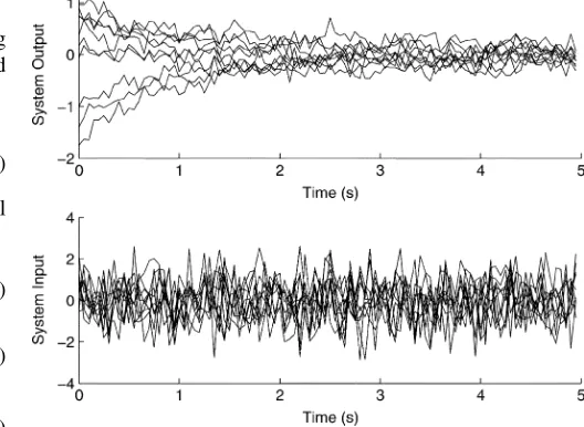
Fig. 1. One set of input/output training signals used in the test identification problem.
V. ANALYSIS OFSLS PARAMETERESTIMATION
ALGORITHMPERFORMANCE
This section describes the application of the SLS identifica-tion algorithm developed above to a test problem, focusing on the parameter estimation problem; a comparison is made with LS.
A. Problem Definition
The discrete-time test system was described in input–output form as
(36) A total of 10 signals were generated using a set of input records (normally distributed zero-mean white noise) and varying initial conditions in each case. The transfer function was mapped into state-space control canonical form (of system order ) for the straightforward inclusion of initial conditions; each initial state was defined as a random number, drawn from a uniform distribution in the range (0, 1).
To simulate measurement noise each signal was corrupted by normally distributed zero-mean white noise (adjusted to an SNR of 20 dB for each separate signal). The duration of the simulation was 5 s, and the sample rate was defined to be 20 Hz. The training signals are shown in Fig. 1.
To demonstrate the consistency of each estimation algorithm, the initial ten signals were duplicated 200 times with different measurement noise corruption. Each estimation algorithm (LS and SLS) was then applied to these different data sets. The LS estimate was obtained by concatenation of the regression matrix pertaining to each signal as described in [1].
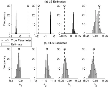
Fig. 2. Histograms that compare the true and estimated parameter values using (a) LS and (b) the SLS algorithm.
TABLE I
COMPARISON OFTRUE ANDMEANESTIMATED
PARAMETERVALUES
B. Parameter Estimation Results
The application of each estimation algorithm led to parameter estimates that were consistent. However, the LS method lead to parameter estimates that were consistently and significantly bi-ased (excepting the parameter , which may have been due to the fact that it was a gain term). In contrast, the application of the proposed SLS algorithm reduced the bias in the estimate con-siderably. The results of parameter estimation for each method are shown in Fig. 2 in the form of histograms. The mean values of the parameter estimates are given in Table I.
To emphasize the poor performance of LS at even very high SNR levels (as hypothesized in Section II), each estimation al-gorithm (LS and SLS) was applied to a similar problem as de-fined above, but varying the SNR (note that only one set of sig-nals was used at each level of SNR). The results confirmed that the LS estimate can be significantly biased at high SNR, whereas the SLS algorithm can reduce the bias to very small magnitudes at both low and high SNR. The results are shown in Fig. 3, in terms of RMSE in the parameter estimates.
Fig. 3. Accuracy of parameter estimates when varying SNR.
VI. MODELING OF THEOCULOMOTORPLANT
The modeling results presented here are compared to those previously presented in [6]. That method utilized the contin-uous-time system relationship , and hence was only useful in the case of modeling systems with zero input. The val-idation results presented in [6] show that the method was effec-tive in describing the system dynamics; therefore, the compar-ison of new results presented here provides a cross-validation of the generic SLS systems modeling algorithm developed above.
A. Data Collection
2210 IEEE TRANSACTIONS ON BIOMEDICAL ENGINEERING, VOL. 54, NO. 12, DECEMBER 2007
Fig. 4. Mechanical connectivity of the oculomotor plant.
extracellular electrophysiological recording techniques, but the nucleus itself had not been injected with ibotenic acid when these measurements were taken.
Following calibration of eye movements by requiring the animal to fixate targets at known eccentricities, the animal was lightly anaesthetized with ketamine ( mg/kg). Ketamine was chosen so that the animal would tolerate mechanical manipulation of the globe and because it is a dissociative anaesthetic and should thus minimize the affects on normal activity level in brainstem structures. Topical anaesthetic could not be used because completely alert animals do not tolerate manipulation of the globe even when it is anaesthetised. The exact dosage was titrated to the minimum level necessary to allow the animal to tolerate manipulation of the globe. It was low enough to avoid precipitating the vertical nystagmus that often accompanies higher doses (e.g., 25 mg/kg). If the threshold for vertical nystagmus was exceeded measurements were postponed until a future session. Horizontal nystagmus was never observed.
After a sufficient anaesthesia level was attained, the coiled eye was deviated manually with small forceps to between 15 and 45 either medial or lateral in the horizontal plane and abruptly released. Care was taken to avoid vertical deviation by monitoring eye position via the coil output. Trials were excluded if the return to resting position could be seen not to follow a smooth velocity trajectory due to the occurrence of a blink, sac-cade or slow eye movement. Eye position was sampled at 1 kHz.
B. Modeling
1) Model Structure: Knowledge of the physical system can lead to a useful representation of the system model in an identi-fication context. This section describes the formation of an ap-propriate model structure based on physical insight.
The connective tissue of the oculomotor plant is a viscoelastic structure [18], which can be represented by a small number of Voigt elements in series [6], [7], as described in Fig. 4. Fig. 4 shows the mechanical structure of the eye connectivity, where is a damping constant and is an elasticity constant (the time constant associated with the th Voigt element is ). The model representation of the system with zero input is defined in the state-space form as
[image:7.594.384.552.516.571.2](37) (38)
Fig. 5. Eye rotation data used for training and validation.
The states can be defined with physical significance; in this case the extension of a Voigt element. This requires the measured output (the extension of the muscle) to be the sum of the exten-sion of each individual Voigt element (that is, the states). This leads to a natural definition of the state-space matrices as
. .. (39)
(40) where the poles of the system, , for , in the dis-crete-time model are related to the time constants of the corre-sponding Voigt elements (in the continuous-time system model) by the relationship
for (41) where is the sample time.
To ensure that the model remained stable and nonoscillatory (a known property of the system), the parameter estimates were transformed within the search routine using the expression
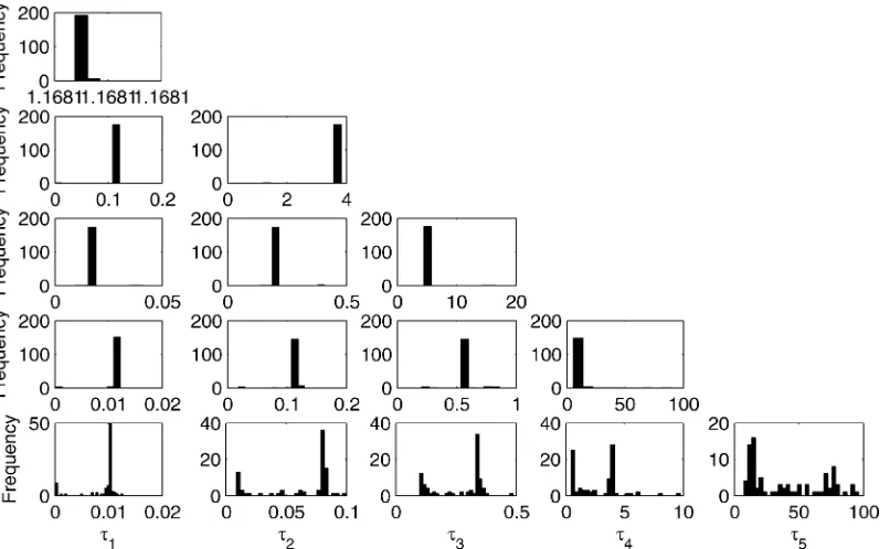
Fig. 6. Converged parameter estimates from 200 random initial values, corresponding to model orders from 1 to 5, where each row of histograms corresponds to a single model structure.
where was the transformed parameter vector; note that . In practice, this formulation of the problem led to improved numerical properties: the associated problem was due to the presence of a long system time constant, which cor-responded to a pole situated close to the edge of the unit circle. This pole would occasionally go unstable during the estimation procedure, probably because such a relatively long time con-stant acted like a concon-stant offset in the short term and therefore growth or decay (that is, instability or stability) of the pole was insignificant over the recording scale of the data.
2) Data Preprocessing: The resting position of the eye (in each case lateral to the primary position) was estimated from inspection of all the eye-position traces. Traces that were in-terrupted within 400 ms of release by discontinuities of slope (possibly corresponding to active components such as small sac-cades that are often associated with ketamine anaesthesia) were excluded from further analysis. Each remaining trace was fitted from the time of its maximum velocity, rather than from the time of release. In theory, these two times should coincide for a pure viscoelastic system released instantaneously, that is, the accel-eration time should be zero. However, in the actual traces, the time from release to peak velocity ranged from 8 to 20 ms, re-flecting an unknown combination of (small) globe inertia and the release time of the forceps opening. Fitting from the time of peak velocity was an attempt to avoid these complexities: The full set of signals are shown in Fig. 5. Training and validation data sets were formed by partitioning adjacent trials, resulting in a training set of five trials and a validation set of five trials.
[image:8.594.307.546.355.532.2]3) Modelling Results: The model structure detection problem for a real system is complicated by the fact that the optimal parameters for a given structure are unknown. The ap-proach taken in this investigation was to assess the consistency of the parameter estimates by starting the estimation algorithm at different values. In practice this was accomplished by se-lecting the initial poles randomly from a uniform distribution in
Fig. 7. RMSE corresponding to increasing model order.
the range (0, 1). This incorporated the known prior information about the system poles, that is, stable and real-valued. The esti-mation algorithm was run from 200 different starting estimates for each model order.
Fig. 6 displays the parameter estimates in the form of his-tograms for model orders to (where each row of histograms corresponds to a single model structure). It is ap-parent that there is a consistency in the estimates at each model order to ; at model order , the consis-tency begins to degrade, which may be due to the relative high order causing overfitting of the data, and hence redundancy in the system description.
2212 IEEE TRANSACTIONS ON BIOMEDICAL ENGINEERING, VOL. 54, NO. 12, DECEMBER 2007
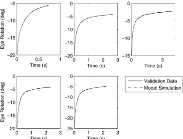
Fig. 8. Model prediction over validation data for the model of oculomotor plant dynamics.
system, evidence for which can be seen in Fig. 7, which shows the root mean square error (RMSE) of prediction for increasing model orders.
The model was validated in the time domain by verifying its prediction accuracy on the reserved independent data set; the model predicted output is shown in Fig. 8. The accuracy of the prediction demonstrates that this model was a good descriptor of the system.
The discrete-time state-space model was identified as
(43)
This model description corresponds to continuous-time domain time constants of s, s, s, and s.
These modeling results correspond closely to those presented in [6] in terms of both structure (4 visco-elastic units) and pa-rameter estimates, where the time constants were reported to be approximately 0.01 s, 0.1 s, 1 s, and 10 s. These results provide some validation as to the success of the generic modeling algo-rithm for multiple short-time-duration signals proposed here.
VII. CONCLUSION
An SLS parameter estimation method was derived that is useful for identifying a system from multiple short-time-duration signals. The proposed approach utilized an output error model; such a description naturally leads to a correct treatment of measurement noise, unlike the ARX model, which
was demonstrated to potentially lead to significant bias at even high SNR levels. Most conceivable physiological signals would contain measurement noise, hence the output error approach would appear to be widely applicable. The passive characteristics of the oculomotor plant were identified using the SLS algorithm; the results were validated by reference to a previous study. This demonstrated the utility of the proposed method because the oculomotor plant is a demanding system to identify, incorporating a wide range of time constants.
REFERENCES
[1] L. Ljung, System Identification—Theory for the User, 2nd ed. Upper Saddle River, NJ: Prentice-Hall, 1999.
[2] L. Ljung, “Initialisation aspects for subspace and output error identifi-cation methods,” presented at the 5th Eur. Control Conf., Cambridge, U.K., 2003.
[3] G. F. Franklin, J. D. Powell, and A. Emami-Naeini, Feedback Control of Dynamic Systems, 4th ed. Upper Saddle River, NJ: Prentice-Hall, 2001.
[4] K. Hunt, M. Munih, and N. N. Donaldson, “Investigation of the Ham-merstein hypothesis in the modeling of electrically stimulated muscle,” IEEE Trans. Biomed. Eng., vol. 45, no. 8, pp. 998–1009, Aug. 1998. [5] J. Bobet, E. R. Gossen, and R. B. Stein, “A comparison of models
of force production during stimulated isometric ankle dorsiflexion in humans,”IEEE Trans. Neural Syst. Rehabil. Eng., vol. 13, no. 4, pp. 444–451, 2005.
[6] S. Sklavos, J. Porrill, C. R. S. Kaneko, and P. Dean, “Evidence for wide range of time scales in oculomotor plant dynamics: Implications for models of eye movement control,”Vision Res., vol. 45, pp. 1525–1542, 2005.
[7] S. Sklavos, D. M. Dimitrova, S. J. Goldberg, J. Porrill, and P. Dean, “Long time-constant behavior of the coulomotor plant in barbiturate anesthetized primate,”J. Neurophysiol., vol. 95, no. 2, pp. 774–782, 2006.
[9] J. Bruls, C. T. Chou, B. R. J. Haverkamp, and M. Verhaegen, “Linear and non-linear system identification using separable least squares,” Eur. J. Control, vol. 5, pp. 116–128, 1999.
[10] A. F. Fuchs, C. A. Scudder, and C. R. S. Kaneko, “Discharge patterns and recruitment order of identified motoneurons and internuclear neu-rons in the monkey abducens nucleus,”J. Neurophysiol., vol. 60, no. 6, pp. 1874–1895, 1988.
[11] K. E. Cullen, H. L. Galiana, and P. A. Sylvestre, “Comparing extraoc-ular motoneuron discharges during restrained saccades and head-unrestrained gaze shifts,”J. Neurophysiol., vol. 83, pp. 630–637, 2000. [12] P. Dean, J. Porrill, and J. V. Stone, “Decorrelation control by the cerebellum achieves oculomotor plant compensation in simu-lated vestibulo-ocular reflex,” Proc. R. Soc. Lond. B, vol. 269, pp. 1895–1904, 2002.
[13] P. M. Blazquez, Y. Hirata, S. A. Heiney, A. M. Green, and S. M. High-stein, “Cerebellar signatures of vestibulo-ocular reflex motor learning,” J. Neurosci., vol. 23, pp. 9742–9751, 2003.
[14] M. Verhaegen, “Subspace model identification part 3. Analysis of the ordinary output-error state-space model identification algorithm,”Int. J. Control, vol. 58, no. 3, pp. 555–586, 1993.
[15] B. R. J. Haverkamp, “State space identification: Theory and practice,” Ph.D. dissertation, Technical Univ. Delft, Delft, The Netherlands, 2001.
[16] D. F. Shanno, “Conditioning of quasi-Newton methods for function minimization,”Math. Computat., vol. 24, pp. 647–656, 1970. [17] G. A. F. Seber and C. J. Wild, Nonlinear Regression. New York:
Wiley, 2003.
[18] D. A. Robinson, “The mechanics of human saccadic eye movement,” J. Physiol., vol. 174, pp. 245–264, 1964.
Sean R. Andersonwas born in Reading, U.K., in 1979. He received the M.Eng. degree in control systems engineering from the Department of Auto-matic Control and Systems Engineering, University of Sheffield, U.K., in 2001 and the Ph.D. degree from the Department of Chemical and Process Engineering in 2005.
He is currently a Research Associate in the Neural Algorithms Research Group, Department of Psychology, University of Sheffield, where he studies the central nervous system, using systems engineering techniques to interrogate methods of biological adaptive control. His research interests include identification of continuous- and discrete-time dynamic systems, nonlinear systems modeling, and the study of adaptive control in biological systems.
Paul Deanreceived the M.A. degree in physiology with psychology from the University of Cambridge, U.K., and the D.Phil. degree from the University of Oxford, U.K.
He is currently a Professor in the Department of Psychology at the University of Sheffield, U.K., and is a member of the recently established Centre for Signal Processing in Neuroimaging and Systems Neuroscience. His major research interest is in producing computational models of neural systems that are based on both biological data and current developments in control engineering, signal processing, and robotics. These models are intended to serve as a vehicle for two-way communication between biological and physical sciences, allowing roboticists to use new discoveries in biology, and biologists to interpret their findings in the light of current developments in signal processing.
Visakan Kadirkamanathan(S’89–M’90) was born in Jaffna, Sri Lanka He received the B.A. and Ph.D. degrees from the Department of Engineering, Univer-sity of Cambridge, U.K.
Previously, he has held Research Associate posi-tions at the University of Surrey, U.K., and the Uni-versity of Cambridge, U.K. In 1993, he joined the University of Sheffield as a Lecturer, where he is cur-rently a Professor in the Signal Processing and Com-plex Systems Research Group of the Department of Automatic Control and Systems Engineering. He has coauthored a book on intelligent control titledFunctional Adaptive Control: An Intelligent Systems Approach(London, U.K.: Springer, 2001) and has published more than 120 papers in refereed international journals and proceedings of inter-national conferences. His research interests include nonlinear signal processing and control, optimization and decision support, signal and fault detection and neural networks with applications in biomedical systems modeling, aircraft en-gine health monitoring, and systems biology.
Prof. Kadirkamanathan is the Co-Editor of theInternational Journal of Sys-tems Scienceand has served as an Associate Editor for the IEEE TRANSACTIONS ONNEURALNETWORKSand the IEEE TRANSACTIONS ONSYSTEMS, MAN AND
CYBERNETICS, PARTB.
Chris R. S. Kaneko received B.A. degrees in psychology and zoology from the University of Cal-ifornia at Los Angeles in 1968 and the M.A. degree in psychology and the Ph.D. degree in zoology from the University of Iowa, Iowa City, in 1970 and 1973, respectively.
He was a Postdoctoral Fellow in the Division of Cellular Neurobiology of the Department of Neuroscience at Einstein College of Medicine and Neurophysiology at the University of Washington, Seattle. He is currently a Research Scientist in the Department of Physiology and Biophysics of the University of Washington. His research interests are oculomotor system neurophysiology and saccadic eye movement control, in particular.