Verification of BOUT++ by the method of manufactured solutions

This is a repository copy of

Verification of BOUT++ by the method of manufactured

solutions

.

White Rose Research Online URL for this paper:

http://eprints.whiterose.ac.uk/101319/

Version: Accepted Version

Article:

Dudson, Benjamin Daniel orcid.org/0000-0002-0094-4867, Madsen, Jens, Omotani, John

Tomotaro et al. (3 more authors) (2016) Verification of BOUT++ by the method of

manufactured solutions. Physics of Plasmas. 062303. ISSN 1089-7674

https://doi.org/10.1063/1.4953429

[email protected] https://eprints.whiterose.ac.uk/ Reuse

Items deposited in White Rose Research Online are protected by copyright, with all rights reserved unless indicated otherwise. They may be downloaded and/or printed for private study, or other acts as permitted by national copyright laws. The publisher or other rights holders may allow further reproduction and re-use of the full text version. This is indicated by the licence information on the White Rose Research Online record for the item.

Takedown

If you consider content in White Rose Research Online to be in breach of UK law, please notify us by

Verification of BOUT++ by the Method of Manufactured Solutions

B.D.Dudson,1,a) _J.Madsen,2 _J.Omotani,3 _P.Hill,1 _L.Easy,1, 4 _{and M.Løiten}2

1)_{York Plasma Institute, Department of Physics, University of York, Heslington,}

York YO10 5DD, UK

2)_{Department of Physics, Technical University of Denmark, DK-2800 Kgs. Lyngby,}

Denmark

3)_{Department of Physics, Chalmers University of Technology, SE-412 96 G¨oteborg,}

Sweden

4)_{CCFE, Culham Science Centre, Abingdon, OX14 3DB,}

UK

BOUT++ is a software package designed for solving plasma fluid models. It has

been used to simulate a wide range of plasma phenomena ranging from linear

sta-bility analysis to 3D plasma turbulence, and is capable of simulating a wide range

of drift-reduced plasma fluid and gyro-fluid models. A verification exercise has been

performed as part of a EUROfusion Enabling Research project, to rigorously test

the correctness of the algorithms implemented in BOUT++, by testing

order-of-accuracy convergence rates using the Method of Manufactured Solutions (MMS).

We present tests of individual components including time-integration and advection

schemes, non-orthogonal toroidal field-aligned coordinate systems and the shifted

metric procedure which is used to handle highly sheared grids. The Flux

Coordi-nate Independent (FCI) approach to differencing along magnetic field-lines has been

implemented in BOUT++, and is here verified using the MMS in a sheared slab

configuration. Finally we show tests of three complete models: 2-field

Hasegawa-Wakatani in 2D slab, 3-field reduced MHD in 3D field-aligned toroidal coordinates,

and 5-field reduced MHD in slab geometry.

PACS numbers: 52.25.Xz, 52.65.Kj, 52.55.Fa

I. INTRODUCTION

The BOUT++ code1,2 _{is an open source toolkit for the simulation of plasma models.}

Its applications include the study of plasma transients including Edge Localised Modes and

filament / blob transport, and turbulence in magnetised plasma devices. Here we present a

rigorous code verification exercise3,4 _{of the BOUT++ core algorithms and numerical}

meth-ods, using the Method of Manufactured Solutions (MMS)3,5_{. Code verification is a process}

of checking that the chosen set of partial differential equations is solved correctly and

con-sistently, and is a purely mathematical exercise. Code verification is not concerned with

verifying that the chosen numerical methods are appropriate for the chosen set of equations.

Code verification is also not concerned with testing the ability of a given model to explain

experimental observations. This testing is dealt with in the subsequent validation process.

Code verification tests typically rely on a known solution against which to check the result

(the Method of Exact Solutions). In relatively simple geometries (e.g. slabs or cylinders)

and equations (usually linearised) an analytical solution can sometimes be found, and this

kind of test is used to verify BOUT6 _{and BOUT++}1 _{as part of a test suite, run regularly}

to reduce the chances of errors being introduced. The requirement that there be an

analyt-ical solution restricts the usefulness of the tests, as the code cannot be verified for realistic

geometries and problems of interest, where no such exact solution exists.

The Method of Manufactured Solutions (MMS)3,5 _{provides a method by which a}

simu-lation code can be verified in general situations, even where analytic solutions cannot be

found. This is done by imposing a known “manufactured” solution, and adding sources to

the equations such that the manufactured solution is an exact solution to the modified set

of equations. The manufactured solution and therefore also the source can be composed of

primitive analytical functions sin, cos, tanh etc. which can be evaluated with a very high

accuracy, typically double floating point precision. The difference between the numerically

calculated solution and the “exact” manufactured solution provides the numerical error.

The scaling of the numerical error with the numerical spatial resolution is known a priori,

and hence any deviation from the theoretical scaling must be due to code inconsistencies or

errors. The MMS is a very general technique, which has been used to verify a wide range of

engineering codes, particularly in the fluid dynamics community7_{. MMS has been applied to}

simulations9_{, and has recently been applied to the GBS turbulence code}10_{and tokamak edge}

simulations11_.

As in10_{, here we focus on order-of-accuracy tests as they provide the most rigorous test of}

numerical implementation4_{. In section II we describe in more detail the MMS procedure, and}

the changes made to BOUT++ to facilitate its routine use. BOUT++ simulations typically

employ non-orthogonal curvilinear coordinate systems, which are described in section III

along with the method used to perform tests in these coordinates. Individual components of

BOUT++ are first tested independently, including time integration schemes in section IV A,

advection schemes in section IV B, and operators for wave and diffusion equations along

magnetic fields in section IV C. Coordinate systems are then tested in section IV E. In

section V complete models are tested, in which these components are combined: The

2-field Hasegawa-Wakatani model of drift-wave turbulence in section V A; a 3-2-field reduced

Magnetohydrodynamics (MHD) model in section V B; and a 5-field reduced MHD model

similar to that in10 _{is tested in section V C.}

All source code, input files, and scripts needed to produce the figures and results in

this paper are publicly available as part of the BOUT++ development repository at

https://github.com/boutproject/BOUT-dev, revision 83c1f53. Due to automation of

the testing procedure (section II), most results and figures in this paper can be reproduced

by running a single Python script. The location of these scripts will be specified relative to

the root of the git repository.

II. TESTING FRAMEWORK

The BOUT++ code is not limited to a single set of equations, but has been developed

to allow an arbitrary number of evolving fields, and input of custom evolution equations

in a form close to mathematical notation (see1,2 _{for details). This flexibility presents a}

challenge for verification, due to the large number of possible combinations of operators and

settings such as boundary conditions, which could be employed. Fortunately, as pointed

out in5_{, only mutually exclusive settings and operators need be independently tested, not}

all possible combinations of options. This still requires a relatively large number of tests

to adequately cover the code components, and to verify each model. The process of MMS

to be specified in an input text file. This allows the same code to be tested with different

inputs, and new tests to be created more easily. Here we briefly outline the MMS procedure,

before describing the mechanisms implemented in BOUT++ to carry out MMS testing.

Time integration codes such as BOUT++ evolve a set of nonlinear equations for quantities

f, e.g. for a two field model evolving particle density and temperature f = {n, T}. The

system of equations is solved using the Method of Lines, and can be written in a general

form as:

∂f

∂t =F f

(1)

where F (·) is a nonlinear operator which contains discretised differential operators in the

spatial dimensions. In order to test the correctness of the numerical implementation, a

time-dependent function fM(t) is chosen (manufactured) using a combination of primitive

mathematical functions which can be evaluated to machine precision. Manufactured

solu-tions should be chosen so that they exercise all parts of the code, so should be varying in

time and all spatial dimensions. Ideally the magnitude of the terms in the equations solved

should be comparable, so that the error in one does not dominate over the others. Since

derivatives of the solution will be taken numerically, the solution should also be smooth.

Where the domain is periodic, such as toroidal angle in tokamak simulations, the

manufac-tured solutions must also be periodic in those directions. A detailed discussion of selection

criteria for manufactured solutions can be found in5_.

The manufactured functionfM _{is now inserted into the functionF (·) and} ∂fM

∂t to calculate

a source function S analytically:

S(t) = ∂f

M

∂t −F f

M

(2)

The function F (·) is typically composed of a combination of algebraic operations and

dif-ferential operators. This results in a closed analytic form for F fM

even when F(·) is

nonlinear or evaluated in non-orthogonal curvilinear coordinate systems, since fM is only

ever differentiated with respect to time and spatial coordinates, and not integrated. In some

cases F (·) contains integrals, as in the models tested in section V, where the potential φ

is calculated by integrating the vorticity. These integrals may not have a closed analytic

solution, and so in these cases a solution to the integral (potential φ) is manufactured, and

Here the symbolic packages Mathematica and the Sympy library12_{were used to calculate}

source functions. Both can generate representations of the resulting expressions which can

be copied directly into source code or text input files. For large sets of equations such as

those in section V C this is essential in order to avoid introducing errors.

The system of equations to be solved numerically is now modified to:

∂f

∂t =F f

+S(t) (3)

so that the function fM _{is an exact (manufactured) solution of equation 3. Since S has}

been calculated analytically, it can be evaluated to within machine precision at any desired

time, and passed to the time integration routines. At the start of the simulation t = 0

the state is set to the manufactured solution f = fM (t = 0). The simulation time is then

advanced to some later timet= ∆t, at which point the numerical solutionf is compared to

the manufactured solution fM(t = ∆t). The norm of the difference between the numerical

solution and the manufactured solution ǫ =

f−fM

at t = ∆t then gives a measure of

the error in the numerical solution, which should converge towards zero as the spatial and

temporal mesh is refined. Note that in order to obtain convergence in the solution of a

time-dependent Partial Differential Equation (PDE), both the spatial and temporal mesh

(time step) must be refined13_{. In general separating the spatial and temporal convergence is}

non-trivial, but in section IV D we use a slightly different procedure than outlined above, to

verify spatial convergence and boundary conditions independently of temporal convergence.

Boundary conditions must also be modified for testing with the MMS. A Dirichlet

bound-ary condition on a quantity n (e.g. particle density), for example, must be modified to set

the solution equal to the time-varying manufactured solution nM _{on the boundary:}

n(boundary) =nM_{(boundary, t) (4)}

Similarly for Neumann boundary conditions:

∂n

∂x (boundary) = ∂nM

∂x (boundary, t) (5)

More complex boundary conditions such as sheaths, which couple multiple fields together,

can be treated by adding a source function as for the time integration equation 3. The

boundary conditions applied to all fields now become time-dependent, and must be evaluated

In order to test a numerical model using the Method of Manufactured Solutions, three

analytic function inputs are therefore required for each evolving field (e.g. density n,

tem-perature T, ...):

1. A manufactured solution

2. A source function calculated from equation 2 using a symbolic package like SymPy

3. Analytic expressions for boundary conditions

As described in2_{, BOUT++ contains an expression parser which evaluates analytic}

expres-sions in input files. This was added as a convenient means to specify initial conditions, but

has been extended and adapted for use in MMS testing. Once MMS testing is enabled by

setting a flag in the input, BOUT++ reads a manufactured solution from the input for each

evolving variable, using it to initialise the variable and to calculate an error at each output

time; a source function is read and used to modify the time derivatives which are passed

to the time-integration code; and expressions for boundary conditions are evaluated at the

required times. All of this machinery is independent of the specific model, and in most cases

does not require any modification of the problem-specific code1_{. The form of the analytic}

expressions is of course problem specific, but once calculated, a BOUT++ executable can

be tested using MMS and then used to perform physics simulations without recompiling,

only changing the input file. This automation of the testing process aims to lower the

bar-riers to routine testing of BOUT++ simulation models using the Method of Manufactured

Solutions.

III. COORDINATE SYSTEMS

In strongly magnetized plasmas the characteristic gradient length scales parallel to the

magnetic field are often much longer than the perpendicular length scales. This scale

sepa-ration is often exploited in numerical simulation to reduce the computational cost by using

a coarser discretisation in the direction parallel to the magnetic field. A widely used

ap-proach is to express the model equations in magnetic field-aligned, curvilinear coordinates.

1 _{The only code changes required for MMS testing are Laplacian inversions, which currently require some}

In most previous BOUT++ simulations1 _{we have used the so-called ballooning coordinates.}

Starting from orthogonal toroidal flux coordinates14 _{(ψ, θ, ζ) with radial flux-surface label}

ψ, poloidal angle θ, and toroidal angle ζ, the coordinates are transformed to field-aligned

ballooning coordinates (x, y, z)15

x=ψ y=θ z =ζ−

Z θ

θ0

νdθ ν = Bζr

BθR

(6)

where Bζ and Bθ are the toroidal and poloidal magnetic field components, r is the minor

radius, R is the major radius, and ν is the local magnetic field-line pitch. Moving along y

at fixed x and z follows the path of a field-line in both θ and ζ. The covariant basis vector

(the vector between grid-points) is1_:

~ex =

1 RBθ

~_{ˆeψ+IR~ˆeζ (7a)}

~ey =

hθ

Bθ

~

B (7b)

~ez =R~ˆeζ (7c)

where~eˆare the unit vectors in the original orthogonal toroidal (ψ, θ, ζ) coordinate system,

and I =R _∂ν

∂ψdθ is the integrated shear. The magnetic field is given by B~ =∇z× ∇x, and

so the derivative along the magnetic field reduces to a simple partial derivative B~ · ∇ =

∇z × ∇x · ∇y∂y. Since fluctuations typically have long wavelengths along field-lines, a

lower resolution can be used in this parallely coordinate, with a corresponding reduction in

computational resources, both run time and memory.

In order to reduce the deformation of the coordinates caused by magnetic shear I (see

~ex in equation 7), a shifted metric method16,17 is usually used, a discussion of which can

be found in1 _{and more recently in}18_{. At each y = const plane, a local coordinate system}

is defined in which x and z are orthogonal. Mapping between these local coordinates and

the global field-aligned coordinates can be done using Fast Fourier Transforms (FFTs) in

the toroidal (ζ, z) direction. As implemented in BOUT++, this procedure has no effect on

differencing in the parallel direction, but differencing in x is modified by shifting quantities

inz using FFTs before calculating finite differences.

A toroidal coordinate system for MMS testing is generated by first specifying the path of

magnetic field lines in poloidal and toroidal angle. The poloidal magnetic field can then be

have relatively compact closed forms. The formula used here for the toroidal angle ζ as a

function of the radial (flux) coordinateψ and poloidal angle θ is:

ζ =q(ψ) [θ+ǫsinθ] (8)

where q(ψ) is the safety factor, which is taken to be a parabolic function of ψ varying

between 2 and 3 in sections IV E and V B. ǫ =r/R0 is the inverse aspect ratio, here taken

to beǫ= 0.1. From this, the field line pitch is calculated as

ν =q(ψ) [1 +ǫcosθ] (9)

A fixed value of the poloidal current function f =BζR and minor radius r = ǫR0 is used,

and the major radius of a field line varies asR =R0+rcosθ. Equation 9 is then rearranged

to give an expression for the poloidal field. The integrated shear is calculated from the

differential of the field-line toroidal angleζ with respect to ψ:

I =

Z θ

θ0

∂ν ∂ψdθ=

∂q(ψ)

∂ψ [1 +ǫcosθ] (10)

The resulting covariant and contravariant metric tensors have the same non-zero

pat-tern as in simulations of real devices, and elements of the covariant metric tensor vary in

both radial and poloidal coordinates15_{. Differencing operators parallel and perpendicular}

to the magnetic field are tested in this coordinate system in section IV E, and a 3-field

electromagnetic reduced MHD model is verified in this coordinate system in section V B.

A. Flux Coordinate Independent scheme

Recently a new approach to plasma turbulence simulations has been developed18,19_{, and}

work is ongoing to implement this scheme in several simulation codes. We have implemented

this Flux Coordinate Independent (FCI) scheme in BOUT++, enabling the development of

complex turbulence models in arbitrary magnetic geometry. By assuming that the poloidal

plane equals the plane perpendicular to the magnetic field, complex non-orthogonal

curvilin-ear field-aligned flux coordinates do not need to be used in the perpendicular direction, but

can use simple geometries (e.g. Cartesian). Here we verify that these numerical schemes

have been implemented correctly for a sheared slab geometry. Further development and

Magnetic field_B

Interpolation

FIG. 1. Flux Coordinate Independent (FCI) scheme. To calculate the derivative along the

mag-netic field at grid cells (large solid circles), field-lines are followed in both directions to points on

neighbouring planes of grid cells (small open circles). Values at these points are found by high-order

interpolation using nearby points (blue box).

The Flux Coordinate Independent scheme, as implemented in BOUT++, employs 3rd

-order Hermite polynomial interpolation in the plane perpendicular to the magnetic field, and

2nd_{-order central differencing along the magnetic field. The idea is illustrated in figure 1:}

The grid is constructed to be dense in planes perpendicular to the magnetic field and sparse

along the magnetic field, since from physical arguments we expect the solutions to vary

slowly along magnetic field-lines (k|| ≪k⊥). To calculate derivatives of a quantity f along

magnetic fields, the magnetic field is first followed from each grid point onto neighbouring

planes; values of f on neighbouring planes are then interpolated onto these intersection

locations. This gives the value of f at 3 points along the magnetic field (the starting

grid point, and one point along the field in each direction), which is sufficient to calculate

second-order accurate first or second derivatives using central differencing. If higher order

derivatives are required, then the magnetic field could be followed to calculate intersections

with further planes. There are subtle issues with this scheme which will not be addressed

here, and are left to future work: the treatment of boundary conditions where magnetic

field-lines intersect material surfaces, and time-evolving magnetic fields where the mapping

efficiency of the scheme in terms of the computing time required for high-order interpolation

is also important in determining the best overall scheme to employ, and is also left to future

work.

IV. RESULTS

Since operators can be tested and verified independently (see5 _{and discussion in}

sec-tion II), a suite of smaller tests is generally more useful than a test which combines

every-thing together. Whole models are tested in section V, but require considerable computing

resources to run, and if one of these fails then it is difficult to know where the error lies.

Tests of individual components can run in minutes on a desktop, rather than hours on a

su-percomputer, and a test failure provides better guidance as to the location of the error. The

difficulty is in the large number of tests needed to ensure coverage: Here we verify the

ma-jor components of BOUT++, including time integration schemes (section IV A), advection

operators (section IV B), central schemes for wave and diffusion equations (section IV C),

and the curvilinear coordinate system used for tokamak simulations (section IV E). Other

components, such as calculation of potential φ from vorticity, are verified as part of full

models (section V), and development of individual tests for these components is a matter of

ongoing work.

A. Time integration

Several explicit and implicit time integration schemes are implemented in BOUT++,

allowing users to choose at run-time which scheme to use. Methods tested are the Euler,

RK420_{, a multi-step method derived by Karniadakis et al}21,22_{, and a third-order Strong}

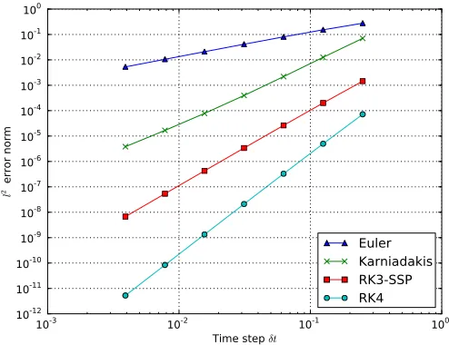
Stability Preserving Runge-Kutta method (RK3-SSP)23_{. Results obtained by integrating} ∂f

∂t =f between t= 0 and t = 1 are shown in figure 2. Other functions such as ∂f

∂t = cos(t)

have also been tested, resulting in the same convergence rate.

The Euler, RK3-SSP and RK4 methods all reproduce their expected convergence rates

(first, third, and fourth order in δt respectively), and so can be considered verified. The

Karniadakis scheme is expected to be third order accurate, but only second order convergence

10-3 ₁₀-2 ₁₀-1 ₁₀0

Time step δt

10-12

10-11

10-10

10-9

10-8

10-7

10-6

10-5

10-4

10-3

10-2

10-1

100

l

2 er

ror

no

rm

Euler Karniadakis RK3-SSP RK4

FIG. 2. Error norm for explicit time integration schemes. Measured convergence rates based on

the two highest resolution cases are: 0.995 (Euler), 2.13 (Karniadakis), 3.00 (RK3-SSP), and 3.99

(RK4). Script:examples/MMS/time/runtest

At each step the value of f and its time derivative at two previous timesteps are required,

and so to start the simulation these previous steps are constructed using Euler’s method.

This results in an O(δt2_{) error, reducing the overall convergence to second order in δt.}

Time integration in BOUT++ simulations is typically done using implicit adaptive

Jacobian-Free Newton Krylov (JFNK) schemes, provided by either the SUite of

Nonlin-ear and Differential/ALgebraic equation Solvers (SUNDIALS24_{) or the Portable, Extensible}

Toolkit for Scientific Computation (PETSc25,26_{). These use adaptive order and adaptive}

timesteps in order to achieve a user-specified tolerance, and so are difficult to validate using

the MMS method. Here we take as given that the time integration methods in these libraries

are implemented correctly, and use SUNDIALS for time integration in the remainder of this

paper with a relative tolerance of 10−8 _{and absolute tolerance of 10}−12_{. These small}

toler-ances are used so that the spatial discretisation error we are interested in dominates over

B. Advection schemes

A key component of drift-reduced plasma simulations are operators for drifts across

mag-netic field-lines. These can be written in the form of an advection equation, or as a Poisson

bracket. For example the E ×B drift of a scalar quantity f (e.g. density), due to an

electrostatic potential φ is:

∂f

∂t =−

1

B~b× ∇φ· ∇f =−[φ, f] (11)

Several schemes for calculating the Poisson bracket using both finite difference and finite

volume discretizations are implemented in BOUT++. Some of these preserve the symmetries

of the Poisson bracket (e.g. second order Arakawa27_{), whilst others are designed to handle}

shocks and discontinuities robustly (e.g. WENO28,29_{). As with time integration schemes,}

users can switch between these methods at run-time. In order to test advection schemes, we

simulate a single scalar field f advected by Poisson bracket using an imposed potential φ:

∂f

∂t =−[φ, f]−H·δx

4_∇4

⊥f (12)

where H is a hyper-diffusion constant, δx is the mesh spacing, and the ∇4

⊥ operator is

calculated using second-order central differences. The manufactured solutions were chosen

to be:

f = cos 4x2+z

+ sin (t) sin (3x+ 2z) (13)

φ= sin 6x2−z

(14)

where the coordinates perpendicular to the magnetic field are normalised such that 0≤x≤1

and 0 ≤ z ≤ 2π. This solution varies smoothly in both x and z, and in time. Note that

the WENO scheme is a limiter scheme, which adapts its stencils depending on the local

gradients, and this functionality is not properly tested here. Limiter and other adaptive

schemes reduce accuracy in steep gradient regions in order to reduce or eliminate overshoot

oscillations. This presents a challenge for MMS testing of convergence order, and as far as

we are aware there is no accepted means of fully verifying these schemes using the MMS.

Advection schemes require some form of dissipation at the grid scale, in order to avoid

numerical oscillations. In the upwind and WENO schemes this dissipation is provided by

Arakawa have low dissipation, and require additional dissipation to stabilise the solution,

either physically motivated or numerical. Since there is no other dissipation in this toy

problem, a 4th-order hyper-diffusion term is added to equation 12, with a coefficientHwhich

converges to zero at δx4 _{for grid spacing δx. Without this dissipation term convergence is}

typically reduced to first order, and becomes dependent on the integration time due to the

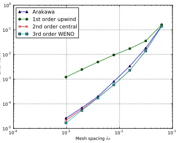
growth of numerical oscillations. When dissipation with H = 20 is included, the results are

shown in figure 3.

10-4 ₁₀-3 ₁₀-2 ₁₀-1

Mesh spacing δx

10-6 10-5 10-4 10-3 10-2 10-1 l

2 err

or

no

rm

Arakawa 1st order upwind 2nd order central 3rd order WENO

(a)l2 (RMS) error norm

10-4 ₁₀-3 ₁₀-2 ₁₀-1

Mesh spacing δx

10-5 10-4 10-3 10-2 10-1 100 l

∞ er

ror

no

rm

Arakawa 1st order upwind 2nd order central 3rd order WENO

(b)l∞

(maximum) error norm

FIG. 3. MMS test of advection operators. Equation 12 is solved on a 2D domain with

uniform grid spacing. The resolution varies from 16 × 16 to 1024 × 1024. Convergence

rates for second-order Arakawa (1.998), 1st_{-order upwind (0.993), 2}nd_{-order central}

differenc-ing (2.005), and 3rd-order WENO (2.019). All methods are limited to at best second-order

in mesh spacing δx due to the central differencing applied to φ and the boundary conditions.

Script:examples/MMS/advection/runtest

Both global error and local error are found to converge at the expected rate in the

asymptotic (small δx regime, as measured by the l2 _{(RMS) error in figure 3(a), and thel}∞

(maximum) error in figure 3(b) respectively. Apart from the first order upwind scheme, all

schemes converge at second order in grid spacing δx: The WENO scheme is formally third

order accurate in the bulk of the domain, but the advection velocity is calculated from φ

using 2nd_{-order central differences, and boundary conditions are only second-order accurate,}

reducing the overall convergence rate to second order. The WENO scheme implementation

cannot therefore be considered fully verified, and as noted above the verification of limiter

C. Schemes for wave equations

Along the magnetic field methods are implemented which model wave propagation, such

as sound and shear Alfv´en waves, and diffusion processes such as heat conductivity. Wave

propagation operators often appear in the form of coupled first order equations:

∂f

∂t =

∂g ∂x

∂g

∂t =

∂f

∂x (15)

The manufactured solution was chosen to be

f = 0.9 + 0.9x+ 0.2 cos(10t) sin(5x2)

g = 0.9 + 0.7x+ 0.2 cos(7t) sin(2x2)

and the equations are solved using staggered 2nd_{-order central differencing: Variable g was}

shifted to the cell boundaries, whilstf was cell centred. This arrangement requires different

handling of boundary conditions to account for this shift. To test boundary conditions and

handling of staggered variables, this test was performed in xand then iny(replacingxwith

y/2π in the above manufactured solutions).

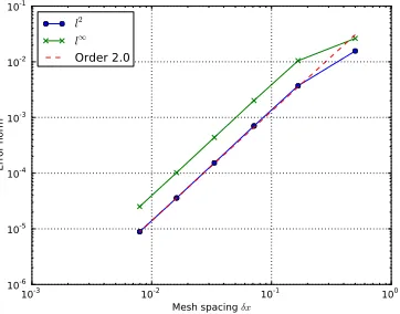
Results of a convergence test are shown in figure 4, which shows the l2 _{(RMS) and}

l∞ _{(maximum) error norms for quantity f as a function of the mesh spacing δx. This}

shows convergence at an order around 1.97, as expected for this scheme. This test has

been conducted with combinations of Dirichlet and Neumann boundary conditions, finding

essentially the same result in all cases.

10-3 ₁₀-2 ₁₀-1 ₁₀0

Mesh spacing δx

10-6 10-5 10-4 10-3 10-2 10-1

Error norm

l2

l∞

Order 2.0

FIG. 4. Error norms forf in wave equation 15 using 2nd_{-order central differencing. A convergence}

D. Second derivative operators

In order to verify the second derivative (diffusive) operators and boundary conditions,

a series of tests have been performed: First we verify the spatial convergence rate towards

a steady state (independent) manufactured solution; and then we verify using a

time-dependent manufactured solution.

1. Steady-state manufactured solution

In order to verify spatial convergence for time-dependent systems of equations, the

ap-proach taken in5 _{is to evolve the equations towards a steady-state solution. Here we use this}

approach to verify boundary conditions and second-order operators by solving the equation:

∂f

∂t =

∂2_f

∂x2 +S (16)

The manufactured solution is chosen to be

fM = 0.9 + 0.9x+ 0.2 sin 5x2

(17)

in the range 0 ≤ x ≤ 1 i.e. boundaries are at x = 0 and x = 1. The source function is

therefore:

S = 20x2sin 5x2

−2 cos 5x2

(18)

In contrast to the time-dependent MMS tests presented in this paper, for this steady-state

problem we initialise the simulation at t = 0 with f = 0, and not the exact manufactured

solution. This is suggested by5 _{since even though this increases the number of iterations}

to convergence, using the exact solution can hide coding mistakes. Equation 16 was then

integrated in time to t = 10 using an absolute tolerance of 10−15 _{and relative tolerance of}

10−7_{. This is a sufficiently long time that f reaches a steady state to within tolerances.}

Results are listed in table I, showingl2 _andl∞ _{errors and convergence rates. We first}

per-form the test with Dirichlet boundary conditions, then with mixed Dirichlet and Neumann

TABLE I. Error norms and convergence rates for integration of equation 19 as a function of number

of grid pointsN. Shown are cases with Dirichlet boundary conditions, then with one Dirichlet and

one Neumann boundary (mixed).

Dirichlet Mixed

N l2 Rate l∞ Rate l2 Rate l∞ Rate

8 2.624e-02 6.088e-02 3.504e-02 6.317e-02

16 4.332e-03 2.126 1.227e-02 1.890 5.514e-03 2.182 1.242e-02 1.919

32 9.224e-04 2.030 2.720e-03 1.978 1.165e-03 2.039 2.733e-03 1.986

64 2.149e-04 2.007 6.400e-04 1.993 2.712e-04 2.009 6.415e-04 1.997

128 5.199e-05 2.001 1.552e-04 1.997 6.554e-05 2.003 1.554e-04 1.999

256 1.271e-05 2.009 3.822e-05 1.999 1.607e-05 2.005 3.825e-05 2.000

512 3.395e-06 1.894 9.572e-06 1.986 4.000e-06 1.996 9.488e-06 2.000

2. Time-dependent manufactured solution

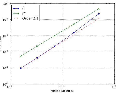
Diffusion equations in all three dimensions, separately and in combination, have been

verified, with convergence for one example shown in figure 5. The equation solved is

∂f

∂t =∇

2_{f (19)}

which is solved using 2nd_{-order central differences on a uniform grid. In 3D the}

manufacu-tured solution used was

f = 0.9 + 0.9x+ 0.2 cos (10t) sin 5x2−2z

+ cos (y) (20)

in the range 0 ≤ x ≤ 1; 0 ≤ y ≤ 2π and 0 ≤ z ≤ 2π. Results for a uniform 3D grid are

shown in figure 5, showing convergence at the expected order.

These tests confirm that these simple operators and the Dirichlet and Neumann boundary

conditions have been implemented correctly for uniform orthogonal grids. More complicated

geometries are tested in the next section, but the advantage of these simple tests is that

they run in under a minute on a desktop and so are now included in the standard BOUT++

10-2 ₁₀-1 ₁₀0

Mesh spacing δx

10-5

10-4

10-3

10-2

10-1

100

Error norm

l2 l∞ Order 2.1

FIG. 5. Error norms for diffusion equation 19 in 3D on a uniform grid as a function of grid spacing

δx, showing convergence with an order of 2.06. Script:examples/MMS/diffusion2/runtest

E. Coordinate systems

The field-aligned coordinate system used for tokamak simulations has been tested using

the analytic input mesh described in section III. The manufactured solution was

f = cos 4x4+ζ−θ

+ sin (t) sin (3x+ 2ζ−θ) (21)

wherex=ψ/∆ψis a normalised radial coordinate with a range between 0 and 1. The safety

factor was chosen to beq= 2 +x2_{, and inverse aspect ratioǫ= 0.1. Following the procedure}

outlined in section III, this results in toroidal and poloidal magnetic field components:

Bζ =

1

1−0.1 cos (θ) (22a)

Bθ =

0.1 (x2_{+ 2) [1−0.1 cos (θ)]}2

(1 + 0.1 cos (θ)) (22b)

and integrated shear

I = 1125x[θ+ 0.1 sin (θ)] (23)

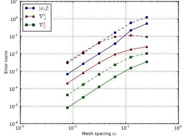
Results are shown in figure 6 for a range of resolutions from 43 _{to 128}3_{, showing}

con-vergence of the Arakawa bracket operator [φ, f], a perpendicular diffusion operator ∇2

⊥,

and parallel diffusion operator ∇2

||. Tests in both ballooning coordinates (equations 6,

to verifying these operators in non-orthogonal curvilinear coordinates, this test exercises the

twist-shift matching used to close field-lines in the core region of tokamak simulations, and

the calculation of radial derivatives in the shifted metric scheme. Note that in figures 6(a)

and 6(b) the parallel diffusion operator∇2

|| results are identical, as the use of shifted metrics

does not affect derivatives in the parallel direction (see section III).

10-3 ₁₀-2 ₁₀-1 ₁₀0

Mesh spacing δx

10-6 10-5 10-4 10-3 10-2 10-1 100 101 Error norm [φ,f] ∇2 ∇2 ||

(a)Ballooning coordinates. Convergence rates for

Arakawa bracket (2.03); perpendicular diffusion

operator (1.97); and parallel diffusion operator

(1.99)

10-3 ₁₀-2 ₁₀-1 ₁₀0

Mesh spacing δx

10-6 10-5 10-4 10-3 10-2 10-1 100 101 Error norm [φ,f] ∇2 ∇2 ||

(b)Shifted metric method. Convergence rates for

Arakawa bracket (2.07); perpendicular diffusion

operator (1.98); and parallel diffusion operator

(1.99)

FIG. 6. Verification of operators in toroidal field-aligned coordinates. Coordinate system and input

described in section III. Script:examples/MMS/tokamak/runtest

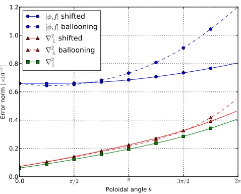
For this test case the reference poloidal angle θ0 in equation 10 was set to zero, so I = 0

atθ= 0. At θ= 0 thex−z mesh is therefore orthogonal, and there is no difference between

ballooning and shifted metric results in figure 7 at this location in θ. Moving away from

θ = 0 thex−z mesh becomes increasingly deformed, and differences between the ballooning

and shifted-metric procedures become apparent. As expected, the error norm is largest close

toθ = 2π where the mesh is most sheared, and the error at this point is reduced significantly

by using the shifted metric procedure. The shifted metric method is however not always

more accurate than the ballooning coordinate method, as shown for the advection operator

aroundθ =π/4 in figure 7, where the ballooning coordinates are more accurate: In general

the accuracy of these methods will depend on the solution. It has been found in simulations

of Edge Localised Modes with BOUT++30,31_{, that the use of the shifted metric method}

0.0 π/2 π 3π/2 2π

Poloidal angle θ

0.0 0.2 0.4 0.6 0.8 1.0 1.2

Err

or

no

rm

[×

10

−

3]

[φ,f] shifted [φ,f] ballooning

∇2 shifted ∇2 ballooning ∇2

||

FIG. 7. Comparison of RMS error norm for ballooning (dashed lines) and shifted-metric scheme

(solid lines), as function of poloidal angle θ, for the highest resolution case in figure 6 (1283 _grid

points). Integrated shear I (equation 10) is zero atθ= 0, and a maximum atθ= 2π.

abruptly. This coordinate system is used in section V B to verify the 3-field equations used

for ELM simulations.

F. Flux Coordinate Independent scheme

To verify the interpolation and central differencing schemes implemented in BOUT++

for FCI coordinates, we simulate a wave (equation 15) in a sheared slab. On each x−z

plane perpendicular to the magnetic field a Cartesian mesh is used, and the magnetic field

is sheared so that the points to be interpolated (small open circles in figure 1) span a range

of locations between neighbouring grid points.

A sheared slab of size Ly = 10m along the magnetic field; Lx = 0.1m in the

ra-dial direction, and Lz = 1m in the binormal direction was used, with magnetic field

(Bx, By, Bz) = (0,1,0.05 + (x−0.05)/10). The variation of the magnetic field-line pitch

with x therefore ensures that the interpolation location varies so as to test the 3rd_-order

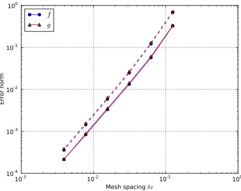
Hermite interpolation scheme. The manufactured solution used was

f = sin (y−z) + cos (t) sin (y−2z) (24a)

whereyand z are normalised to be between 0 and 2π in the domain (as in all manufactured

solutions presented here).

10-3 ₁₀-2 ₁₀-1 ₁₀0

Mesh spacing δx

10-4

10-3

10-2

10-1

100

Error norm

f g

FIG. 8. Convergence of f (1.95) and g (2.04) in equation 15 solved using the FCI method in

a sheared slab. Solid lines show l2 (RMS) error, whilst dashed lines show l∞ (maximum) error.

Script:examples/fci-slab/runtest

Figure 8 shows the error norm as the resolution in both parallel and perpendicular

direc-tions is varied. This shows second-order convergence, most likely limited by the accuracy of

the second-order central differencing scheme used to calculate parallel derivatives. Note that

in order to obtain good convergence, it was necessary to stabilise the collocated scheme, by

adding a parallel diffusion term of the formδx2_∂2

|| to each equation. This has been previously

discussed in the context of MMS testing of collocated numerical schemes in5_.

V. MODELS

After verification of individual operators, the MMS technique is now applied to the

ver-ification of entire models, which combine operators and couple multiple fields. Here three

models of interest are verified: the 2-field Hasegawa-Wakatani system (section V A), a

3-field reduced MHD model which has been used extensively to simulate Edge Localised Modes

(ELMs) with BOUT++ (section V B), and a 5-field cold-ion model for tokamak edge

Due to the large number of models which have been implemented in BOUT++, we have

introduced a naming scheme which can be used in future publications to refer to a specific

model. A scheme BOUT++/name/year such as BOUT++/HW/2014 is used here.

A. Hasegawa-Wakatani (BOUT++/HW/2014)

The Hasegawa-Wakatani model is a good starting place as it contains many of the

ele-ments of more complicated models, such as Poisson brackets, diffusion, and calculation of

electrostatic potential from vorticity, whilst being 2-D and faster to run than 3D models

at high resolutions. As such, it often forms a starting point for the construction of more

complex models. The equations solved are for plasma density n and vorticityω =~b0· ∇ ×~v

where~v is the E×B drift velocity in a constant magnetic field, and~b0 is the unit vector in

the direction of the equilibrium magnetic field:

∂n

∂t =−[φ, n] +α(φ−n)−κ ∂φ

∂z +Dn∇

2

⊥n (25a)

∂ω

∂t =−[φ, ω] +α(φ−n) +Dω∇

2

⊥ω (25b)

∇2_⊥φ=ω (25c)

The manufactured solutions were chosen to be

n = 0.9 + 0.9x+ 0.2 cos (10t) sin 5x2−2z

(26a)

ω = 0.9 + 0.7x+ 0.2 cos (7t) sin 2x2−3z

(26b)

φ = sin (πx)

0.5x−cos (7t) sin 3x2−3z

(26c)

along with parameters

α = 1 κ= 1

2 Dn= 1 Dω = 1 (27)

These parameters were chosen so that the magnitude of each term in equations 25 was

comparable; in a realistic simulation the parameters might be different, in particular the

diffusion terms Dn,ω would generally be smaller than is used here. This does not present

a problem for verification, since the correctness of the numerical method implementation

does not depend on these parameters. If the code is correct with Dn = 1 then it will

with arbitrary parameters, and in general the required resolutions and stability critera (e.g.

maximum timestep) will be problem specific.

Note that the solution for both vorticity ω and potentialφare manufactured, despite the

two quantities being related through the vorticity equation 25c. This avoids integration of

manufactured solutions, and is handled by adding an analytic source term to the right hand

side of equation 25c.

Results are shown in figure 9, calculated on a 2D unit domain, showing the l2 _{and l}∞

norms over bothn and ω, and a fit showing second order convergence. This shows that the

10-3 ₁₀-2 ₁₀-1

Mesh spacing δx

10-5

10-4

10-3

10-2

10-1

Error norm

l2 l∞ Order 2.0

FIG. 9. Error norm of Hasegawa-Wakatani system (n and φ, equations 25) on a Cartesian

mesh, showing second-order convergence. Mesh resolutions range from 16× 16 to 512×512.

Script:examples/MMS/hw/runtest

operators in equation 25 including the inversion of potentialφ from vorticityω are correctly

implemented, at least on orthogonal uniform grids. We now proceed to test these operators

in toroidal field-aligned coordinate systems typical of realistic BOUT++ simulations.

B. 3-field reduced MHD (BOUT++/FLUID3/2014)

The 3-field model used for ELM simulations1,30,31_{has been verified in field-aligned toroidal}

geometry with a radially varying safety factor q, using the shifted metric coordinate system

implemented in BOUT++ in coordinate systems with a non-trivial metric tensor.

The equations evolved are for vorticity ω = ~b0 · ∇ × ~v, pressure p, and the parallel

component of the magnetic vector potential A|| =~b0 ·A, where~ ~b0 = ~ B0

|_B~0|;

~

B0 is the unit

vector along the equilibrium magnetic field B~0, and B0 = ~ B0

is the magnitude of the

magnetic field

ρ0

dω

dt =B

2 0∂||

J||

B0

+ 2~b0×~κ0· ∇p (28a)

∂A||

∂t =−∂||φ−ηJ|| (28b)

dp

dt =−

1 B0

~b0× ∇φ· ∇p0 (28c)

ω = 1

B0

∇2_⊥φ (28d)

J|| =J||0−

1 µ0

∇2_⊥A|| (28e)

where the parallel derivative includes the perturbed magnetic field:

∂|| =~b0· ∇ −

1 B0

~b0× ∇A||· ∇ (29)

where ’0’ subscripts denote equilibrium (starting) quantities: ρ0 is the (constant) density;

~

B0 the magnetic field;κ0 =

~b0· ∇

~b is the field-line curvature. The electrostatic potential φ is calculated from the vorticity by inverting a perpendicular Laplacian (with Dirichlet

boundary conditions here), and the parallel current J||=~b0·J~is calculated from the vector

potential. The convective derivative is defined as

d dt = ∂ ∂t+ 1 B0

~b0× ∇φ· ∇ (30)

Background (equilibrium) profiles are chosen to mimic realistic cases, with a pedestal-like

pressure profileP0, and a parallel current profileJ0which peaks on the outboard and inboard

midplanes:

P0/P = 2 + cos (πx) J0/J = 1−x+ sin2(πx) cos (θ) (31)

wherexis the normalised radial coordinate, which lies between 0 and 1, andθ is the poloidal

angle, which lies between 0 and 2π. Normalisation parameters are

ne= 1019 m−3 Te= 3 eV L= 1m B = 1T (32)

The manufactured solutions used were:

φ=

sin (z−x+t) + 10−3cos (y−z)

sin (2πx) (33a)

ψ = 10−4cos 4x2+z−y

(33b)

U = 2 sin (2t) cos (x−z+ 4y) (33c)

P = 1 + 1

2cos (t) cos 3x

2 _−2z

+ 5×10−3sin (y−z) sin (t) (33d)

A Lundquist number of S = 10 was used to set the resistivity η. This is so that the

resistive term in Ohm’s law (equation 28b) becomes comparable to the other terms, and

S is much smaller (higher η) than would be the case in a realistic tokamak simulation, for

which S = 108 _{would be more typical.}

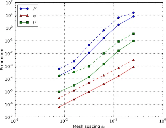
Results are shown in figure 10, with the l2 _{and l}∞ _{norms shown for each evolving}

vari-able (P, ψ, U). The slow convergence at large mesh spacing (small resolution) is due to the

10-3 ₁₀-2 ₁₀-1 ₁₀0 Mesh spacing δx

10-7 10-6 10-5 10-4 10-3 10-2 10-1 100 101 102

Error norm

P ψ U

FIG. 10. Error norms for 3-field set of equations. Solid lines show the l2 (RMS) error norms,

whilst dashed lines are the l∞ (maximum) error. Convergence orders for pressure p is 1.95;

vorticity ω is 1.64; and vector potential A_|| is 2.01. Resolutions range from 43 to 1283.

Sc-tript:examples/MMS/elm-pb/runtest

solutions being under-resolved: the smallest grids have only 4 grid points in each dimension,

insufficient to resolve the manufactured solution. At high resolution the pressure and

at a rate between first and second order. The maximum (l∞_{) error in vorticity converges}

at close to 1st _{order at high resolution, indicating that the source of this slow convergence}

is an order 1 error on a sub-set of the domain, so that when averaged over the domain the

RMS (l2_{) error converges at a faster rate than the maximum error. The location of the error}

maximum at high resolution is at the radial boundary, but the reason for this is not yet clear

despite extensive investigation. Here we conclude that although the model does converge,

it does not converge at the expected rate, and further investigation is needed.

C. BOUT++/FLUID5/2014

Finally, the set of equations implemented in the Global Braginskii Solver (GBS) code32

have been implemented in BOUT++ and verified in a simplified form using the Method of

Manufactured Solutions. In this current work electromagnetic effects and ion viscosity terms

ω, Ohm’s law, and parallel ion velocityV||i:

∂n

∂t =−

R ρs0

1

B [φ, n] + 2n

B

C(Te) +

T

nC(n)−C(φ)

−n~b· ∇V||e−V||e

~b· ∇n+D(n) +S (34a)

∂Te

∂t =−

R ρs0

1

B [φ, Te]−V||e

~b· ∇Te

+4 3 Te B 7

2C(Te) + Te

n C(n)−C(φ)

+2Te 3

"

0.71~b· ∇V||i−1.71

~b· ∇V||e

+0.71 V||i−V||e

n

~b· ∇n

#

+DTe(Te) +D

||

Te(Te) +ST (34b)

∂ω

∂t =−

R ρs0

1

B [φ, ω]−V||i

~b· ∇ω

+B2

"

~b· ∇ V||i−V||e

+ V||i −V||e

n

~b· ∇n

#

+2B

C(Te) +

Te

nC(n)

+Dω(ω) (34c)

∂V||e

∂t =−

R ρs0

1 B

φ, V||e

−V||e

~b· ∇V||e

− mi

me

ν V||e−V||i

+ mi me

~b· ∇φ

− miTe

nme

~b· ∇n−1.71mi me

~b· ∇Te+DV||e V||e

(34d)

∂V||i

∂t =−

R ρs0

1 B

φ, V||i

−V||i

~b· ∇V||i

−~b· ∇Te+

Te

n

~b· ∇n+DV_||i V||i

(34e)

where

ρs0 =

Cs0

Ωci

Cs0 = s

eTe

mi

Ωci=

eB mi

(35)

with vorticity and the curvature operator defined as

ω =∇2_⊥φ C(A) = B

2 ∇ ×

~b B

!

Here the dissipation operators D(·) were hyper-diffusion terms in the plane perpendicular

to the magnetic field of the form:

D(f) =−δx4∂

4_f

∂x4 −δz 4∂4f

∂z4 (37)

In order to test all terms in this set of equations, the parameters of the simulation should

be chosen so that the magnitude of each term is of a similar order of magnitude. If this is

not done, then the error in the result will be dominated by a small number of operators,

and mistakes in the implementation of small terms may not become apparent until very

high (possibly impractical) resolution is reached. In order to handle the large number of

terms in equations 34a-34e, the magnitude of each term was estimated using SymPy by

replacing trigonometric functions sin (·) and cos (·) by their maximum value (1), and the

coordinates (x, θ, ζ) by their maximum values (1,2π,2π). This allowed parameters to be

quickly adjusted to find useful regimes. The resulting manufactured solutions are:

n= 0.9 + 0.9x+ 0.5 cos (t) sin 5x2−z

+ 0.01∗sin (y−z) (38a)

Te = 1 + 0.5 cos (t) cos 3x2 −2z

+ 0.005 sin (y−z) sin (t) (38b)

ω = 2 sin (2t) cos (x−z+ 4y) (38c)

Ve = cos (1.5t)

2 sin (x−0.5)2+z

+ 0.05 cos 3x2_+y−z

(38d)

Vi =−0.01 cos (7t) cos 3x2+ 2y−2z

(38e)

φ= [sin (z−x+t) + 0.001 cos (y−z)] sin (2πx) (38f)

Parameters used were:

Te= 3eV ne = 1019m−3 B = 0.1T mi = 0.1mp (39)

wheremp is the mass of the proton. Light ions were used in order to reduce the difference in

timescales between electrons and ion dynamics. Note that the manufactured solutions and

parameters are not required to be realistic, provided that they do not violate any constraints

such as positivity of density and temperature, as discussed in section II.

Simulations were performed in a 3D slab geometry, with resulting error norms shown in

figure 11. In this geometry the curvature polarisation vector ∇ × _B~b is set to a constant in

the z (binormal) direction. All fields show convergence at the expected rate, approximately

2nd_{-order in mesh spacingδx. This demonstrates that complex models can be verified using}

10-3 ₁₀-2 ₁₀-1 ₁₀0 Mesh spacing δx

10-6 10-5 10-4 10-3 10-2 10-1 100

Error norm

Ne

Te

Vort

VePsi

Vi

FIG. 11. Error norms for 5-field set of equations. Solid lines show thel2(RMS) error norms, whilst

dashed lines are the l∞ (maximum) error. Convergence orders for density Ne is 2.02; electron

temperatue Te is 2.70; Vorticity ω is 2.04; Electron parallel velocity Ve is 2.36; and ion velocityVi

is 2.42. Resolutions range from 83 to 1283. Script:examples/MMS/GBS/runtest-slab3d

VI. CONCLUSIONS AND DISCUSSION

The Method of Manufactured solutions has been used to rigorously test numerical

meth-ods implemented in BOUT++, both independently as unit tests, and in combination as

simulation models. Convergence to the correct solution at an asymptotic 2nd _{order has been}

demonstrated for large sub-sets of the BOUT++ framework: Though higher order methods

(3rd_{-order WENO and 4}th_{-order central differencing) are implemented in BOUT++, the}

overall convergence rate is limited to 2nd _{order by the boundary conditions.}

Mechanisms have been implemented into BOUT++, which simplify and partly automate

the process of verifying the correctness of a numerical implementation, requiring minimal

modifications to the code between production simulations and verification runs. This will

facilitate the routine use of the MMS as an increasing variety of models are implemented

in BOUT++. Since code verification is an ongoing process, particularly for an actively

developed scientific code such as BOUT++, the methods and tests detailed here are now

used as part of a test suite which is run routinely and automatically (using Travis-CI) to

It is important to note the limitations of the present work, which will be the subject

of further development. Whilst curvilinear coordinates in tokamak geometry with varying

safety factor have been verified, no tests have yet been performed in X-point geometry.

The Flux Coordinate Independent (FCI) scheme has been implemented in BOUT++, but

only tested in sheared slab geometry. Investigation of methods for simulations of X-point

geometry, including FCI, and verification with MMS will be the subject of future work.

ACKNOWLEDGMENTS

This work has been carried out within the framework of the EUROfusion Consortium

and has received funding from the Euratom research and training programme 2014-2018

under grant agreement No 633053. The views and opinions expressed herein do not

nec-essarily reflect those of the European Commission. The authors gratefully acknowledge

the support of the UK Engineering and Physical Sciences Research Council (EPSRC)

un-der grant EP/K006940/1, and Archer computing resources unun-der Plasma HEC consortium

grant EP/L000237/1.

REFERENCES

1_{B D Dudson, M V Umansky, X Q Xu, P B Snyder, and H R Wilson. Comp. Phys. Comm.,}

180:1467–1480, 2009.

2_{B D Dudson, A Allen, G Breyiannis, E Brugger, J Buchanan, L Easy, S Farley,}

I Joseph, M Kim, A D McGannn, J T Omotani, and M V Umansky. J. Plasma Phys.,

81(01):365810104, 2015. doi:10.1017/S0022377814000816.

3_{P J Roache. Verification and Validation in Computational Science and Engineering.}

Her-mosa Publishers, Albuquerque NM, 1998.

4_{W L Oberkampf and C J Roy. Verification and Validation in Scientific Computing.}

Cam-bridge University Press, New York, NY, USA, 2010.

5_{K Salari and P Knupp. Code verification by the method of manufactured solutions.}

Tech-nical Report SAND2000-1444, Sandia National Laboratories, 2000.

6_{M V Umansky, R H Cohen, L L LoDestro, and X Q Xu. Contrib. Plasma Phys.,}

7_{C J Roy, C C Nelson, T M Smith, and C C Ober. Int. J. Num. Methods in Fluids,}

44(6):599–620, 2004.

8_{D Kalupin, V Basiuk, D Coster, Ph Huynh, L L Alves, Th Aniel, J F Artaud, J P S}

Bizarro, C Boulbe, R Coelho, D Farina, B Faugeras, J Ferreira, A Figueiredo, L Figini,

K Gal, L Garzotti, F Imbeaux, I Ivanova-Stanik, T Jonsson, C J Konz, E Nardon, S Nowak,

G Pereverzev, O Sauter, B Scott, M Schneider, R Stankiewicz, P Strand, I Voitsekhovitch,

ITM-TF contributors, and JET-EFDA Contributors. InEurophysics Conference Abstracts

(Proc. of the 35th EPS Conference on Plasma Physics, Hersonissos, Crete, 2008), volume

32D, pages P–5.027, 2008.

9_{C S Chang, S Ku, P Diamond, M Adams, R Barreto, Y Chen, J Cummings, E D’Azevedo,}

G Dif-Pradalier, S Ethier, L Greengard, T S Hahm, F Hinton, D Keyes, S Klasky, Z Lin,

J Lofstead, G Park, S Parker, N Podhorszki, K Schwan, A Shoshani, D Silver, M Wolf,

P Worley, H Weitzner, E Yoon, and D Zorin. J. Phys.: Conf. Ser., 180:012057, 2009.

10_{F Riva, P Ricci, F D Halpern, S Jolliet, J Loizu, and A Mosetto. Physics of Plasmas,}

21:062301, 2014.

11_{C Michoski, D Meyerson, T Isaac, and F Waelbroeck. Discontinuous galerkin methods for}

plasma physics in the scrape-off layer of tokamaks. J. Comput. Phys., 274:898–919, 2014.

12_{SymPy Development Team. SymPy: Python library for symbolic mathematics, 2014.}

13_{R LeVeque. Finite Difference Methods for Ordinary and Partial Differential Equations.}

SIAM, 2007.

14_{W D Haeseler. Flux Coordinates and Magnetic Field Structure. Springer, 1991.}

15_{X Q Xu, M V Umansky, B Dudson, and P B Snyder. Boundary plasma turbulence}

simulations for tokamaks. Comm. in Comput. Phys., 4(5):pp. 949–979, November 2008.

16_{A M Dimits. Phys. Rev. E, 48(5):4070–4079, Nov 1993.}

17_{B Scott. Physics of Plasmas, 8(2):447, 2001.}

18_{F Hariri and M Ottaviani. Comp. Phys. Comm., 184(11):2419–2429, 2013.}

19_{A Stegmeir, D Coster, O Maj, and K Lackner. Contrib. Plasma Phys., 54:549–554, 2014.}

20_{Areih Iserles. A First Course in the Numerical Analysis of Differential Equations.}

Cam-bridge University Press, 2009. ISBN: 978-0-521-73490-5.

21_{G E Karniadakis, M Israeli, and S A Orszag. J. Comput. Phys., 97:414, 1991.}

22_{B D Scott. GEM - an energy conserving electromagnetic gyrofluid model. arXiv:physics,}

23_{S Gottlieb, C-W Shu, and E Tadmor. SIAM Review, 43(1):89–112, 2001.}

24_{A C Hindmarsh, P N Brown, K E Grant, S L Lee, R Serban, D E Shumaker, and C S}

Woodward. SUNDIALS: Suite of nonlinear and differential/algebraic equation solvers.

ACM Transactions on Mathematical Software, 31(3):363–396, 2005.

25_{Satish Balay, William D. Gropp, Lois Curfman McInnes, and Barry F. Smith. In E. Arge,}

A. M. Bruaset, and H. P. Langtangen, editors, Modern Software Tools in Scientific

Com-puting, pages 163–202. Birkhauser Press, 1997.

26_{S Balay, S Abhyankar, M Adams, J Brown, P Brune, K Buschelman, V Eijkhout, W Gropp,}

D Kaushik, M Knepley, L Curfman McInnes, K Rupp, B Smith, and H Zhang. Technical

Report ANL-95/11 - Revision 3.5, Argonne National Laboratory, 2015.

27_{Arakawa. A. J. Comput. Phys., 1:119–143, 1960.}

28_{Guang-Shan Jiang and Chi-Wang Shu. J. Comput. Phys., 126:202–228, 1996.}

29_{Guang-Shan Jiang and Danping Peng. SIAM J. Sci. Comp., 21(6):2126–2143, 2000.}

30_{X Q Xu, B Dudson, P B Snyder, M V Umansky, and H Wilson. Phys. Rev. Lett.,}

105:175005, 2010.

31_{B D Dudson, X Q Xu, M V Umansky, H R Wilson, and P B Snyder. Plasma Phys. Control.}

Fusion, 53:054005, 2011. doi: 10.1088/0741-3335/53/5/054005.

32_{P Ricci, F D Halpern, S Jolliet, J Loizu, A Mosetto, A Fasoli, I Furno, and C Theiler.}