Optical and digital methods for the analysis of microscopic tissue sections

OPTICAL AND DIGITAL METHODS

FOR THE ANALYSIS OF

MICROSCOPIC TISSUE SECTIONS

by

A.R.Eastgate, B.Eng., M.Sc.(Qual)

Submitted in partial fulfilment

of the requirements for the degree

of Master of Science.

or diploma in any university, and that, to the best of my knowledge and belief, this thesis contains no copy or paraphrase of material previously published or written by any other person, except where due reference is made in the text of the thesis.

( A.R.Eastgate )

CONTENTS

ABSTRACT

Page

CHAPTER

1.

Introduction

1

2.

Scanning Microphotometry 3

Blur and Aliasing

6

Signal to Noise Ratio 10

3.

Digitisation of Static TV Images 11

Measuring Requirements . 14

Hardware Details

16

4.

Quantitation Using the Laplacian Operator 18

The Gradient Operator 20

5.

Texture Analysis of Tissue Sections 22

Prostate Tissue Scanning' 25

Feature-Space Diagrams

30

6.

Micro-spectrophotometry - 32

The Optica CF4 Monochromator 34

7.

Conclusion

38

Appendix 1 :

Television Digitisation Programs

41

Appendix 2 :

Image-Analysis Programs

45

Appendix 3 :

Program 'SPAA'

50

This thesis presents optical and

computer-based methods for the analysis of microscope specimens

that are in the form of thin sections that have been

mounted on standard glass slides.

Three methods are discussed whereby image

and photometric information can be obtained -

television scanning, microphotometric scanning and

micro-spectrophotometry. The limitations of these

methods are analysed and some representative results

are given.

The thresholding of digital image data with

the assistance of neighbourhood operators is examined,

with particular reference to the Laplacian and Gradient

operators.

A method for the statistical analysis of

tissue-section textures is presented and is shown to

be applicable the discrimination of two pathological

classes of human prostate tissue. The effectiveness

of the method is evaluated by the use of a computed

1

Chapter 1 : Introduction

The task of image analysis is one that pervades our daily lives so thoroughly that we are scarcely, if ever, aware of the range and sophis-tication of the intellectual processes constantly at work behind those obvious witnesses to our visual activity, the eyes. Decisions about colour, texture, shape and spatial disposition are continually being made in only fractions of seconds, with the least conscious direction required; it is all, as we say, automatic.

In terms of that quantum of the information world, the bit, the number of quanta required to fully describe a typical outdoor scene down to the resolution of the human eye is almost astronomical. Billions of constantly-changing bits would be required for such a scene. The first task of visual perception is to determine what is relevant and to reduce this information surplus to manageable levels.

In the detection and recording of microscopic detail, which is the subject of the first parts of this study, reduction of the information in the image of the specimen will be shown to be an inevitable consequence of the nature of the sampling processes used : scanning microphotometry and television scanning. The nature of this information-loss is discussed.

With many microscope specimens the final result of the analysis can be expressed in surprisingly few words. Often it is only a proportion that is sought, such as "13.4% Diopside", for the geologist, or a choice between two alternatives, such as a Cancer/Benign diagnosis for the clinician.

Even more surprising is the extent of the information about

automata to "understand" a scene, something which is still being actively researched. Hall (1.1) gives a summary of what has been achieved in this field; he divides scene comprehension into four tasks: segmentation, region-description, relational description and object formation.

Segmentation requires an understanding of spatial relationships in the general case, as does the formation of relational descriptions such as "behind" or "inside of". The region-description task for the case of two-dimensional microscope images and the derivation of sensible

conclusions about these images , the object formation task, is shown to be achievable with a microcomputer.

-3

Chapter 2 Scanning Microphotometry

A microphotometer can form scanned images of microscope specimens when the microscope stage is motor-driven and can translate the specimens under the objective lens in a programmed pattern. The images thus formed are slow to collect but usually have a high signal to noise ratio. The primary requirement in such scanning may often be the collection of stat-istical information about inhomogeneous specimens, in which case image fidelity may be sacrificed for an increase in speed. Sandritter and Kiefer

(2.1) give a comprehensive review of microphotometer instrumentation and methodology, as does Zimmer (2.2); only the advent of the powerful and inexpensive range of modern microcomputers in the last decade requires a deeper investigation of the microphotometer's potential, particularly in the area of digital image acquisition and analysis.

The Leitz MPV2 microphotometer has two motorized stepping-stages, with 0.5 m and 10 m. step sizes. An interface between the MPV2 and its instrument-computer, an Acorn BBC Micro, has been constructed by the author to match the computer's parallel-port TTL-level signals to the inputs of the stepping-stage drive circuitry and to match the output of the MPV2 photometer-amplifier to the input of the computer's analogue-to-digital converter (ADC). Thus there are two restrictions upon scanning speed : the minimum conversion-time of the ADC is 4 milliseconds and the minimum time required for each step of the motorized stage is approximately the same. Allowing a 2 millisecond 'overhead' per sample-point for direction-changes and other system delays, the minimum time for a typical scan of 16,384 points is just under three minutes; experience has shown this to be an acceptable figure for most applications to date.

Obtaining image-fidelity is mainly a matter of keeping illumination as strong as possible and ensuring that the stepping-stage does not stall

cleanliness, the luminous-field and measuring stops should be carefully adjusted for relative size and concentricity, and the instrument must be free of zero-error (due to dark current, for example) and drift. Under the best possible conditions a sample as small as 10,000 molecules should be able to be detected (2.2). A comprehensive description of the microphotometer and its method of operation has been given in an earlier report (2.3).

The theory of scanned image formation has been extended greatly since Mertz and Gray published their pioneering paper on television images in 1934 (2.4). Fourier analysis of the sampling process has shown that a two-dimensional sampling of a band-limited image f(x,y) can completely represent the image if samples are taken with separations no greater than

1 1

Zix = -Irr- and Ily = 2-07 , where W u and W v are the spatial frequency cwu

limits of the image in the x and y directions (2.5).

In the scanning microphotometer the light-sampling is performed by a sampling-aperture of finite size and is markedly affected by diffraction for diameters less than one micron. Usually the aperture is square or circul-ar and ranges in diameter from 0.5pm. to 100pm. In analysis of this sampling the filtering effect of the aperture can be described by its point-spread function ( PSF ), h(x,y). The spatial frequency limits in the original image are generally those imposed by the microscope optics and are at least an order of magnitude beyond the representation limits imposed by Shannon's sampling theorem above (-.20/pm.) when the usual ( 10Fm.) stepping-stage is in operation. Thus the choice of sampling-aperture size must be made mainly with regard to the size of the step between samples and the need to make a compromise between adequate light throughput to the photometer and the avoidance of blur (when the sampling-aperture diameter is too large).

5

= One-dimensional Edge

Unit Dislocation

F = 0

-2 -1

x=0

XU 1 2

as

error =

jXk

=

t

if

is

,

For

s

0 otherwise

Scanning-Aperture Characteristic

X = 0

s

(x— u)

(Continuous) Scanned Result

[image:9.558.48.489.77.432.2]

1 X: U

Figure 2-1 : Scanning Over An Idealised Dislocation.

instantaneous field of view ( IFOV ) in units of sample interval, then the resulting scanned image is a ramp of width s and is centred at x=u, the convolution of h(x) and f(x-u) :

g(x-u) = h(x)-* f(x-u)

1 for x ). Eu + (s/ 2)1 x-u +- _{for Ix-u14}

s/2 s

2

0 for x<:[u -(s/2)]

Thus the error resulting from such a sampling can be calculated (error)2 = fjf(x-u)-g(x-4dx

s

=

.fu+,/2

_s

f(x-u)-(---- ).x-u 2 dx s

2 2

= r

u(

1:1

)

_{dx +}

1

)

_{1 (x-u) dx}

J

s

s

s

11.-.

51 12

diffraction effects and when the sampling intervals are very small, the sampling aperture should be kept as small as possible. Light throughput is always a limiting factor however and aberrations in the objective lens are thought to modify the PSF of the system slightly. Aberration has been modelled by Goodman (2.6) as a phase-shifting plate inserted in the aperture and whose sole effect is to produce phase distortions within the pass-band of the system. The effect of diffraction for the normal range of aperture-sizes can be seen to be quite small from the relationship plotted in Fig.2-2 below. Deviation from linearity in these plots is more due to inaccuracy in manual setting of the aperture-size than anything else.

A general analysis of image degradation due to aliasing and blur in discrete data obtained with optical scanners has been presented by Huck et al.,(2.7). The optimisation of shape for apertures of constant transmitt-ance has been dealt with by Katzberg et al.(2.8) and it was shown that a diamond-shaped aperture combined with an electronic low-pass filter reduces aliasing to the levels obtained with a graded-transmittance (Gaussian)

aperture. The square and circular apertures used in the MPV2 microphotometer are thus inferior in this respect; their spatial-frequency responses have significant side-lobes, so that the resulting admission of high spatial frequency image content is best reduced by decreasing the sampling intervals or increasing aperture diameters. An analysis of this problem follows.

If we denote the effective aperture-width by

y

and the sample-steps in the two orthogonal directions by X and V. then the sample-intervals can be expressed as sx= X/Is and sy= Y/2f . Normally sx=sy for the micro-photometer scanning process, and X = Y = 101km. For most image-scanning systems 0.5s4;1.0 and there is still controversy as to which value of s is generally 'best'. Huck et al. (2.7) computed the relative amounts of blur and aliasing produced by a circular aperture of constant transmittance (and

Illumination Current: 4.80 A. Objective Power: X25 7

0 10 20 30 40 50 60

70

Diameter of Measuring Aperture

(pm.)

Fig.2-2: Relationship between Photometer Signal

at the scanned image formation of a random field of two-dimensional pulses whose widths r obey a Poisson probability density function with expected mean width

p r

and whose magnitudes obey a Gaussian probability density function with variance 012 . The Wiener spectrum of such a field is :

2.TE /42 OZ2 2

Clo W ) , where /0= V2 +W 2

1+(27r/y and its autocorrelation function is :

y2 .

95 ( r ) = CT. exp( 2 -r ) , where r2 . x 2 4. iur

This random field is similar to a wide range of scenes, including well-focussed microscope images of natural tissue sections. A sensor, the PMT with its sampling aperture in the case of the microphotometer, converts this continuous random field L(x,y) into the sampled form s(x,y;X,Y) that is stored in the memory of the instrument computer as discrete values. Thus the processes to be analysed are described by the equations :

s(x,y) = L(x,y)* h(x,y) , a convolution, and s(x,y;X,Y) = s(x,y).comb( , ) .

The Fourier transform of the sampling equation above can be otherwise

O 00 A

expressed as : Is'(v,w;X,Y) =E

T,L

08,—;,1 )

mr--oo —NJ ,s I

A

= A S(V,W) + Sa(V,YV ;X,Y) ,

A A

where

(v,w)

is the continuous (unsampled) component and s a (V,v);X,Y)

represents the sideband components generated by sampling. Halyo and Stallman (2.9) have shown that the spectral components in the reconstructed signal r(x,y) due to i (),,I,o) and /01 (v,w;X,Y) are statistically independent and stationary processes if the continuous random field L(x,y) is a real, Gaussian process. Thus the aliasing component r a (x,y) can be treated as an additive noise. The Wiener spectrum of the reconstruction can be expressed

A A A

100

_

••■••■•

-2 1

0 •5

9

the pass-band of the reconstruction process and can be expressed as :

A 00 °0 A _A

m -too 0(Y- W - _Y t) _SX

(

0,_1-72,W_L)

21tcr

- (y a

A 0)

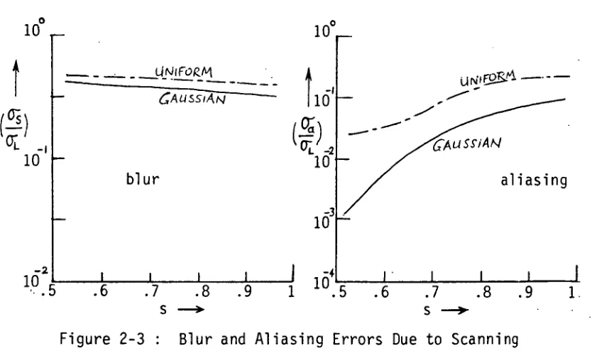
where T5 and Ta are the spatial frequency responses of the sampling and reconstruction processes respectively. Thus the blur and aliasing errors introduced when a random field of the type described above is scanned can be calculated. The errors computed by Huck et al.(2.7) for the sampling range 0.5s‘1.0 were the evaluation of the following integrals

for blur : us .J_{T$1( 1/, 14,} . _{)dv.dw , and} _w

for aliasing : 2

j

'

7

(von/ )dv.dw

The variance of the input signal, the random field, is given by : DO

, 2

rr

O7

_L

₌

_jj

,W )dv.dw . -co

Plots of these blur and aliasing errors, taken from Huck et al.(2.7) for a random field with (Ph) --(1/3) scanned with a circular aperture and two types of transmittance profile ( one uniform and the other Gaussian ),are given below by Fig.2-3 .

10°,-

_ UNIFoktvl

CAussrAN

1'

₁₆

₄

U r,.-2S-t P1

CAuSSVAN

10

blur aliasing

1 I I I

I

1

64 1 I I 1

.6 .7 .8 .9 I .5 .6 .7 .8 .9 1

[image:13.555.59.476.484.731.2]

S —> S

It can be seen from Fig.2-3 above that there is a distinct gain in image quality to be had by allowing overlap to occur in scanning systems, even up to the level of s = 0.5, regardless of the transmittance profile of the scanning aperture. There is further improvement in grading the transmittance profile in a form close to Gaussian; this should be possible to do photographically with regular microphotometer apertures, since their minimum diameters are usually of the order of 500/m, much greater than typical emulsion grain sizes.

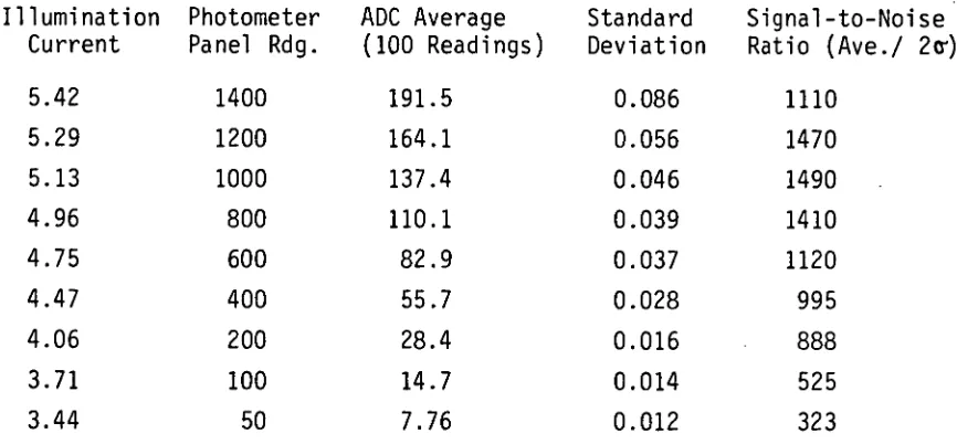
The signal-to-noise ratio ( SNR ) of the combined MPV2 micro-photometer and instrument-computer ADC was measured at various levels of illumination, using the normal settings of PMT-voltage and sampling-aperture diameter that are employed in scanning with the lOpm. stepping stage : V pmt = 600 Volts, D sa = 1211m. As has been mentioned above, the SNR values are quite high; the SNR is also best when the illumination is high. See Table 2.1 below :

Illumination Current

Photometer ADC Average Standard Signal-to-Noise Panel Rdg. (100 Readings) Deviation Ratio (Ave.! 2v)

5.42 1400 191.5 0.086 1110

5.29 1200 164.1 0.056 1470

5.13 1000 137.4 0.046 1490

4.96 800 110.1 0.039 1410

4.75 600 82.9 0.037 1120

4.47 400 55.7 0.028 995

4.06 200 28.4 0.016 888

3.71 100 14.7 0.014 525

[image:14.556.69.502.442.643.2]

3.44 50 7.76 0.012 323

25%

BLACK LEVEL

LINE

INTERVAL

64-.21us.

BACK Pokcil

HORiZoNTAL SYNC. PaLsE5

5,4s.t 5% / 2/is. 5%

FRoNT poRcAl

MERTicAI-S

INTWAL _,1

EeDUAL/sw; Pu4sES

r‹—

%

H

I

L

cll

i

I 1 I

I

1

1

1

1

I

END

Op EVEN FIELP

4-> _FIELD OPP

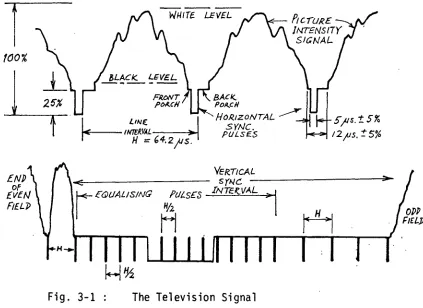
Chapter 3: Digitisation of Static Television Images.

The standard television monochrome signal in Australia is composed of 625 scanned lines of image, presented at a rate of 25 frames per second.

Each of the 25 frames is presented in two interlaced fields of 312 lines, 1

each field-sequence of sb th second duration. Each line is of 64 micro-seconds duration and is partly composed of a line-synchronising pulse of approximately 5 micro-seconds duration. (3.1). Vertical synchronising pulses occur at 50 Hz and are of approximately 500 ps duration. The start of an

interlaced field occurs at a half-line interval after the end of the preceding vertical synchronising pulse. During high-frequency transmission of television signals a train of line-synchronising pulses and equalising pulses (at twice line frequency) are inserted in the period of each vertical synchronising pulse. The presence of picture-intensity information gives the television signal

significant spectral components over the range zero to several MHz.

WHITE LEVEL

PICTURE INTENSITY

SIGNAL.

[image:15.555.66.489.459.767.2]

10 %

Typically the amplitude of the video signal is 1 Volt peak-to-peak, with the top three quarters of the wave-form reserved for the

picture-intensity signal, and the bottom quarter reserved for synchronising pulses. Thus a signal of - 0.3 Volts would represent zero picture-intensity (black) and a signal of- !Volts would represent the maximum picture-intensity (white). Clearly there should be a precise control of these maximum and minimum levels if the television camera is desired to be used as a measuring (photometric) camera.

The process of digitising a standard television signal so that it can then be stored in the memory of a computer can be shown to impose rather daunting requirements upon the designer of the electronic hardware. If the image of one monochrome frame of television is assumed to represent 256,000 (512 x 512) bytes of information, then the digitising hardware must transfer this data to a computer memory at an average rate of (256,000 x 25) nearly

8 Megabytes per second to maintain a complete record of a dynamic televised scene. For the purposes of obtaining repeatable digital images of microscope tissue-sections, there are fortunately several simplifying factors.

For tissue sections the televised field of view is generally a static image; thus the signal digitisation can be performed over an interval of many

successive frames, at a speed more appropriate to the cycle-time of common microcomputers (- lps). The diagram below, Fig. 3-2, shows three timing options that could be chosen if interlacing is ignored: Sampling time-Sequence =

1,2,3 n2-1, n?' The two important timing parameters to consider in these schemes are the total digitisation-time, T d , and the minimum time between sampling instants, t s . For a (128 x 128)-sample digitisation, T d and t s would have

- 13 - 1

69)

1

_

20 31 40 60 2"i-I

_

_ 3n4-/ , e .

CT

,---

411-10

?n+1 t2n4-1

etc.

r

nCtito

,)

o _n+I ---rt o

-2110

3,41 3ft 0

44 c)

1 sanynle/F_ramie

h(n-0+1 , etc .

G 0

-

-

n

samplesicrame

h24

o o

--

ED

----0

5 CO _{70 - 80} ' loC) ii

co

47

-

1.

sampiesjframe

471-3 4.772.

471

-

1

0 0 0 471

time/sample

2 -2,

.1 ...

T

d =4,n.lusecs.

=20

rilsec.

4

t s(min) = 2 X10 ps .

T

d(min) 142 33 C) secs.

2. t)

(b)

-2 T

d =2n.10secs.

time/sample =■120\-ernsec.

t

s(min)=-4ap s. T

d(min) z2.8 secs.

(c)

Td 2 eiecs.

20

time/sample = (4--n-)MSe.C.

t

_s(min

):=.'

10 S.

T

[image:17.556.46.514.44.398.2]

d(min) 'II 0:7 secs.

Fig. 3-2: Three (n x n) pixel digitisation sequence options for a static television image.

In keeping with international image-processing standards which favour pixellation at integral exponents of two (3.2), the pixel-value n shown in Fig. 3-2 above could be chosen as 2, 2' or 2 for a standard 625-line image. The sequence option chosen in this study is 3-26, with pixel-values of 128 and 256, a choice dictated by the existing instrument computer, an Acorn Model BBC-B fitted with 20K bytes of additional RAM.

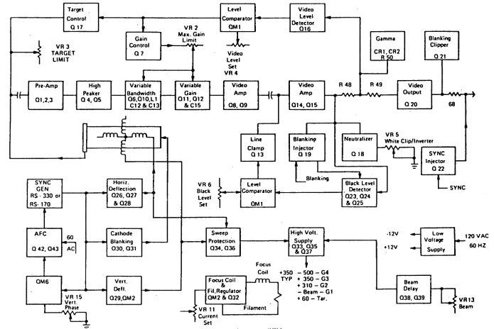
As mentioned above, there is a need for precise control of the gain and thresholds of the television camera if it is to be used as a measuring camera. The following feedback systems in the camera circuit are thus modified: (refer to the camera block diagram, Fig. 3-3).

(a) Automatic target-voltage system: this is disabled by clamping the feedback transistor Q17 in a cut-off condition, allowing manual control of the target-voltage by VR3. The target voltage is fixed at +30 Volts.

(b) Automatic gain-control system: this is disabled by clamping the feedback transistor Q7 in a cut-off condition, thus making gain manually controllable by the setting of VR2. The negative feedback applied to Q12

is reduced by bypassing its emitter series-resistor with a capacitor, thus maximising the gain in the variable-gain stage represented by Q11, Q12 and

C15. The automatic bandwidth control is left unaltered.

(c) Automatic black-level system: This system compensates for signal-level drift and dark-current drift due to temperature, tube age and target-voltage changes that occur when the auto-target voltage system is in operation. Since the target voltage is fixed and since the camera could be kept at a constant temperature (in its laboratory environment), it is decided to set the black-level manually and to monitor any variations due to tube age at intervals of no longer than one month. Accordingly the wiper of VR6 is disconnected from the output of QM1 and jumpered to the line-clamp FET, Q13.

As well as ensuring that the image-sensing device has well-controlled and stable operating parameters, it is essential to provide an accurately

[image:19.834.88.783.50.514.2]

FIG. 3-3 MTI-65 CAMERA Block Diagram

Blanking Clipper 021 Gamma CR1.CR2

R r

R 49 R 48

—e—Wo—•—+ •

68 • Video Output 020 Beam Delay

038,039 _{VR 13}

Beam -12V +12V Neutralizer 018 Black Level Detector 023. 024 & 025 VA 5 White Clip/Inverter SYNC Injector 022 Low Voltage Supply SYNC

... 120 VAC

IT 60 HZ Video Amp Video Amp Q8.09 High Peaker 0 4, 05 Pre-Amp

01,2,3

Variable Gain 011.012

& C15 014.015

Variable Bandwidth 06,010.1.1 C12 & C13

Line Clamp 013 VA 6 Black Level

Set OM I

Honor. Deflection 026. 027 & 028 Level Comparator SYNC GEN AS- 330 or

RS- 170

Blanking Injector

019

L

Blanking

Target Level

Control Comparator

017 • VR 2 GM I

Max. Gain

VR 3

Gain

Control Limit

_AL

TARGET 07 Video

LIMIT Level

Set VR 4

4

Video Level Detector 016 AFC 60 Vert. Dell. 029,0M2 0M6 VR 11 Current Set Filament Sweep Protection 034.036 VA 15 Vert. Phase High Volt. Supply 033 035

Ss 637

+350 —500-04

TYP +350-03 + 310— G2 — Beam — GI + 60 — Tar.

042.Q431 AC

•____ Cathode 01

Video

0-4 input

Sample

Fp

Hold

--PP-

SOC Analos

ADC

CLCK ' USER..

POkTi

4.6 MHz. Clock

6 bit

data

SYNC

SYNC Cla •

■-11. _{g bit}

cohtrol

bi te

PRINTER POkT

EOC

Level

Cc:int-n.)1

Losic

when the illumination filament-current is changed (normally after changing the objective lens power), provided best contrast for the most commonly-used tissue stain (Haematoxylin & Eosin) and provided illumination at a wavelength which is close to the points of maximum sensitivity of both the human eye and the vidicon.

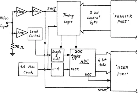
[image:20.555.67.506.440.740.2]

The instrument computer available for the task of signal digitisation and storage, an ACORN BBC-B, possesses a 10-bit ADC with an 8-bit conversion time of 4 milliseconds. Thus an interface is constructed with a much faster ADC (8 is. conversion) and parallel data-transfer to the computer; its block diagram is shown in Fig. 3-4. A clamp is used to present synchronizing pulses to the comparator at a predictable level and an I.C. video amplifier (National Semiconductors type LM733) is used to provide a signal gain of 2.0 to 5.0, to match the input signal to the input range of the ADC. The ADC chosen is a Ferranti type ZN448 with an on-chip 2.5 Volt bandgap reference.

Two computer programs have been written in 6502 machine code to breathe life into the hardware described above. They are:

(a) program 'FRAG', to control interface timing while monitoring the TV signal samples. This program operates with all computer interrupts disabled, since it is a time-critical task, and transfers signal samples to magnetic disk in four 16K-byte blocks in the case of 64K-pixel images to circumvent the problem posed by the computer's data-storage RAM which is limited to 16K bytes.

(b) program 'U' to display the image data rapidly (- 1 sec.) as an eight-colour digital image. An alternative data-display program, written in BASIC, has shown itself to be unconscionably slow (- 45 seconds), since such a display is usually required only as a quick visual check on system integrity.

Chapter 4 : Quantitation Using the Laplacian Operator

Two of the most frequently encountered problems in the analysis of microphotometric scans are those of simple counting and segmentation. Due to the loss of information inherent in the sampling and reconstruction processes (because of aliasing and the loss of higher spatial-frequency components), the need exists for a quantitative guide to thresholding: it is only when

statistically 'good' thresholds have been chosen that accurate segmentation and counting can be done.

The most simple and direct approach to threshold selection is based upon locating minima in the histogram of the scan data. If a substantial amount of

sampling-caused blurring of the scan data is present, this approach is inapplicable; a sharpening of the scan histogram can be carried out however using properties of small regions of the scan data based upon mathematical operators such as the

Laplacian, particularly if attention is restricted to a particular class of images, such as microphotometric scans.

The Laplacian operator in its original expression is derived from the vector differential operator V (del), by forming its scalar product with itself, V.V.

Since Vf(x,y,z) is the vector gradient of a function f (x,y,z),

= -Fiaf+k af

Dx Dy -.z, and V.Vf(x,y,z) is

the divergence of the gradient, the Laplacian:

3

2f a2f a2f V.V f(x,y,z) = V f(x,y,z) = —2- + —2- +

Dx Dy 3z

The equation V2f + k2f = 0 has several well-known forms that are invaluable in field theory (4.1), viz. for

- 19 -

k2 = 0 - Laplace's equation, k2 = +ve constant - Helmholtz' equation, k2 = -ve constant - Diffusion equation, and

k2 = constant x kinetic energy - Schradinger wave equation.

The function f in the case of microphotometric scan data is a scalar function of two discrete variables, the points at which the photometric data is sampled; it is useful to consider the physical meaning that VI assumes in such a case. The second partial derivative of a function of a continuous variable is often referred to as its curvature in that particular variable or dimension. For data sampled in two dimensions the Laplacian value at a point (i,j) is expressed in current literature as the absolute value of the difference between the value at that point, p(i,j), and the average of the adjacent eight neighbouring points, n 8 ,

where

1

j+1

ne =

272

Pi;) — Pij,) , (4,2). Such an expression

i-1 j-1

will give large values in highly discontinuous regions, where edges, holes and other dislocations exist in tissue sections for example, unless the central point

is within discontinuous regions that may be best likened to 'saddle' surfaces (of opposite curvature in two orthogonal directions) and regions of very high, uniform slope. To determine the frequency of occurrence of such central points a survey was made of twenty microphotometric scans of several types of natural tissue sections; the results are shown here in Table 4.1. The analysis program is attached in Appendix 2.

The program, 'LAP', calculates the number of anomalous 'saddle'-points by testing the products of pairs of differences between opposing neighbourhood edge-points, and the central value of that (3X3) neighbourhood. If either of the products is less than -99 then it is classified as anomalous. All scan values dealt with are integers in the range zero to one-hundred.

[image:24.545.99.506.151.722.2]

Table 4.1 : Statistics of Anomalous Laplacian Points in

Twenty Microphotometric Scans.

POINTS WITH

TISSUE TYPE

STAIN

LAPLACIAN,10

(% of total)

Human Prostate

H & E *

#1

4.44

112

2.46

113

2.76

114

20.1

115

0.59

SADDLE POINTS

(% of total)

3.22

2.32

1.85

11.3

0.49

POINTS OF

HIGH SLOPE

(% of total)

3.76

1.88

1.56

10.5

0.098

Human Skin Warthin-Starry

111

10.7

8.20

2.80

112

1.66

0.80

0.27

11

3

19.6

16.2

13.0

114

1.85

1.78

0.85

115

19.5

11.4

5.78

Human Breast

H & E *

# 1

1.98

0.83

0.73

# 2

1.54

1.12

0.12

# 3

0.37

0.22

0.024

# 4

0.39

0.20

0.049

#5

0.61

0.54

0

Pacific Oyster,

Timms

C.Gigas

#1

12.5

11.3

9.68

#2

12.8

8.95

5.63

113

13.4

10.1

8.10

#4

5.27

4.34

2.56

it 5

8.63

7.39

2.95

- 20 -

they have been first rejected as Laplacian or saddle-points, and if one-eighth of the sum of the absolute values of all differences (between the central point and its eight neighbours) exceeds the Laplacian difference-threshold, the 'similarity-parameter', S% in the program. This classification would typically be given to points possessing two groups of four neighbours

that are relatively very high and very low by roughly equal amounts.

Table 4.1 shows that the discrete form of the Laplacian operator is generally valid as a means of locating discontinuities in microphotometric scans; indeed the use of this operator to sharpen histograms of such scans and to locate thresholds for the counting of small, dark points in oyster tissue sections (representing metal-bearing granulocytes) is the subject of a recent publication by the author and colleagues (4.3). Nevertheless there is a disturbing trend in Table 4.1 for anomalous points to be present in numbers similar to the total of Laplacian points, prompting one to look for an operator yielding greater accuracy. Another feature of this table is that there is potentially useful information in the relative numbers of anomalous points, with regard to texture. In the scans of prostate tissue, for example, there is a consistently lower number of discontinuity-points in areas that are free of cancer; scan #5 is an instance of this. Scans #3 and #4 differed only in the depth of staining, so this is another factor that affects the results of counting with program 'LAP'.

An alternative edge-detection operator is the isotopic derivative form known as the gradient. For the continuous function f(x,y) it has a magnitude and direction given by {(%)+ 06.40and arta+ e9x1(

ai 7

(4.7).

[image:26.556.63.527.250.505.2]

All twelve scans are over prostate tissue sections and the table shows that points with a high gradient magnitude are far more common than points with a high Laplacian value. In contrast to the Laplacian operator the gradient operator is not strongly affected by tissue-staining, and there is no overlap between the counts for the two sets of four scans taken over the same slide, comparing two areas judged to be different from the clinical pathologist's viewpoint.

Table 4.2: Comparison of Laplacian and Gradient Point Numbers.

Scan title

Pathology (all Prostate)

Laplacian Gradient

(threshold =10, both as % of total) D. 81

D.B2 D. B3 D. B4

Cancer, light staining. 4.44 2.46 2.76 2.02 23.6 16.9 14.2 12.6 D.B11 D.B12 D.B13 D.B14 Cancer, heavy staining. 21.9 22.8 20.1 16.4 46.1 44.2 42.7 33.2 D.Y1 D.Y2 D.Y3 D. Y4 Benign, medium staining. 2.15 1.15 0.59 1.49 9.29 5.29 2.85 7.95

Other neighbourhood-operators that can be used in histogram-enhancement are the Roberts-Cross (4.2), various forms of the Laplacian taken over wider areas (4.4), and operators that select the maximum of differences of average values in pairs of horizontally and vertically adjacent 2x2 neighbourhoods. Alternative approaches to segmentation employ iterative methods to modify the histogram (4.5) and probabilistic relaxation of individual point values (4.6).

An operator that shows more promise as a means of enhancing textural detail is the Sobel operator (4.8), which will be considered at length in the next

- 22 -

CHAPTER 5: Texture Analysis of Tissue sections

Several definitions of image texture have been proposed, but as yet •

there is none that has been accepted universally. There have been several good reviews of texture (5.1, 5.2, 5.3); all of them agree that 'natural' texture is a stochastic or deterministic surface-property repeated over locales and that local properties can best be assessed by reference to the concept of a textural primitive. There is good evidence to show that image statistics beyond the second-order level are relatively indistinguishable by the human visual system (5.4), thus raising the hope that visual automata can achieve a level of

performance quite beyond the ability of human observers in the assessment of natural textures.

In the absence of well-defined shape or structural primitives a statis-tical approach to texture analysis is likely to be more effective; this is the case with the great majority of the biological tissue sections that the author has encountered. Biological organisms evidently have ordered structures, but such is their variability at all levels of size that a structural approach to their textural properties was judged to be unlikely to meet with success. Thus the problem becomes one of deciding which set of statistical features is likely to be most effective in providing a satisfactory analysis of the natural textures in tissue sections. Fortunately there is a good guide in the results of tests by Pratt, Faugeras and Gagalowicz (5.7) and by Faugeras and Pratt (5.8),

process. Classification of: four natural textures ( sand, grass, wool and raffia ) by this method was shown to be quite good (5.8); a simplification of the method arises from noting that the histogram moments of decorrelated fields are good discriminant features by themselves.

The operator chosen for decorrelation of the tissue-section scans in this study is the Sobel operator, which can be understood by reference to Figure 5-1 below : The Sobel value at each point 't' is given by

[image:28.556.64.485.183.422.2]

2 I

/2

St = [(p+2q+r-v-2w-x) 2 + (r+2u+x-p-2s-v) -]

Figure 5-1 : The (3X3) mask-size Sobel Operator

A program, 'SOBEL', was written to perform this decorrelation of the microphotometer scans; see Appendix 2.. The Sobel operator was chosen because it performs well in comparison with other edge-detection and thresholding operators such as the Kirsch, Roberts, Laplace and Prewitt operators (5.11). An extension of the mask-size (beyond the 3X3 level) was thought unnecessary in view of the relatively high signal-to-noise ratio (>100:1 ) of the microphotometric scans; this also confers greater computational simplicity and speed.

[image:29.556.55.517.39.801.2]

- 24-

Figure 5-2 : Photograph of the Prostate Tissue Section, Slide Si, that was scanned microphotometrically. Several areas of the tissue ( shaded ) are carcinomatous.

The test objects for texture analysis were two Haematoxylin/Eosin-stained, 5 pm.-thick, stepped sections of human prostate tissue, slides

Si

and S2. Twenty-eight areas of 1.6me were scanned microphotometrically in 10

pm.

steps over square grids of 16,384 points each. Eight scans were carried out initially on Si over areas judged to be texturally different by a non-specialist. This naive selection of areas was then re-scanned after the tissue section had been re-stained to test for variation of the texture indicators. Slide S2 was

prepared six months after Si, during which time the tissue block was subject to the minor effects of storage in paraffin at room temperature. Approximately 30 pm. of the block was removed in cleaning the face to be sectioned for the preparation of S2; the appearance of S2 after Haematoxylin/ Eosin staining

was very similar to, but not identical with, Slide Si. Twelve 1.6mm2 areas were scanned microphotometrically on S2, following a dispersed selection similar

to that on Si. As is the usual practice with (H & E) stained tissue, green light (KODAK Wratten Filter No. 58) is used to illuminate the tissue for maximum contrast.

At the start of each series of scans the instrument is allowed a half-hour to stabilise thermally and the photometer ADC is calibrated. The measuring stop was adjusted to a width of 12 pm., referred to the image (tissue-section) plane, and the luminous-field stop was adjusted to a width of 30 pm. in the same plane to minimise diffraction disturbances from its edge. A 100% transmission reading was obtained close to each scan area, through an area of slide clear of tissue within a 60 pm. radius. At the end of each scan the data was rejected if more than 1% of the 16,384 transmission readings were in excess of 100%. In this way a reasonable degree of standardisation was achieved.

(a)

Scan LoF- (Bert;jn)

(10

Sca n

LOF--63 (Cancer)

- 26 -

[image:31.554.35.515.67.799.2]

Each scan was processed with the Sobel operator, as outlined above, and the same statistics were obtained from the processed scans. The Sobel-processed scans showed enhancement of discontinuities in the original scans, as can be seen by the digital image pairs of Figure 5-3.

Figure 5-3 : Two digital-image pairs at the same thresholds, ! showing the edge-enhancement due to processing with a Sobel operator. Unprocessed scans are at left, processed at right.

Tables 5.1 and 5.2 show the statistics for the unprocessed and

processed scan data, respectively. All of these scan areas were examined by medical specialists so that a 'cancer' or 'benign' classification could be given. The letter C or B indicates this expert opinion; a small 'm' subscript indicates a majority opinion.

[image:32.555.57.534.146.780.2]

Table 5.1 :

SCAN Area Pathology

Statistics of Twenty-Eight Microphotometric Scans of Prostate Tissue

Mean Variance Skewness Kurtosis Span

LOF-81 * 1. C 81 61 0.93 3.22 26

LOF-B2 * 2. C 83 54 0.73 3.18 26

LOF-G1 * 3. C 78 70 0.88 2.90 27

LOF-G2 * 4. C 75 53 1.27 4.20 24

LOF-R1 *11. B 76 80 1.34 4.08 32

LOF-R2 Cm 80 115 0.64 2.29 31

LOF-Y1 *12. B 84 39 0.13 3.98 21

LOF-Y2 *13. B 81 45 0.85 4.43 26

LO-81 * 5. C 65 240 1.11 2.91 49

L0-B2 * 6. C 64 207 1.12 3.08 46

LO-Gl * 7. C 62 259 0.96 2.80 52

L0-G2 * 8. C 58 181 1.71 4.98 46

LO-Rl *14. B 61 189 1.72 4.89 49

L0-R2 Cm 67 312 0.80 2.05 49

LO-Yl *15. B 69 87 1.01 4.40 32

L0-Y2 *16. B 67 96 1.48 5.23 39

LOF-B3 * 9. C 78 72 0.65 3.20 30

LOF-B4 *10. C 73 72 1.05 3.72 28

LOF-B5 *17. B 83 27 0.46 5.36 17

LOF-B6 *18. B 83 21 0.42 5.56 15

LOF-G3 Bm 80 55 0.69 3.73 26

LOF-G4 Bm 76 47 0.93 4.64 24

LOF-V1 Cm 78 77 0.65 2.74 30

LOF-V2 Cm 80 102 0.50 2.13 30

LOF-W1 Bm 75 67 1.40 4.73 30

LOF-W2 Bm 76 44 1.30 5.55 21

LOF-Y3 *19. B 75 52 0.83 4.67 24

LOF-Y4 *20. B 74 66 0.85 4.04 29

C = Cancer B = Benign

Cm = Cancer, admixed with other pathological classes

[image:33.557.55.520.174.758.2]

- 28 -

Table 5.2:

SCAN Area

Statistics of Twenty-Eight Sobel-processed Scans

Pathology Mean Variance Skewness Kurtosis Span

S.LB1 *•1. C 34 598 0.93 3.17 78

S.LB2 * 2. C 31 473 0.95 3.47 69

S.LG1 * 3. C 35 733 0.87 2.81 85

S.LG2 * 4. C 30 566 1.03 3.35 75

S.LR1 *11. B 27 810 1.57 4.74 92

S.LR2 Cm 38 1000 0.91 2.80 100

S.LY1 *12. B 24 358 2.03 8.56 57

S.LY2 *13. B 25 449 1.99 7.44 70

S.B1 * 5. C 44 1145 0.78 2.54 109

S.B2 * 6. C 52 1087 0.87 2.75 107

S.G1 * 7. C 48 1077 0.60 2.38 106

S.G2 * 8. C 38 1029 1.05 3.14 103

S.R1 *14. B 28 831 1.60 4.92 93

S.R2 Cm 39 1139 0.94 2.86 108

S.Y1 *15. B 30 508 1.63 6.13 72

S.Y2 *16. B 28 628 1.93 6.61 85

S.LB3 * 9. C 36 518 0.88 3.44 74

S.LB4 *10. C 30 531 1.04 3.71 72

S.LB5 *17. B 19 205 1.81 8.21 '43

S.LB6 *18. B 19 164 1.32 5.21 40

S.LG3 Bm 30 479 1.31 4.57 69

S.LG4

B.

27 416 1.50 5.29 66

S.LV1 Cm 34 613 1.00 3.53 79

S.LV2 Cm 32 774 1.18 3.78 90

S.LW1 Bm 27 509 1.53 5.30 72

S.LW2 Bm 25 386 1.65 6.10 62

S.LY3 *19. B 22 346 2.34 10.11 55

S.LY4 *20. B 28 490 1.80 6.72 72

C = Cancer B = Benign

Cm = Cancer, admixed with other pathological classes

marked in tables 5.1 and 5.2 with an asterisk and a numbered sequence. The

complete results of the above tables were used to prepare several

feature-space diagrams, Figs 5-4 to 5-7, which show four scatter-plots by which the

statistics were examined to proved a basis for classification. A two-fold

partition of these scatter-plots can be made into the classifications 'Cancer'

and 'Benign' with varying degrees of success. A program, 'BAT', was written

to provide a quantitative guide to the separation of these two classes (see

Appendix 2); table 5.3 shows these separation statistics, known variously as

Bhattacharyya or

Mahalanobis

distances in the literature (5.8, 5.9, 5.10), for

all possible dissimilar pairs of statistics that are listed below:

UNPROCESSED DATA SOBEL-PROCESSED DATA

. 1. Mean transmission 6. Mean

2. Transmission Variance 7. Variance

3. Skewness 8. Skewness

4. Kurtosis 9. Kurtosis

[image:34.556.55.538.327.755.2]

5. Span 10. Span

Table 5.3: Mahalanobis Distances for Pairs of Scan Statistics, Drs

STATISTIC (s)

STATISTIC (0 2 3 4 5 6 7 8 9 10

1 10.3 1.90 44.5 5.85 82.2 23.1 160 93.9 19.2

2 6.97 41.7 9.15 107 17.0 162 91.2 13.1

3 48.6 4.49 55.0 18.0 160 103 18.0

4 40.3 63.6 44.8 186 125 43.0

5 122 27.7 160 94.8 22.4

6 73 170 104 74.7

7 160 90.6 14.0

8 168 160

9 91.8

SEQUENCEII—S STRT. N08.TS.9

SCALE NOS.T4.1 + = Cancer o _{= Benign}

•

+

4+

0

... V)

Sobel Skewness

Illillill

Im•••

- 30 -

SEQUENCEs1-211 • STAT. NOS.T8.9 SCALE NOS.T4,1 +

•

e

•

9 8 7 6 5 4 3 2 1

•

•

'CU

-0

+ = Cancel = Benign

Sobel Skewness

I1 Milli

•

0

• •

•

₄

11108.?4.11 _{SEQUENCEs1-29} SCALE NOS.T1.5.1

Kurtosis

111111111

•

+ = Cancer * = Benign

• 4 +0 •+ 41. 9 8 7 6 5 4 3 2 1

0 1.0 2.0 Fig.5-4: Feature-space diagram, Sobel Skewness vs. Sobel Kurtosis. Mahalanobis Distance= 168

0 2.0 4.0 6.0

Fig.5-5: Feature-space diagram, (Unprocessed) Kurt. vs. Sobel Kurt. Mahalanobis Distance= 186

1.0 2.0 Fig.5-7: Feature-space diagram, Sobel Skewness vs. Sobel Kurtosis. Lightly-stained series, 8 scans. 4

3 2 1

0 STAT. MO8.T8.9 _{SEQUENCEI9-16}

SCALE NO8.T4.1

+ = Cancer • = Benign

•

•

•

JD 0 Cl) •+ Sobel Skewness

1 Ililli) 0 1.0 .0

Fig.5-6: Feature-space diagram, Sobel Skewness vs. Sobel Kurtosis. Heavily-stained series, 8 scans.

analysis of covariance and can be understood by reference to Appendix 4 and standard texts on statistics and clustering analysis (5.5, 5.12). The Drs value for the case (r = 4, s = 8) provides support for the inclusion of the histogram moments of unprocessed data in the feature vector; the reason for statistic no. 4, the kurtosis of the unprocessed scan histogram, being such an effective texture-feature is not understood by the author and could well serve as an interesting topic for further research. Another interesting separation value is

D8,10, whose relatively high level was quite unexpected.

Many other natural textures could possibly be classified rapidly by

the above method; future work will broaden the field of application and hopefully shed light on the unanswered questions above. A considerable increase in speed will result from the use of digitised television scans and the conversion of

the decorrelation program to machine code. Program SOBEL is currently in BASIC and takes 15 minutes to decorrelate a 16,384 - point scan. For the small

number of areas scanned in this study it has been shown that the higher

- 32 -

Chapter 6 : Microspectrophotometry

The properties of a specimen that can be measured with a micro-photometer are wavelength-dependent. The useful range of wavelengths of microscope optics is from about 300 to 1100 nm., spanning three regions: the ultra-violet (300 to 400), the visible (400 to 700) and the near infra-red (700 to 1100 nm.). Thus it was decided to couple the MPV2 microphotometer to a monochromator, when an Optica type CF4 was made available in 1982, to make possible the analysis of microscope specimens by microspectrophotometry.

A typical spectrometer consists of an entrance aperture, a collim-ating element, a dispersing element, a focussing element and an exit aperture. All of these components were available in the Optica CF4, as well as sample compartments placed just after the exit aperture and an obsolete type of photo-detector. The collimating element serves to make all the rays passing through the entrance slit parallel and the dispersing element acts as a filter to separate light rays according to their wavelength.

The expression relating an observed spectral power distribution 1(X) to the instrumental profile F(X) and the spectral power distribution of the source of radiation S(x) is one of convolution:

u = co

1(A) = 2.

f

S(u) F (A- u u = o

Two spectral lines may be regarded as resolved if they can be

detected as two lines without the aid of a deconvolution (working backwards to S(A) in the above equation) or knowledge of the instrument profile. The Rayleigh criterion is that two diffraction-limited profiles, with zeros on either side of their principal maxima, are resolved if the zero of one is superimposed on on the principal maximum of the other. Thus the resolution of a spectrometer which can just resolve two maxima at A l and A2 is defined as

Michelson Fourier spectrometers Field- compensated

multiplex spectrometers

Fab,ry- Perot Etalons

Plane diffraction

Gratings 10

Eten

du

e

(cm

2

s

te

ro

d

ia

ns

)

10-1

and the resolving power as

R

=

Apart from resolving power, the other basic instrumental factor of a spectrometer to be considered is its flux-gathering power, or etendue. Etendue is conserved in an ideal spectrometer; there will always be one limiting aperture in the instrument which defines one angle explicitly and all the others implicitly. A diagram showing the limits of etendue and resolving power of several common types of spectrometer is shown below by Fig. 6.-1, taken from a text by James and Sternberg (6.1).

Several methods of expressing optical absorption are in current use, but all of them are based on the equation a = k logio Io , where

100.— Upper limit set by area of available detectors

Prisms

I I I I I I t iJ

[image:38.554.90.496.319.672.2]

103 104 10 5 10 6 10 7 109 Resolving power

Figure 6-1 : The Performance Limits of Several Types of Optical Spectrometer in Common Use.

HYDROGEN LAMP TUNGSTEN LAMP

YELLOW FILTER

PHOTO - DET E CIO; - 34 -

't' is the optical path-length in the medium and C is the concentration of the absorbing species in moles/litre.

Term Symbol Equation

I

Transmission T T = To

Absorption A A = I - T

Optical Density O.D. 0.D.= logio (TR)

Extinction Co-efficient a a = [logio

(NA

Molar Extinction Co-eff. E

e =

[logio

The OPTICA CF4 is a single-beam, manually-operated spectrophotometer

GRATING SLIT I ft SPEC I MEN-CHANGE CONTROL SPECIMEN V ROD

[image:39.556.41.536.146.626.2]

COMPARTMENTS

Figure 6-2: The Optica CF4 Spectrophotometer, before the removal of the sample/measurement section.

A bench with a sliding table was made to support the monochromator so that it could be quickly changed with the usual light-source of the microphotometer, a 100-Watt tungsten lamp. The alignment of the monochromator output to the microscope so that it could form a stationary illuminated field as the wavelength was changed at the specimen stage was difficult, mainly due to

the monochromator's mass, - 100 kg. Once this was done any further movement was restricted to translation, directly in or out. By using the CF4

monochromator as an alternative illuminator for the MPV2 microphotometer in this way the possibility of stray light entering the system was much reduced.

A plane diffraction grating with 600 lines/mm (15,000 lines/inch) is used in the Optica CF4 and covers the spectral range 185 to 1000 nm. The resolving power of a grating, where N is the number of lines in the grating and m is the order of diffraction, is given by (6.3):

R = Nm

The plane grating can be regarded as a row of equidistant slits transmitting a plane wave of light parallel to the plane containing the slits. Each slit emits a series of Huygenian wavelets which expand in all directions; the wave-fronts are envelopes of these wavelets and will have angles to the plane of the grating in some way proportional to m and to the inverse of the slit separation, S.

The exact relation is given by:

mA = sin() + sine

[image:41.555.69.460.93.274.2]

- 36 -

Table 6.2: Calculated Angular Spread of Several Successive Orders

A (nm.)

0 (deg.)

m = 1 m = 2 m = 3

400 13.9 28.7 46.1

500 17.5 36.9 64.2

600 21.1 46.1 > 90

700 24.8 57.1 > 90

800 28.7 73.7 > 90

The considerable degree of overlap here indicates why only the first order of diffraction is used in the CF4, as in many spectrometers. An 0R2 glass filter

is supplied with the CF4 to remove the second spectral order when measurements are being taken at wavelengths greater than 620 nm. Thus the attainable resolving power of the CF4 can now be calculated; the number of lines in the grating is

(length, 4 cm; x N) 2.4 x 10", so

Resolving Power = 24,000

Thus it should be possible to resolve details of - 0.02 nm. at a wavelength of 400 nm. (extreme blue). The figure given by the manufacturer is in fact

0.05 nm. In view of the age of the monochromator and the maximum resolution likely to be required in usual applications (-1 nm.), these figures for the attainable resolving power were regarded as more than satisfactory. Experience has since shown that it is the total light available from the monochromator's 50 Watt Tungsten lamp that constitutes the limiting factor in most applications: resolving power is often sacrificed for illumination by opening the slits.

means of a geared stepping motor attachment to the original manual control The instrument computer monitors the wavelength, to a resolution better than 1 nm., by means of the third channel of its four-channel, 10-bit ADC. This ADC reads the output of a 10-turn, 10K0 potentiometer whose shaft is geared to the main gear-wheel of the wavelength-control shaft, and to which a highly-regulated reference voltage is applied. The equation relating the monochromator wavelength to the value read by the ADC, A3, has been found by measurement

to be:

A

= { . 7 4) +

15

This relationship is an integral part of a series of programs that have been written to perform the collection of spectra from areas of specimens down to the level of a micron square. Program 'SPAA' is attached, in

Appendix 3 . The light-intensity signal detected by the MPV2 photometer tube is digitised by channel 1 of the instrument computer's ADC, in the usual way; depending upon the particular measurement a degree of averaging is carried out to improve the signal to noise ratio.

Since the instrument is of the single-beam typelprogram SPAA collects a reference spectrum from a clear area of the microscope slide before the

specimen itself is examined. All light readings from the specimen are

expressed as a ratio to the readings obtained at the same wavelengths in the reference spectrum.

3 .000

Abs

.----

1 \II

1.00 1.00

400 0 .00

800

700

600

500

-38-

[image:43.554.69.542.126.784.2]

535 nm. The results of this work were presented at the 1984 Symposium of the Royal Australian College of Pathologists in Perth (6.4). An absorption spectrum of a sample of Neodymium-containing glass is shown below, Fig.6-3, illustrating the result obtained when an X-Y plotter was (Aed. Spectra are normally printed out via an ITT Model 43 Teletype.

Conclusion

Various methods by which microscopic observations can be made more quantitative, rather than qualitative, have been discussed in this study. It is to be expected that this trend, which has so far been most evident with X-ray microanalysers and electron microscopes, will be more apparent in future with light-optical and accoustic microscopes as their electronic component becomes a more integral part of their design. The instruments of this type will not make the operator redundant however; quite the opposite can be expected : the advent of "intelligent" micro-scopes will enhance the quality of microscopic observations.

Two methods of digitising microscope images have been demon-strated and their limitations have been discussed. Television scanning has an inherently low level of aliasing error, due largely to the near-Gaussian electron-density profile of its reading beam. It suffers from a low signal-to-noise ratio and poor linearity however, particularly if a Vidicon tube is used. Microphotometric scanning has neither of these disadvantages and has a very good geometrical accuracy as well, but it is much slower. Its aliasing error can potentially be reduced by the aperture-modification indicated and there is great scope for improvement to the scanning speed by changes to the stepping-stage hardware.

- 40 -

As has been shown in Chapter 5 there are good statistical features for texture analysis when structural features are either absent or so variable as to be quite unreliable indicators. It is often advant-ageous to filter out visual information initially, as was done with the prostate tissue colouring, to assist in information reduction. Optical enhancement is also possible with histochemical staining of the tissues, and many aspects of these techniques remain to be evaluated. Is there, for example, some degradation of the textural statistics listed in Chapter 5 that can be shown to be due to the use of a non-Gaussian scanning

aperture ? The role of colour-texture in portraying the pathological state of the tissue also remains to be studied; the tissue-stain used was a red/blue type while the illumination used was almost a spectral green.

There are thus limitations in image acquisition in image acquisition and optical analysis, which may be said to be problems of hardware, and there are many unexplored avenues of image analysis and data-reduction, which are essentially problems of the software. Of these two types of problems, it is the author's view that those relating to software are the furthest from adequate resolution. Advances in electro-optical imaging devices have made possible a very accurate recording of the light-microscope image; the subsequent treatment of this information in an attempt to mimic and surpass human comprehension with visual

APPENDIX 1 : Television Digitisation Programs

100 REM •** FRAME-GRABBER PROGRAM "FRAG" 110

120 REM .... INITIALISATION

130 REM .... USER VIA - Port A = Output, Port B = Input 140 REM .... PB6=Composite SYNC PB7=E0C from ADC _/= 150

155 *FX111,1

160 DX=178:?&79=DX:REM...No. of times each TV line is sampled 170 HX=4:?878=HX:REM...Vert. jmp between samples

180 MX=83000:?&7A=00:?&71(=&30:REM...Memory-base

190 NX=20:?87C=NX:REM...No. of lines initially ignored 200 SX=128:?&70=SX:REM...No. of TV lines sampled 205 IX=2:?87E=IX:REM...Set interlace counter 310

320 DDRA=8FE63:DDRB=8FE62 330 PRTA=8FE61:PRTB=8FE60 340

350 FOR PASS=0 TO 3 STEP3 360 PX=87200

370

380 OPT PASS 390 .GRAB 395 LDY NO 400 .INIT

410 LDA NUF:STA DDRA \ Set PRTA all outputs 420 LDA NUO:STA DDRB \ Set PRTB all inputs

430 LDA VD:STA 87F:LDA87C:STA877 \ temp-store for SX and MX 440 LDA N87F:STA &FE4E:STA 8FE6E \ Disable all VIA interrupts 460

480 .PLOOP:LDA PRTB \ Wait for VSYNC event 490 ASL A:ASL A \ c <-- PB6

500 BCS PLOOP

510 ASL 1FFFF \ 6 usec. delay

520 LDA PRTB \ look for SYNC again 530 ASL A:ASL A

540 BCS PLOOP -

542 DEC 87E:BNE PLOOP \ Eliminate interlace

550 LDA 877:STA 87C \ VSYNC found; set line-delay NX 555 LDA 87F:STA 871' \ Set no. of lines sampled too 560 .PLUP:LDA PRTB \ Wait for VSYNC to end

564 ASL A:ASL A:BCC PLUP 570

- 42 -

Program 'FRAG' ( cont'd )

600 .SETHOR \ Set up 74LS161's with current value of DX 610 LDA &79

620 STA PRTA 630

660 LDA #&40 \ Set bit6 of accum.

670 .DLOOP \ Wait NX lines before looking at ADC 680 BIT PRTB

690 BNE ['LOOP

700 DEC &7C \ Decrement line-counter,

NX

720 BNE DLOOP

730

780 .HLOOP \ Wait for EOC of ZN448 on PB7 784 LDX

788 .HL

790 LDA PRTB:ASL

A

800 BCC HL 802 DEX: BNE HL 810

820 .SNAP \ Collect result from ADC and eject P86 830 ASL A:LSR A:LSR A

840 STA (&7A),Y \ and save it in memory

850 INC PA:BNE FWRD \ Increment mem.-pointer 860 INC &7B

870 .FWRD

880 DEC &7D \ Decrement sample-counter SX 890 BNE HLOOP

900

910 LDA 11&02:STA &7E \ Reset interlace counter

915 .SSTEP:DEC &79 \ Decrement line-sample counter DX 917 LDA879:CMP#50

920 BNE PLOOP \ Do next frame 930

940 LDA ii&FF:STA &FE4E \ Re-enable all interrupts 950 RTS

960 970 ] 980 NEXT 990

1000 CALL GRAB

2050 SOUND 1,-15,77,11 2060 CHAIN "VU"

3000 END

•

PROGRAM ' U ' : Rapid Display of TV scans

40 q2C90=811011000 44 q2C94=815051404 46 MC98411011000 48 q2C9C=815051404 49 !A2CA0=810100000 50 MCA4411110101 51 MCA8=&14140404 52 q2CAC=115150505 54 FOR NX=0 TO 255

55 ?(g2B0O+NX)=?(82C90+NXDIV8) 60 NEXT NX

70 MC=0:REM...00LOUR OFFSET 100 MODEO

105 *FX111,0

110 REM...SCREEN / ARIES DISPLAY 120 OSBYTE=UFF4

140 FOR PASS=0 TO 2 STEP2

144 PX=SCOO 150 [ OPT PASS 200 .DIS

204 LOAN&40:STA&84:LOANA30:STA&85 \ Set top LHS of screen 208 LOA00:STASBA:LDA#830:STA8811 \ set data base pntr 212 LOAN&10:STAHD \ Set stripe cntr

214 .LLP

216 LOAttA6F:LBXN&81:JSR OSBYTE \ turn on ARIES ram 220 JSR BLOT

224 LDAMF:LDXNUO:JSR OSBYTE \ turn off ARIES ram 228 JSR GOB

232 DEMO \ see if all stripes done 236 BNE LLP

240 .FIN RTS 280 .GOB

400 .COL \ S-R to put 1 blocl, of bytes on to screen

404 LOA#0:STAA86:STA882:STAH7

- 44 -

Program ' U ' ( cont'd )

420 .SS

424 LDA#820:STAA8F \ Set cntr1=32 428 .RR

432 LDA#&04:STAHE \ Set cntr2=4 436 .00

440 L0Y886 \ collect data index

444 LDA(888),Y:ADCHC:TAX:LDA&2800,X:ASLA \ make LHS nibble 448 STA&87:STY&86 \ save data & data index

452 TYA:CLC:ADC#&80:TAY .\ add 128 to data index

456 LDA(&88),Y:ADCA8C:TAX:LDA&2800,X \ make RHS nibble 460 0RA887:INC886 \ form scrn-byte 8 incr. data index 464 LDYS82 \ collect screen index

468 STA(&80),Y:INY \ place byte on screen 472 STA(&80),Y:INY \ & update scrn index 476 STY882 \ save scrn index

480 DECHE \ decr. cntr2 (4 times) 484 BNE 00

488

492 LDY00:STY&82 \ reset scrn index & keep data index 496 LDA880:CLC:ADC#&80:STA&80 \ add 640 to scrn pntr 500 BCC BB:INC&81

504 .BB INC&81:INC&81

508 DECHF \ decr. cntrl (32 times) 512 BNE RR

516

520 INC&89 \ incr. data pntr by 256

524 LDA&84:CLC:ADC#&08:STA&84:STA&80 \ add 8 to top-scrn pntr 528 BCC DD:INC&85:LDA&85:STA&81 \ & reset (&80,&81)

532 .DD LDA&85:STA&81

536 LDA#0:STA&86 \ reset data index 540 DECA83 \ decr. cntr3

550 BNE SS 560 RIB 670

680 .BLOT \ Block-transfer S-R

684 LDA#0:STA&88:LDA#&2C:STA&89 \ set tar9et=&2C00 690 LDX#&04:LOYH0

700 .LPA

710 LDA (&8A),Y:STA (888),Y:INY 720 BNE LPA

730 INC &8B:INC 889:DEX 740 BNE LPA

750 RIB 760