City, University of London Institutional Repository
Citation
:
Zhu, H., Russell, R. A., Saunders, L. J., Ceccon, S., Garway-Heath, D. F. and
Crabb, D. P. (2014). Detecting Changes in Retinal Function: Analysis with Non-Stationary
Weibull Error Regression and Spatial Enhancement (ANSWERS). PLoS ONE, 9(1), doi:
10.1371/journal.pone.0085654
This is the published version of the paper.
This version of the publication may differ from the final published
version.
Permanent repository link:
http://openaccess.city.ac.uk/4994/
Link to published version
:
http://dx.doi.org/10.1371/journal.pone.0085654
Copyright and reuse:
City Research Online aims to make research
outputs of City, University of London available to a wider audience.
Copyright and Moral Rights remain with the author(s) and/or copyright
holders. URLs from City Research Online may be freely distributed and
linked to.
Non-Stationary
Weibull
Error Regression and Spatial
Enhancement (
ANSWERS
)
Haogang Zhu1,2*, Richard A. Russell1, Luke J. Saunders1, Stefano Ceccon1, David F. Garway-Heath2,3, David P. Crabb1
1School of Health Sciences, City University London, London, United Kingdom,2Institute of Ophthalmology, University College London, London, United Kingdom, 3National Institute for Health Research Biomedical Research Centre for Ophthalmology, Moorfields Eye Hospital NHS Foundation Trust and UCL Institute of Ophthalmology, London, United Kingdom
Abstract
Visual fields measured with standard automated perimetry are a benchmark test for determining retinal function in ocular pathologies such as glaucoma. Their monitoring over time is crucial in detecting change in disease course and, therefore, in prompting clinical intervention and defining endpoints in clinical trials of new therapies. However, conventional change detection methods do not take into account non-stationary measurement variability or spatial correlation present in these measures. An inferential statistical model, denoted ‘Analysis with Non-Stationary Weibull Error Regression and Spatial enhancement’ (ANSWERS), was proposed. In contrast to commonly used ordinary linear regression models, which assume normally distributed errors,ANSWERSincorporates non-stationary variability modelled as a mixture ofWeibulldistributions. Spatial correlation of measurements was also included into the model using a Bayesian framework. It was evaluated using a large dataset of visual field measurements acquired from electronic health records, and was compared with other widely used methods for detecting deterioration in retinal function.ANSWERSwas able to detect deterioration significantly earlier than conventional methods, at matched false positive rates. Statistical sensitivity in detecting deterioration was also significantly better, especially in short time series. Furthermore, the spatial correlation utilised inANSWERSwas shown to improve the ability to detect deterioration, compared to equivalent models without spatial correlation, especially in short follow-up series.ANSWERSis a new efficient method for detecting changes in retinal function. It allows for better detection of change, more efficient endpoints and can potentially shorten the time in clinical trials for new therapies.
Citation:Zhu H, Russell RA, Saunders LJ, Ceccon S, Garway-Heath DF, et al. (2014) Detecting Changes in Retinal Function: Analysis with Non-StationaryWeibull
Error Regression and Spatial Enhancement (ANSWERS). PLoS ONE 9(1): e85654. doi:10.1371/journal.pone.0085654 Editor:Steven Barnes, Dalhousie University, Canada
ReceivedOctober 10, 2013;AcceptedNovember 28, 2013;PublishedJanuary 17, 2014
Copyright:ß2014 Zhu et al. This is an open-access article distributed under the terms of the Creative Commons Attribution License, which permits unrestricted use, distribution, and reproduction in any medium, provided the original author and source are credited.
Funding:This report is independent research arising from a Research Fellow Award supported by the National Institute for Health Research, National Health Service, United Kingdom. The views expressed in this publication are those of the authors and not necessarily those of the National Health Service, the National Institute for Health Research or the Department of Health. The funders had no role in study design, data collection and analysis, decision to publish, or preparation of the manuscript.
Competing Interests:A provisional UK patent application (1311310.5, a retinal function analysis software) was filed and ANSWERS is part of analytical methods in the software package. The authors can confirm that this does not alter their adherence to all the PLOS ONE policies on sharing data and materials. * E-mail: [email protected]
Background and Significance
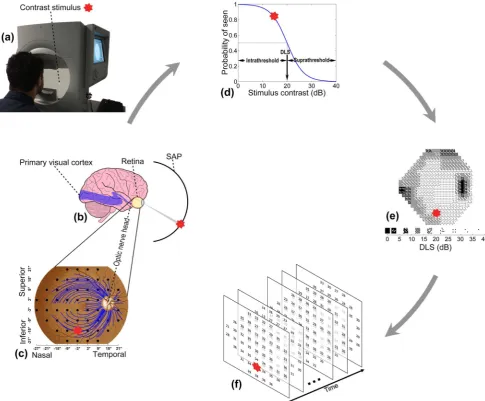
In recent years great strides have been made in understanding ocular diseases in the research laboratory andin vivo, leading to the elucidation of neuro-regenerative processes and even reversing blindness in some conditions.[1–4] The retina, uniquely, is an accessible and directly visible extension of the brain and, therefore, retinal research is becoming a focus for unravelling the complexity of other neurological changes such as those observed in Alzheimer’s disease,[5,6] multiple sclerosis [7,8] and Gaucher disease.[9] The primary goal in the management of most eye conditions is preservation or improvement in visual function. An established reference test for visual function, namely the visual field, is Standard Automated Perimetry (SAP; Figure 1a). SAP measures the differential light sensitivity (DLS), across a person’s retina and the corresponding visual pathway (Figure 1b,c). Unfortunately, development of computational and statistical methods for analysing data from SAP has not kept pace with the
Current methods for detecting change in series of DLS measurements are inadequate because they do not sufficiently address the complexity of the data,[19] notably non-stationary variability and spatial correlation. SAP measurements of retinal function are indirect because of the psychophysical processes involved – a person’s response depends on the probability of perceiving and responding to a light stimulus (Figure 1d). The consequence is considerable variability that increases as DLS deteriorates with the disease progresses, eventually becoming censored in blind regions.[20–22]. For instance, when DLS is healthy at 32 dB, the repeat measurement range (90% confidence interval) is 7 dB (26 dB to 33 dB), while this range increases to 18 dB (5 dB to 27 dB) when the DLS deteriorates to 20 dB. This
[image:3.612.63.549.61.462.2]changing variability over time is referred to as ‘non-stationary measurement variability’. Furthermore, SAP measurements are made in a regular grid across a patient’s field of view, but this grid does not respect the anatomical arrangement of the retinal nerve fibres that transmit signals from the retina to the brain (Figure 1c).[23] The division of the grid by retinal nerve fibres results in correlation between spatially-related locations. There are prescriptions for modelling this unique spatial process,[24] but they have yet to be incorporated into analysis of series of SAP measurements over time. Therefore, without taking into account these statistical properties, detection of change in retinal function with current methods is often delayed, or requires more clinic visits than should be necessary.[25]
Figure 1. Visual field measured by standard automated perimetry (SAP).(a) Contrast stimulus from SAP is projected on different locations of retina. The response from subject is captured when the stimulus is perceived. (b) SAP assesses differential light sensitivity (DLS) of the retina and corresponding visual pathway. (c) DLSs are measured at various locations (dots) on the retina. The point (0u,0u) indicates central vision that corresponds to the fovea on the retina. Optic nerve head is the anatomical blind spot. The test locations are not only correlated to their neighbours but also by the optic nerve fibres (some of which are shown as blue curves) passing through them. The whole visual field can be divided into superior and inferior hemifields on vertical and nasal and temporal regions on horizontal. (d) The DLS at a location on the retina is derived at the 50% probability of the visual system responding to a contrast stimulus and is related to the biological response to light of relay neurones in the visual pathway. (e) The DLS is measured in log scale, which in Humphrey Field Analyzer (Carl Zeiss Meditec Inc, Dublin, CA, USA) is calculated as dB =10 log10ð10000=ðA{31:6ÞÞwhereAis the luminance of the stimulus in apostilbs and 31.6 apostilbs is the background luminance. The DLS ranges between 0 dB (high contrast stimulus, blindness) and around 35 dB (low contrast stimulus, healthy) and is displayed as a conventional gray-scale plot. Darker shading represents lower DLS. (f) Measurements of DLS over time form a complex spatial-temporal time series.
To address these issues we propose an analytical approach to handle the variability structure in SAP data and also capture the information about the spatial process underpinning changes in the visual field. This new computational method, analysis with non-stationary Weibull error regression and spatial enhancement (ANSWERS), is designed to accurately identify changes in SAP measurements acquired over time (Figure 1f). Further, the method can be adapted to investigations of new therapies, so that changes before and after an intervention can be detected. In this study we applied the technique to large scale clinical data sampled from more than 75,000 patients in electronic health records. Specif-ically, we examine the hypothesis that ANSWERS can detect change in retinal function more rapidly than widely used methods based on ordinary least squares linear regression.
Materials and Methods
Ethics statement
Patients’ data was anonymised prior to investigation and did not contain personal or sensitive information. It was held in a secure database held at City University London. As such patients’ written consent for their data to be used in the study was not required. The study adhered to the tenets of the Declaration of Helsinki and was approved by the research governance committee of City University London, United Kingdom. The anonymised dataset can be accessed upon request.
Datasets
All visual fields were measured via SAP with the Humphrey Field Analyzer (Carl Zeiss Meditec, CA, USA) using the 24-2 test pattern (Figure 1c) and the SITA (Swedish Interactive Thresh-olding Algorithm) Standard testing algorithm. The test measures retinal DLS at about 50 test locations, where each test location is evenly separated by an angular distance of 6uacross the visual field (Figure 1c).
Two datasets collected at different centres were used in this study. The first dataset was sampled from 402,357 visual fields of 75,857 patients from electronic health records of glaucoma clinics at Moorfields Eye Hospital in London. DLS deteriorates as a result of ageing, and typically do not increase in response to standard medical treatments for glaucoma. Thus, all series in the dataset should be worsening at a rate at least equal to age-related decline. When positive rates are observed, in the case of glaucoma, this is usually due to ‘learning effects’ (patients learn to perform the visual field test) or the inherent variability of the measurement. Therefore, the first visual field of each series was discarded to reduce the impact of ‘learning effects’.[26,27] If multiple visual fields were taken on the same day, the last measurement was chosen. Only series that were obtained over 6 years and contained at least 7 visual fields were included in the study. Note that the length of series is purely for evaluation purposes and is not necessitated by the proposed model. All series meeting the above criterion were selected for this study and the resulting dataset consisted of 47,483 visual field tests from 6,011 series from 6,011 eyes, representing about 2.5 million individual DLS measure-ments. The median (interquartile range [IQR]) time of follow up was 9.3 (7.9, 10.4) years and the median (IQR) number of visual fields in each time series was 9 (8, 11). The median (IQR) interval between visual field tests was 1.0 (0.6, 1.4) years.
The second dataset was from a study examining the ‘test-retest’ variability of SAP conducted at Dalhousie University, Halifax Canada in a cohort of glaucoma patients. Changes in retinal function are slow in glaucoma. By taking repeat measurements in a short period of time, it is possible to estimate measurement test
variability, under the assumption that no measurable deterioration can occur over the observation period.[20] One eye of 30 patients was tested 12 times over a short period (maximum 8 weeks), during which no measureable deterioration may happen. The variance among visual fields in these repeat measures indicates the inherent measurement variability. Furthermore, each of these visual field series, and the same series with arbitrary reordering, represents a ‘stable’ series with no underlying deterioration. The use of randomly reordered series for estimates of measurement variability is an established method used in various studies.[28,29]
Computational model
Modelling measurement variability with a mixture of Weibull distributions. The variability of individual DLS measurements can be estimated by repeating visual field tests in a short period of time.[20] The test-retest dataset consisting of 1980 (30C2
12, i.e. 30 multiplied by 12-choose-2 combinations) pairs
of repeated visual field tests was used to estimate the retest distributions for DLS measurements ranging from 0 dB to 35 dB. Retest distributions are generally bimodal, truncated and skewed; the shape of the distribution varies dramatically across the range of DLS measurements due to the non-stationary variability and the censored nature of the DLS measurement.[22] As the retest distribution could not be sufficiently described by a single parametric probability density function, at each integer level of DLS, it was modelled as a mixture ofWeibulldistributions. The
Weibulldistribution was chosen due to its versatility and relative simplicity. In comparison with commonly used Gaussian distribu-tion, it is a more proper option for modelling probability distribution of non-negative variables like DLS. Its probability density function is defined by two parameters,aandb:
weibull xjað ,bÞ~ a b
x b
a{1
e{ x b
a
x§0
0 xv0
8 > < >
: ð1Þ
For K Weibull mixture components and N retest data points
xn
f gNn~1, a latentK-dimensional binary vector variablezndefines
to which mixture component the data pointxnbelongs. Thekth
element znk~1 if xn belongs to the kth component, otherwise znk~0. With the prior probability,
pðznk~1Þ~pk ð2Þ
the complete likelihood of observed and latent variables becomes:
pðx,Zjp,a,bÞ~P
nPkðpkweibullðxnjak,bkÞÞ znk
ð3Þ
where p~f gpk K
k~1 with pk being the prior probability that xn
belongs to thekth mixture component soP
k
pk~1.x~f gxn Nn~1,
Z~f gzn N
n~1,a~f gak Kk~1andb~f gbk Kk~1whereakandbkare
pðxjp,a,bÞ~X Z
pðx,Zjp,a,bÞ
~P n
X
k
pkweibullðxnjak,bkÞ
ð4Þ
The maximisation of (4) does not give closed solution for parameters p, aand b. Therefore, an expectation-maximisation algorithm [30] was derived to iteratively optimise (4). The detailed model derivation is given in Appendix S1. Moreover, to select the number of mixture components,Kwas increased from 1 until the logarithm of likelihood in (4) no longer increases with statistical significance (p,1%) in cross validations.
Further, since the logWeibulldistribution for the minimum DLS in visual field testing, 0 dB, is undefined, a DLSvwas transformed tos vð Þsuch that:
s vð Þ~ v v§1 expðv{1Þ vv1
ð5Þ
Note thats vð Þisvitself except whenvv1and the lower bound
for s vð Þ is 0 dB. This transformation guarantees that the transformed DLS s vð Þ is continuous and has a first derivative, which is an important property for the optimisation of the regression model described in the next section.
For notational simplicity, the derived retest distribution (4) for DLSywill hereafter be denoted asRyð Þ:.
Analysis with non-stationary Weibull error regression and spatial enhancement (ANSWERS). We propose a meth-od to monitor change in measurement series, namedANSWERS. The proposed model is based on the mixture of Weibull retest distributions outlined above, and incorporates spatial correlation within the data.
GivenQvisual field measurements (each withMtest locations) in a time series at timef gti Qi~1, yij represents a measurement at
time ti and location j. To formulate the regression model in a
compact notation, letyi~n oyij M j~1,Y
~f gyi Qi~1, a column vector
ti~½ti,1T andt~f gti Qi~1.
The regression model is defined by weight vectors wj Mj~0for
each of the M test locations in the measurement. Each weight vector wj contains a slope and intercept for the jth location
regressed over time in the case of a linear model. For simplicity of notation,W~ wj
M
j~0was used to refer to collection of all weight
vectors. The likelihood for all visual field measurements in the time seriesYbecomes:
pðYjW,tÞ~P Q
i~1
pðyijW,tiÞ
~P Q
i~1
P M
j~1
Ryij s wTjti
ð6Þ
whereRyijð Þ: andsð Þ: were defined in (4) and (5) respectively. Note thatpðYjW,tÞcan be factorised into the product ofpðyijW,tiÞfori
from 1 to Q because yi is conditionally independent of other measurements in the series givenW.
To incorporate the spatial correlation among different locations in the measurement, prior distributions of slope and intercepts were defined to be multivariate normal distributions:
pðwaÞ~Nðwajma,aSÞand
pðwbÞ~Nðwbjmb,bSÞ
ð7Þ
wherewaand wbare the slopes and intercepts of the regression
lines respectively.maandmbare the means of respective normal
distributions andSis the covariance matrix scaled byaandb. The unscaled covariance matrix S encodes the spatial correlation among test locations in the measurement. The element
Spq on the pth row and qth column represents the strength of
correlation between pointspand qin the visual field. For visual field DLS measurements investigated in this study,Spqwas defined
as:
Spq~
exp {1 2
dist2
pq d2d
z%
2
pq d2%
!!
if pandqare in the same hemifield
0 otherwise
8 > < >
: ð8Þ
wheredistpqis the Euclidian distance between the pointspandq
in the visual field, and%pq is the difference between the angles
that the optic nerve fibres crossing pointspandqenter the optic nerve head.[23,24]ddandd% are scale parameters chosen to be
dd~60andd%~140. Specifically,dd~60is the distance between
two neighbouring points in the visual field andd%~140 is the
reported 95% confidence interval of population variability in the nerve fibre entrance angle into the optic nerve head.[23] Note that
Spq~0if the two points lie on different hemifields (upper or lower;
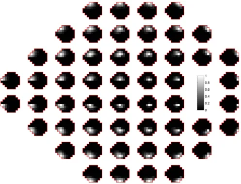
Figure 1c) of the visual field due to the physiological distribution of optic nerve fibres.[23] The unscaled covarianceSbetween each location in the visual field and all other points is illustrated in Figure 2.ANSWERS, in this study, has been specifically adapted to detect deterioration in glaucoma, so the spatial correlationShere encodes the anatomy of optic nerve fibres. To adaptANSWERSfor other types of measurement corresponding to different diseases or conditions,Sshould be adjusted to reflect the characteristics of the spatial correlation present in that data.
The values for the scale parameters a and b were chosen to produce non-informative priors forwaand wb. To be exact, the
slope prior was set asma~0(dB/year) witha~102corresponding
to a slope standard deviation of 10 dB/year. The intercept prior was set such thatmb~18dB(middle of DLS measurement range)
and b~102corresponding to an intercept standard deviation of
10 dB.
According to (6) and (7), the log of posterior probability ofW
lnpðWjY,tÞ~lnX N
i~1
XM j~1
Ryij s wTjti
{1
2ðwa{maÞ T
Laðwa{maÞT
{1
2ðwb{mbÞ T
Lbðwb{mbÞTzconst
ð9Þ
where L{1
a ~aS, L {1
b ~bS. The terms independent of W are
grouped into the constant term,const.
The posterior probability (9) cannot be recognised as a known distribution because (7) is not the conjugate prior of the mixture of
Weibull distributions. Although the log posterior (9) can still be maximised with regard toW, it is difficult to estimate the exact variance of W without knowing the underlying distribution. Therefore, a Laplaceapproximation [31,32] was used to approx-imatepðWjY,tÞas a normal distribution centred at the mode of
W, as described in Appendix S1. The estimates of the slope and intercept in theLaplacemethod exactly match the local maximum
of log posterior probability (9). However, the variance of these slopes and intercepts are approximate estimates.
For the purpose of evaluating the effects of spatial correlation, its contribution can be ‘switched off’ by setting the off-diagonal elements of S in (7) to be 0. This model without spatial enhancement is denoted asANSWER.
ANSWERS indices: identification of change. ANSWERS
estimates the slope wa and intercept wb with their variance
approximated by theLaplacemethod. The distribution of the slope is of particular clinical importance because it represents the rate and certainty of change. The ‘change’ applies equally to deterioration (negative change) and improvement (positive change) in measurements. In the case of a progressive condition, such as glaucoma, the slope distribution at each location can be summarised as the ‘probability of no-deterioration’, which is quantified as the cumulative distribution of slope $0 dB/year. The ‘probability of no-deterioration’ value will be referred to as
Pndhereafter. The Pnd value ranges between 0 and 1 where a lower value indicates a higher probability of deterioration.
In order to summarise the possibility of deterioration across all
M test locations in the visual field series, a global index, the
ANSWERSdeterioration indexI{
[image:6.612.59.557.59.438.2], is defined as:
I{~{X M
j~1
lnPndj ð10Þ
wherePndjis thePndvalue at thejth location in the measurement. I{
is the negative logarithm of the product of allPndvalues, thus, non-negative and larger value implies greater certainty about deterioration in the measurement series. Similarly, to evaluate the improvement in a measurement series, such as in the case of gene therapy for retinal disease,[3] theANSWERSimprovement index
Iz
can be derived asIz~{PM j~1
ln 1{Pndj. However, because
this study illustrates the application on identifying deterioration in retinal function in glaucoma, theANSWERSindex will henceforth only refer toI{
.
Evaluation
To evaluate the utility ofANSWERSin detecting retinal function change, it is necessary to compare it to other change detection methods currently used in clinical decision making. Point-wise linear regression, the most widely used method, fits an ordinary linear regression model to a time series of measurement for each location in the visual field and assesses the significance and slope of the fit. Summary measures, such as the mean deviation from the average DLS of healthy eyes, are also utilised, but since glaucoma tends not to affect all locations to the same extent, global indices often have inadequate statistical sensitivity to detect worsening when compared with methods assessing deterioration at individual locations.[14–17]. Moreover, to evaluate the benefit of taking into account non-stationary variability and spatial correlation respec-tively, ANSWERS without spatial enhancement (ANSWER) was also evaluated. Thus,ANSWERSwas compared with three other methods: ordinary linear regression of mean deviation, point-wise linear regression andANSWER.
Estimation of false positive rates. A false positive is a type I error where change is falsely detected in a series with no true deterioration. The false positive rate can be reliably estimated in a series of repeated measurements acquired in a period of time too short for measureable deterioration. Moreover, randomly reor-dering these repeated measurements produces pseudo-series where there is also no true deterioration.
The series of 12 visual fields from 30 eyes in the test-retest dataset were randomly reordered 300 times, so 90,000 pseudo-series of length between 3 and 12 were generated. It was assumed that one visual field measurement per year was taken in these pseudo series (the median test frequency in the Moorfields dataset). The false positive rate was then estimated as the proportion of series identified as deteriorating. In a clinical situation, false positives may lead to overtreatment and unnecessary cost, so methods with high false positive rates are generally considered as not clinically useful.
Different methods should be compared at equivalent false positive rates, which is dependent on the chosen change criterion and the length of the series. For ordinary linear regression of mean deviation, deterioration criteria were a negative slope andp-value lower than a set threshold. For point-wise linear regression, deterioration criteria for each test location were a negative slope and ap-value,1% and the visual field was worsening when at least n = 1, 2, 3 and 4 contiguous points were deteriorating. For
ANSWERSandANSWER, the criterion for deterioration was aI{
value higher than a given threshold. For each method, a set of
thresholds was chosen to achieve specified false positive rates, and the performance of each method was then compared at equivalent false positive rates.
Time to detect change. The time to detect deterioration was compared between methods using the dataset from electronic health records at Moorfields Eye Hospital. In each visual field series, a subseries containing the first three visual fields was considered as the minimum series length required to detect change. The length of the subseries was then increased by incrementally adding visual fields to the subseries in chronological order. The shortest series that was flagged as deteriorating was then recorded for each method. If no deterioration was detected in any subseries of a visual field series by a method, the time was recoded as the total time span of the series. The comparison among different methods was carried out at equal false positive rates.
Hit rate of change detection. Statistical sensitivity is the measure of a method’s ability to identify true change. Ideally, the sensitivity should be evaluated as the proportion of detected change in the visual field series with true underlying deterioration. However, due to the lack of a ‘gold-standard’ and ‘ground-truth’ classification for glaucomatous deterioration,[33] the underlying worsening status of each visual field series was unknown. Therefore, the methods were compared using the ‘hit rate’, which is the proportion of series flagged as deteriorating in the Moorfields dataset. Given an unknown proportion p% of truly worsening series in the dataset, the hit rate is linked to statistical sensitivity as: hit rate = (p%6sensitivity)+[(12p%)6false positive rate]. Note that if the false positive rate is controlled to be equivalent for all methods, a higher hit rate implies better sensitivity of a method. Therefore, hit rates of all methods were compared as a surrogate comparison for sensitivity.
Results
ANSWERS was implemented in MATLAB R2013a (Math-Works Inc., Natick, MA). Analysis of a series with 10 visual fields took approximately 1.5 seconds on a 2.50 GHz Intel i7 processor. The software is freely available from the authors.
Mixture ofWeibullretest distributions
At all levels of DLS, increasing the number ofWeibullmixture components to be more than 2 does not significantly increase the log likelihood (4) in cross validations. Therefore, two mixture components were used to model retest distribution for sensitivities between 0 dB and 35 dB. The histograms and the derived probability density functions of the Weibull mixture at different DLSs are shown in Figure 3. Despite the non-stationary variability, each distribution can be sufficiently described by a combination of twoWeibulldistributions.
The examples in Figure 4 demonstrate the effect of theWeibull
Time to detect change
Despite the robustness of ANSWER, it does not compromise sensitivity to detect deterioration. In fact, by taking into account the non-stationary variability of DLS measurements, the method is able to detect significant deterioration in short time series where conventional methods cannot reach statistical significance. In Figure 4b, ordinary linear regression did not indicate significant deterioration (p-value.5%), whileANSWERmanaged to ascertain with high certainty that deterioration was occurring (Pnd,0.1%). This property allowsANSWERto provide better time efficiency in detecting deterioration.
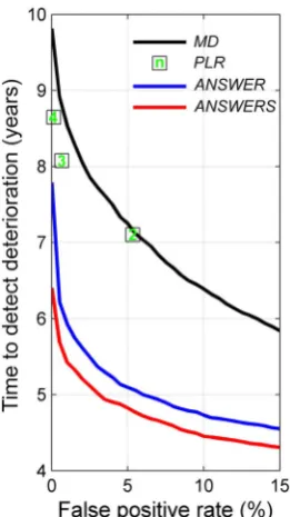
Figure 5 shows the average time to first detect deterioration in the visual field series with each method at false positive rates between 0 and 15% (methods with a higher false positive rate are not clinically useful). Because the criteria for point-wise linear
regression (the number of contiguous points with deterioration in the visual field) are not continuous, the time efficiency of point-wise linear regression could not be estimated with a continuous false positive rate. Moreover, the false positive rate with the single-point criterion of single-point-wise linear regression was higher than 15%, so this was not shown in the figure.
[image:8.612.64.493.58.509.2]For each method, the time to detection change was compared at the 5% false positive rate, or at the closest rate to 5% for point-wise linear regression (two contiguous points, false positive rate of 5.3%). At this false positive rate,ANSWERdetected deterioration faster than point-wise linear regression (p,0.1% paired t-test) and linear regression of mean deviation (p,0.1% paired t-test). Furthermore, with spatial enhancement,ANSWERS was able to detect deterioration significantly faster than ANSWER (p,0.1% paired t-test). On average,ANSWERSdetected deterioration 2.42 (95% confidence interval [2.35, 2.49]) years ahead of point-wise
Figure 3. Histograms of retest differential light sensitivities at levels between 0 dB and 35 dB.The derived probability density function of theWeibullmixture is superimposed in red.
linear regression, 2.28 (95% confidence interval [2.20, 2.35]) years before linear regression of mean deviation, and 0.27 (95% confidence interval [0.22, 0.31]) years beforeANSWER.
Hit rate of change detection
The hit rates of the four methods were estimated with various series lengths and at false positive rates between 0 and 15% using Moorfields dataset. Figure 6 demonstrates the hit rate with series lengths of 5, 7, 9 and 11. Only the hit rates at specified false positive rates between 0 and 15% are displayed (methods with a higher false positive rate are not clinically useful). The areas under the partial hit rate curves for different methods (Figure 6) were compared in Table 1. Because the total area with false positive rate between 0 and 15% is 0.15, the areas under the partial hit rate curves were normalised by being divided by 0.15. Because the hit rate of point-wise linear regression could not be estimated with a continuous false positive rate, the area under the partial hit rate curve was not estimated.
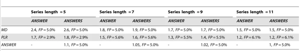
The methods were also compared at the 5% false positive rate, or at the closest rate to 5% for point-wise linear regression (two contiguous points criterion). The ratios of hit rates between pairs of methods are shown in Table 2 where a ratio.1 indicates a better hit rate. For instance, with series of 7 visual fields, the ratio of
ANSWERS against linear regression of mean deviation was 1.9, indicating that the hit rate ofANSWERSis nearly twice that of the latter method.
The hit rates of ANSWER and ANSWERS were higher than linear regression of mean deviation and point-wise linear regression of DLS at all series lengths. There was particular improvement in short series. This explains the better efficiency of
ANSWER and ANSWERS to detect deterioration more quickly. The spatial enhancement included inANSWERSalso increased the hit rate compared with ANSWER, especially with short series. However, this improvement became marginal as the length of series increased.
[image:9.612.60.533.62.291.2]Case studies withANSWERSin comparison with other methods are provided in Appendix S2.
Figure 4. Examples comparingANSWERand ordinary linear regression.The retest distributions of corresponding differential light sensitivity measurements are superimposed as grey areas. The scored probability densities by the ANSWER regression line are marked on the retest distributions.
doi:10.1371/journal.pone.0085654.g004
Figure 5. Time to detect deterioration for linear regression of mean deviation (MD), point-wise linear regression (PLR), ANSWERS andANSWER at false positive rates between 0 and 15%.The number of contiguous points in point-wise linear regression are shown in the square points.
[image:9.612.59.190.431.664.2]Discussion
ANSWERS detected change in retinal function more rapidly than conventional statistical approaches without compromising false positive rates. At equivalent false positive rates, it also detected a greater number of eyes with change in retinal function when compared to the number detected by other widely used methods. TheWeibullmixture retest distributions, in comparison to a normally distributed error assumed in ordinary regression models, allows ANSWERS to attain a high certainty about deterioration status (Figure 4b). In addition, the spatial enhance-ment aggregates information for adjacent locations in the visual field to ‘confirm’ the spatial deterioration pattern, further improving the method especially for short time series. This spatial element of detecting change in visual fields has rarely been considered before.[34–37]ANSWERScould not only aid clinical decision for prompt treatment intervention, but also define more efficient endpoints for clinical trials in eye-related research.[3]
The application and usefulness ofANSWERSin short series is of particular clinical interest. Current widely used methods typified by ordinary linear regression for change detection are limited in short series because they can hardly reach required statistical significance. In clinical situations, where follow-up testing is infrequent, often due to limited resources, these standard analyses
may delay the detection of change in retinal function. In turn this can delay required intensification of treatment. In clinical trials, failing to pick up change in time could also lengthen the trials.
When choosing thresholds forANSWERSto detect deterioration in visual field series, it is critical to consider the false positive rate for the chosen threshold ofI{
. In this study, the threshold was estimated from the test-retest dataset at given false positive rates and for each visual field series length. However, an analytical prescription can be described theoretically and is made available in Appendix S1. Note that I{
threshold does not change with series length given a constant false positive rate.
The Laplacemethod used inANSWERS provides local normal approximation at the mode of the posterior slope and intercept distribution (9), so estimations of variance of these regression parameters may not capture every feature of the distribution (skewness for example). Although the true posterior distribution (9) is unknown, the estimated slope variance from the Laplace
approximation was nonetheless demonstrated to be an effective variable in detecting change and quantifying the certainty about change relative to other current methods.
[image:10.612.60.431.61.293.2]ANSWERSwas developed with the idea that it could be adapted for other applications with similar statistical properties which are not uncommon among other medical and biological measure-ments. For example, serum creatinine measurement for predicting
Figure 6. The hit rates of linear regression of mean deviation (MD), point-wise linear regression (PLR),ANSWERSandANSWERwith series lengths (length) of 5, 7, 9 and 11.The number of contiguous points in point-wise linear regression are shown in the square points. The hit rates are estimated at false positive rates between 0 and 15%.
doi:10.1371/journal.pone.0085654.g006
Table 1.The normalised areas under partial hit rate curves forANSWER,ANSWERS, linear regression of mean deviation (MD).
Series length = 5 Series length = 7 Series length = 9 Series length = 11
ANSWER 0.39 0.48 0.55 0.62
ANSWERS 0.41 0.49 0.56 0.62
MD 0.20 0.29 0.35 0.44
[image:10.612.59.556.642.711.2]kidney failure,[38] heart rate measurement for assessing heart attack risk [39] and baroreceptor sensitivity feedback in diabetes mellitus [40] pose similar challenges in clinical decision making. There are two necessary steps in order to adapt ANSWERSfor application to other types of clinical measurements. First, the non-stationary variability should be derived from the measurement in question. Since the Weibullmixture distribution is versatile and concise, it could easily be adjusted to model other retest distributions using the expectation-maximisation algorithm pre-sented in Appendix S1. Second, the current spatial correlation (8) stems from the anatomy of retinal nerve fibres and therefore is not directly applicable to measurements and conditions other than optic neuropathies. Thus, the spatial correlation in (8) would need to be adapted (or removed if necessary) to reflect the spatial characteristics of the measurement or disease process in question. Moreover, ANSWERS was used to infer linear change because there are generally insufficient data to identify non-linear change due to the short visual field series in clinical practice; however, configuringANSWERSto measure change of conditions with long series and temporal processes showing non-linear change is trivial, and can be done by changing the time vectortiin (6) to nonlinear
components such as radial basis functions.
In this study, test-retest data were used to estimate variability and false positive rates. Due to the lack of gold standard about deterioration in retinal function, these data were acquired within a very short period of time (12 visual fields in less than 8 weeks) so it is highly unlikely that measurable damage occurred in this period. However, the patients that make up this dataset may gain psychophysical experience quicker than general clinic patients who typically undertake perimetry tests much less frequently. Therefore patients in the test-retest data could produce measurements with lower variability than that observed in clinical practice. However, all methods were evaluated using the same test-retest data, hence the false positive rates would be equivalently underestimated for each technique. Therefore, despite the potential to underestimate variability, test-retest data does allow us to makes a fair comparison among the methods evaluated.
It is important to note that despite the evolution of new statistical methods for analysing change in retinal function, improving data acquisition techniques should continue to be at the forefront of research. Producing less variable data at the point of measurement acquisition will allow more accurate change detection. Studies have already demonstrated various approaches
to improve measurements of DLS. Examples include, but are not limited to, modulation in stimulus size,[41,42] testing in a linear scale rather than a log scale [43] and increasing the density or changing spatial arrangement of test points.[44,45] It was also reported that DLS less than 15 dB is not associated with the loss of ganglion cells and may not contain significant information about the integrity of retinal function.[46] Therefore, there is a real need to accurately measure changes in DLS sooner while it exceeds 15 dB.
In conclusion,ANSWERSprovides a solution in a landscape of uncertainty in detecting retinal function deterioration. This could, for example, impact on how patients with glaucoma are monitored and treated and the efficiency and duration of clinical trials.
ANSWERS was shown to outperform conventional methods of detecting retinal function deterioration both in terms of statistical sensitivity, and in time taken to detect change. ANSWERS was demonstrated to detect visual field deterioration caused by glaucoma, but there is plenty of scope for its use in other measurements subject to non-stationary variability and spatial correlation.
Supporting Information
Appendix S1 Detailed mathematical derivation. Expec-tation-maximisation algorithm for Weibull mixture distribution, Laplace approximation forANSWERSand an analytical model for calculating ANSWERS threshold given false positive rates and series lengths.
(PDF)
Appendix S2 Examples illustrating ANSWERS in com-parison with other methods under study.
(PDF)
Acknowledgments
We thank Dr. Paul H Artes from Ophthalmology and Visual Sciences, Dalhousie University, Halifax, Nova Scotia, Canada, for organising and transferring the test-retest dataset.
Author Contributions
Conceived and designed the experiments: HZ DGH DC RR. Performed the experiments: HZ LS SC DGH. Analyzed the data: HZ RR LS SC DC. Wrote the paper: HZ RR LS SC DGH DC.
References
1. Morgan JE (2012) Retina ganglion cell degeneration in glaucoma: an opportunity missed? A review. Clin Experiment Ophthalmol 40: 364–368.
[image:11.612.62.556.90.175.2]2. Patel PJ, Chen FK, Da Cruz L, Rubin GS, Tufail A (2011) Contrast sensitivity outcomes in the ABC Trial: a randomized trial of bevacizumab for neovascular age-related macular degeneration. Invest Ophthalmol Vis Sci 52: 3089–3093. Table 2.The ratio of the hit rates forANSWERandANSWERS(in columns) against those of linear regression of mean deviation (MD), point-wise linear regression (PLR) of differential light sensitivity andANSWER(in rows).
Series length = 5 Series length = 7 Series length = 9 Series length = 11
ANSWER ANSWERS ANSWER ANSWERS ANSWER ANSWERS ANSWER ANSWERS
MD 2.4,FP= 5.0% 2.6,FP= 5.0% 1.8,FP= 5.0% 1.9,FP= 5.0% 1.7,FP= 5.0% 1.7,FP= 5.0% 1.5,FP= 5.0% 1.5,FP= 5.0%
PLR 1.7,FP= 2.9% 1.8,FP= 2.9% 1.5,FP= 5.6% 1.6,FP= 5.6% 1.3,FP= 5.5% 1.4,FP= 5.5% 1.2,FP= 6.1% 1.2,FP= 6.1%
ANSWER - 1.1,FP= 5.0% - 1.05,FP= 5.0% - 1.02,FP= 5.0% - 1,FP= 5.0%
The false positive rate (FP) at which the ratio was estimated is also given. The ratio is calculated for criteria giving 5% false positive rates, or at a false positive rate closest to 5% for point-wise linear regression where the false positive rate cannot be continuously estimated. The comparison was carried out with series lengths of 5, 7, 9 and 11.
3. Bainbridge JW, Smith AJ, Barker SS, Robbie S, Henderson R, et al. (2008) Effect of gene therapy on visual function in Leber’s congenital amaurosis. N Engl J Med 358: 2231–2239.
4. Cramer AO, Maclaren RE (2013) Translating induced pluripotent stem cells from bench to bedside: application to retinal diseases. Curr Gene Ther 13: 139– 151.
5. Guo L, Duggan J, Cordeiro MF (2010) Alzheimer’s disease and retinal neurodegeneration. Curr Alzheimer Res 7: 3–14.
6. Koronyo-Hamaoui M, Koronyo Y, Ljubimov AV, Miller CA, Ko MK, et al. (2011) Identification of amyloid plaques in retinas from Alzheimer’s patients and noninvasive in vivo optical imaging of retinal plaques in a mouse model. Neuroimage 54: S204–217.
7. Oliveira C, Cestari DM, Rizzo JF (2012) The use of fourth-generation optical coherence tomography in multiple sclerosis: a review. Semin Ophthalmol 27: 187–191.
8. Trip SA, Schlottmann PG, Jones SJ, Altmann DR, Garway-Heath DF, et al. (2005) Retinal nerve fiber layer axonal loss and visual dysfunction in optic neuritis. Ann Neurol 58: 383–391.
9. McNeill A, Roberti G, Lascaratos G, Hughes D, Mehta A, et al. (2013) Retinal thinning in Gaucher disease patients and carriers: Results of a pilot study. Mol Genet Metab 109: 221–223.
10. Quigley HA, Broman AT (2006) The number of people with glaucoma worldwide in 2010 and 2020. British Journal of Ophthalmology 90: 262–267. 11. Pizzarello L, Abiose A, Ffytche T, Duerksen R, Thulasiraj R, et al. (2004)
VISION 2020: The Right to Sight: a global initiative to eliminate avoidable blindness. Arch Ophthalmol 122: 615–620.
12. Viswanathan AC, Crabb DP, McNaught AI, Westcott MC, Kamal D, et al. (2003) Interobserver agreement on visual field progression in glaucoma: a comparison of methods. Br J Ophthalmol 87: 726–730.
13. Tanna AP, Bandi JR, Budenz DL, Feuer WJ, Feldman RM, et al. (2011) Interobserver agreement and intraobserver reproducibility of the subjective determination of glaucomatous visual field progression. Ophthalmology 118: 60–65.
14. Katz J, Gilbert D, Quigley HA, Sommer A (1997) Estimating progression of visual field loss in glaucoma. Ophthalmology 104: 1017–1025.
15. Smith SD, Katz J, Quigley HA (1996) Analysis of progressive change in automated visual fields in glaucoma. Invest Ophthalmol Vis Sci 37: 1419–1428. 16. Birch MK, Wishart PK, O’Donnell NP (1995) Determining progressive visual field loss in serial Humphrey visual fields. Ophthalmology 102: 1227-1234; discussion 1234–1225.
17. Chauhan BC, Drance SM, Douglas GR (1990) The use of visual field indices in detecting changes in the visual field in glaucoma. Invest Ophthalmol Vis Sci 31: 512–520.
18. Heijl A, Leske MC, Bengtsson B, Hussein M (2003) Measuring visual field progression in the Early Manifest Glaucoma Trial. Acta Ophthalmol Scand 81: 286–293.
19. Artes PH (2008) Progression: things we need to remember but often forget to think about. Optom Vis Sci 85: 380–385.
20. Artes PH, Iwase A, Ohno Y, Kitazawa Y, Chauhan BC (2002) Properties of perimetric threshold estimates from Full Threshold, SITA Standard, and SITA Fast strategies. Invest Ophthalmol Vis Sci 43: 2654–2659.
21. Henson DB, Chaudry S, Artes PH, Faragher EB, Ansons A (2000) Response Variability in the Visual Field: Comparison of Optic Neuritis, Glaucoma, Ocular Hypertension, and Normal Eyes Invest Ophthalmol Vis Sci 41: 417–421. 22. Russell RA, Crabb DP, Malik R, Garway-Heath DF (2012) The relationship
between variability and sensitivity in large-scale longitudinal visual field data. Invest Ophthalmol Vis Sci 53: 5985–5990.
23. Garway-Heath DF, Poinoosawmy D, Fitzke FW, Hitchings RA (2000) Mapping the visual field to the optic disc in normal tension glaucoma eyes. Ophthalmology 107: 1809–1815.
24. Strouthidis NG, Vinciotti V, Tucker AJ, Gardiner SK, Crabb DP, et al. (2006) Structure and Function in Glaucoma: The Relationship between a Functional
Visual Field Map and an Anatomic Retinal Map. Investigative Ophthalmology & Visual Science 47: 5356–5362.
25. Chauhan BC, Garway-Heath DF, Gon˜i FJ, Rossetti L, Bengtsson B, et al. (2008) Practical recommendations for measuring rates of visual field change in glaucoma. British Journal of Ophthalmology 92: 569–573.
26. Heijl A, Lindgren G, Olsson J (1989) The effect of perimetric experience in normal subjects. Arch Ophthalmol 107: 81–86.
27. Wild JM, Dengler-Harles M, Searle AE, O’Neill EC, Crews SJ (1989) The influence of the learning effect on automated perimetry in patients with suspected glaucoma. Acta Ophthalmol (Copenh) 67: 537–545.
28. Patterson AJ, Garway-Heath DF, Strouthidis NG, Crabb DP (2005) A New Statistical Approach for Quantifying Change in Series of Retinal and Optic Nerve Head Topography Images. Investigative Ophthalmology & Visual Science 46: 1659–1667.
29. Frackowiak RSJ (1997) Human Brain Function: Academic Press San Diego. 30. Dempster A, Laird N, Rubin D (1977) Maximum likelihood from incomplete
data via the EM algorithm. Journal of the Royal Statistical Society 39(1): 1–38. 31. Tierney L, Kadane J (1986) Accurate approximations for posterior moments and marginal densities. Journal of the American Statistical Association 81: 82–86. 32. Bishop CM (1996) Neural network for pattern recognition. New York: Oxford
University Press.
33. Gardiner SK, Crabb DP (2002) Examination of different pointwise linear regression methods for determining visual field progression. Invest Ophthalmol Vis Sci 43: 1400–1407.
34. Crabb DP, Fitzke FW, McNaught AI, Edgar DF, Hitchings RA (1997) Improving the prediction of visual field progression in glaucoma using spatial processing. Ophthalmology 104: 517–524.
35. Swift S, Liu X (2002) Predicting glaucomatous visual field deterioration through short multivariate time series modelling. Artif Intell Med 24: 5–24.
36. Strouthidis NG, Scott A, Viswanathan AC, Crabb DP, Garway-Heath DF (2007) Monitoring glaucomatous visual field progression: the effect of a novel spatial filter. Invest Ophthalmol Vis Sci 48: 251–257.
37. Tucker A, Vinciotti V, Liu X, Garway-Heath D (2005) A spatio-temporal Bayesian network classifier for understanding visual field deterioration. Artif Intell Med 34: 163–177.
38. Turin TC, Hemmelgarn BR (2011) Change in kidney function over time and risk for adverse outcomes: is an increasing estimated GFR harmful? Clin J Am Soc Nephrol 6: 1805–1806.
39. Rajendra Acharya U, Paul Joseph K, Kannathal N, Lim CM, Suri JS (2006) Heart rate variability: a review. Med Biol Eng Comput 44: 1031–1051. 40. Bogachev MI, Mamontov OV, Konradi AO, Uljanitski YD, Kantelhardt JW, et
al. (2009) Analysis of blood pressure-heart rate feedback regulation under non-stationary conditions: beyond baroreflex sensitivity. Physiol Meas 30: 631–645. 41. Redmond T, Garway-Heath DF, Zlatkova MB, Anderson RS (2010) Sensitivity loss in early glaucoma can be mapped to an enlargement of the area of complete spatial summation. Invest Ophthalmol Vis Sci 51: 6540–6548.
42. Swanson WH, Felius J, Birch DG (2000) Effect of stimulus size on static visual fields in patients with retinitis pigmentosa. Ophthalmology 107: 1950–1954. 43. Malik R, Swanson WH, Garway-Heath DF (2006) Development and evaluation
of a linear staircase strategy for the measurement of perimetric sensitivity. Vision Res 46: 2956–2967.
44. Westcott MC, Garway-Heath DF, Fitzke FW, Kamal D, Hitchings RA (2002) Use of high spatial resolution perimetry to identify scotomata not apparent with conventional perimetry in the nasal field of glaucomatous subjects. British Journal of Ophthalmology 86: 761–766.
45. Asaoka R, Russell RA, Malik R, Crabb DP, Garway-Heath DF (2012) A novel distribution of visual field test points to improve the correlation between structure-function measurements. Invest Ophthalmol Vis Sci 53: 8396–8404. 46. Harwerth RS, Carter-Dawson L, Shen F, Smith EL 3rd, Crawford ML (1999)