Exact dynamic stiffness elements based on one-dimensional higher-order theories for free vibration analysis of solid and thin-walled structures

      

City, University of London Institutional Repository

Citation:

Pagani, A., Boscolo, M., Banerjee, J. R. and Carrera, E. (2013). Exact dynamic stiffness elements based on one-dimensional higher-order theories for free vibration analysis of solid and thin-walled structures. Journal of Sound and Vibration, 332(23), pp. 6104-6127. doi: 10.1016/j.jsv.2013.06.023

This is the accepted version of the paper.

This version of the publication may differ from the final published

version.

Permanent repository link:

http://openaccess.city.ac.uk/14991/

Link to published version:

http://dx.doi.org/10.1016/j.jsv.2013.06.023

Copyright and reuse: City Research Online aims to make research

outputs of City, University of London available to a wider audience.

Copyright and Moral Rights remain with the author(s) and/or copyright

holders. URLs from City Research Online may be freely distributed and

linked to.

Exact Dynamic Stiffness Elements based on One-Dimensional

Higher-Order Theories for Free Vibration Analysis of Solid and

Thin-Walled Structures

A. Pagania∗_{, M. Boscolo}b†_{, J. R. Banerjee}b‡_{, and E. Carrera}a§

a_{Department of Mechanical and Aerospace Engineering, Politecnico di Torino,} Corso Duca degli Abruzzi 24, 10129 Torino, Italy.

b _{School of Engineering and Mathematical Sciences, City University London,} Northampton Square, London, EC1V 0HB, United Kingdom.

Submitted to:

Journal of Sound and Vibration

Author for correspondence:

A. Pagani, Ph.D. Student,

Department of Mechanical and Aerospace Engineering, Politecnico di Torino,

Corso Duca degli Abruzzi 24, 10129 Torino, Italy,

tel: +39 011 090 6870, fax: +39 011 090 6899,

e-mail: [email protected]

∗_{Ph.D. Student, e-mail: [email protected]} †_{Researcher Fellow, e-mail: [email protected]}

‡_{Professor of Aeronautical Engineering, e-mail: [email protected]}

Abstract

In this paper, an exact dynamic stiffness formulation using one-dimensional (1D) higher-order the-ories is presented and subsequently used to investigate the free vibration characteristics of solid and thin-walled structures. Higher-order kinematic fields are developed using the Carrera Unified Formu-lation, which allows for straightforward implementation of any-order theories without the need for ad hoc formulations. Classical beam theories (Euler-Bernoulli and Timoshenko) are also captured from the formulation as degenerate cases. The Principle of Virtual Displacements is used to derive the governing differential equations and the associated natural boundary conditions. An exact dynamic stiffness matrix is then developed by relating the amplitudes of harmonically varying loads to those of the responses. The explicit terms of the dynamic stiffness matrices are also presented. The result-ing dynamic stiffness matrix is used with particular reference to the Wittrick-Williams algorithm to carry out the free vibration analysis of solid and thin-walled structures. The accuracy of the theory is confirmed both by published literature and by extensive finite element solutions using the commercial code MSC/NASTRANR_.

Keywords: Dynamic stiffness method; Unified formulation; Free vibration; Higher-order theories;

1

Introduction

Beam models are widely used to analyze the mechanical behavior of slender bodies, such as columns,

rotor-blades, aircraft wings, towers, antennae and bridges amongst others. The simplicity of 1D

theories and their ease of application coupled with computational efficiency are some of the main

reasons why structural analysts prefer them to two-dimensional (2D) and three-dimensional (3D)

models.

The classical and best-known beam theories that survived the test of time and still valid to this

day, are those by Euler [1] - hereinafter referred to as EBBM - and Timoshenko [2, 3] - hereinafter

referred to as TBM. The former does not account for transverse shear deformations and rotatory

inertia, whereas the latter assumes a uniform shear distribution along the cross-section of the beam

together with the effects of rotatory inertia. These models yield reasonably good results when

slender, solid section, homogeneous structures are subjected to flexure. Conversely, the analysis of

deep, thin-walled, open section beams may require more sophisticated theories to achieve sufficiently

accurate results, see [4].

Over the last century, many refined beam theories have been proposed to overcome the limitation

of classical beam modelling. Different approaches have been used to improve the beam models, which

include the introduction of shear correction factors, the use of warping functions based on de

Saint-Venant’s solution, the variational asymptotic solution (VABS), the generalized beam theory (GBT),

and others. Some selective references and noteworthy contributions are briefly discussed below, with

particular attention to dynamic analysis which is the main focus of this paper.

Early investigators have focused on the use of appropriate shear corrections factors to increase

the accuracy of classical 1D formulations, see for examples Timoshenko and Goodier [5], Sokolniko

[6], Stephen [7], and Hutchinson [8]. The shear correction factor has generally been used as a static

concept which is restrictive. In this respect, Jensen [9] showed how the shear correction factor can

vary with the natural frequencies. Furthermore, a review paper by Kaneko [10] and a recent paper

by Dong et al. [11] highlighted the difficulty in the definition of a universally accepted formulation

for shear correction factors.

Another important class of refinement methods reported in the literature is based on the use of

warping functions. The contributions by El Fatmi [12, 13, 14] and Ladev´eze et al. [15, 16] are some

excellent examples. Rand [17] and Kim and White [18] used more or less the same approach in the

Asymptotic type expansion in conjunction with variational methods has also been proposed

particularly by Berdichevsky et al. [19], in which a commendable review of previous works on beam

theory developments is given. Some further valuable contributions are by Volovoi [20], Popescu and

Hodges [21], Yu et al. [22], Yu and Hodges [23, 24]. Other related work can be found in the papers

published by Kim and Wang [25] and Firouz-Abad et al. [26].

The generalized beam theory (GBT) probably was originated from the work of Schardt [27, 28].

GBT improves classical theories by using piece-wise beam description of thin-walled sections. It has

been widely employed and extended in various forms by Silvetre et al. [29, 30, 31] and a dynamic

application has been presented by Bebiano et al. [32].

Higher-order theories are generally obtained by using refined displacement fields of the beam

cross-sections. Washizu [33] ascertained how the use of an arbitrarily chosen rich displacement

fields can lead to closed form exact 3D solutions. Many other higher-order theories have also been

introduced to include non-classical effects. A review was compiled by Kapania and Raciti [34, 35]

focusing on flexural deformation, vibration analysis, wave propagations, buckling and post-buckling

behaviour.

The present work is focused on 1D higher-order theories based on generalized displacement

variables to carry out free vibration analysis of solid and thin-walled structures. Refined beam

models are developed within the framework of Carrera Unified Formulation (CUF) which is well

established in the literature for over a decade [36, 37, 38, 39, 40]. CUF is a hierarchical formulation

that considers the order of the model, N, as a free-parameter (i.e. as an input) of the analysis or

in other words, refined models are obtained without having the need for any ad hoc formulations.

In the present work, beam theories using CUF are obtained on the basis of Taylor-type expansions

(TE). EBBM and TBM can be obtained as particular or special cases. The strength of CUF TE 1D

models in dealing with arbitrary geometries, thin-walled structures and identifying local effects are

well known for both static [41, 42] and free-vibration analysis [43, 44, 45].

In majority of the papers on 1D CUF, the finite element method (FEM) has been used to handle

arbitrary geometries and loading conditions. The present work is intended to provide a more powerful

approach for CUF TE theories through the application of the dynamic stiffness method (DSM) to

carry out the free vibration analysis of solid and thin-walled structures in a much broader context

by allowing for the cross-sectional deformation. DSM has been quite extensively developed for beam

elements by Banerjee [46, 47, 48, 49, 50], Banerjee et al. [51], and Williams and Wittrick [52]. Plate

Recently, DSM has been applied to Mindlin plate assemblies by Boscolo and Banerjee in [55, 56],

where a more comprehensive review on the use of DSM can be found.

The DSM is appealing in dynamic analysis because unlike the FEM, it provides exact solution

of the equations of motion of a structure once the initial assumptions on the displacements field

have been made. This essentially means that, unlike the FEM and other approximate methods,

the model accuracy is not unduly compromised when a small number of elements are used in the

analysis. For instance, one single structural element can be used in the DSM to compute any number

of natural frequencies to any desired accuracy. Of course, the accuracy of the DSM will be as good

as the accuracy of the governing differential equations of the structural element in free vibration. In

fact, the exact dynamic stiffness (DS) matrix stems from the solution of the governing differential

equations.

In this work, CUF is adopted to automatically build any-order beam theory which is the

funda-mental prerequisite to develop 1D higher-order exact DS elements as the objective. The investigation

is carried out in the following steps: (i) first CUF is introduced and higher-order models are

formu-lated, (ii) secondly, the Principle of Virtual Displacements (PVD) is used to derive the differential

governing equations and the associated natural boundary conditions for the generic N-order model,

(iii) next, by assuming harmonic oscillation, the equilibrium equations and the natural boundary

conditions are formulated in the frequency domain by making extensive use of symbolic computation,

(iv) the resulting system of ordinary differential equations of second order with constant coefficients

is then solved in closed analytical form, (v) subsequently, the frequency dependent DS matrix of the

system is derived by relating the amplitudes of the harmonically varying nodal generalised forces to

those of the nodal generalized displacements, and (vi) finally, the well-known algorithm of Wittrick

and Williams [57] is applied to the resulting DS matrix for free vibration analysis of compact and

thin-walled structures.

2

1D unified formulation

2.1 Preliminaries

The adopted rectangular cartesian coordinate system is shown in Fig. 1. Let us introduce the

transposed displacement vector,

u(x, y, z;t) =

ux uy uz

T

The cross-sectional plane of the structure is denoted by Ω, and the beam boundaries over y are

0≤y≤L. The stress, σ_{, and strain,}ǫ_{, components are grouped as follows:}

σ_{p =}

σzz σxx σzx

T

, ǫ_{p =}

ǫzz ǫxx ǫzx

T

σ_n=

σzy σxy σyy

T

, ǫ_n=

ǫzy ǫxy ǫyy

T (2)

In the case of small displacements with respect to a characteristic dimension in the plane of Ω, the

strain - displacement relations are

ǫ_{p =Dpu}

ǫ_{n=Dnu= (DnΩ+Dny)u}

(3)

where Dp and Dn are linear differential operators and the subscript “n” stands for terms lying on

the cross-section, while “p” stands for terms lying on planes which are orthogonal to Ω.

Dp =

      

0 0 ∂

∂z ∂

∂x 0 0

∂ ∂z 0 ∂ ∂x       

, DnΩ=

       0 ∂ ∂z 0

0 _∂x∂ 0

0 0 0

      

, Dny =

      

0 0 ∂

∂y ∂

∂y 0 0

0 _∂y∂ 0

       (4)

Constitutive laws are now exploited to obtain stress components to give

σ_=C˜ǫ ₍₅₎

Equation (5) can be split into ǫ_{p and} ǫ_{nwith the help of Eq. (2) so that}

σ_{p =C}˜_ppǫ_p+C˜_pnǫ_n

σ_n=C˜_npǫ_p+C˜_nnǫ_n

(6)

In the case of orthotropic material the matrices C˜pp,C˜nn,C˜pn, and C˜np are

˜ Cpp=

      ˜

C11 C˜12 0

˜

C12 C˜22 0

0 0 C˜44

     

, C˜nn =

      ˜

C55 0 0

0 C˜66 C˜36

0 C˜36 C˜33

     

, C˜pn =C˜ T np=      

0 C˜16 C˜13

0 C˜26 C˜23

˜

C45 0 0

Coefficients ˜Cij depend on the Young’s modulus, Poisson’s ratio, and fiber orientation angle. For

the sake of brevity, the expressions for the coefficients ˜Cij are not reported here, but can be found

in standard texts, see for example Tsai [58] and Reddy [59]. In the present paper the governing

equations are derived for the generic case of orthotropic material. However, applications to metallic

isotropic structures will be shown.

Within the framework of the CUF, the displacement fieldu(x, y, z;t) can be expressed as

u(x, y, z;t) =Fτ(x, z)uτ(y;t), τ = 1,2, ...., M (8)

where Fτ are the functions of the coordinates x and z on the cross-section. uτ is the vector of

the generalized displacements, M stands for the number of terms used in the expansion, and the repeated subscript, τ, indicates summation. The choice of Fτ determines the class of the 1D CUF

model that is required and subsequently to be adopted. TE (Taylor expansion) 1D CUF models

-described by Eq. (8) - consists of a Maclaurin series that uses the 2D polynomials xi zj as base,

where i and j are positive integers. Table 1 shows M and Fτ as functions of the expansion order,

N. For instance, the displacement field of the second-order (N = 2) TE model can be expressed as

ux=ux1 +x ux2 +z ux3+x2 ux4 +xz ux5+z2 ux6

uy =uy1+x uy2+z uy3 +x2uy4 +xz uy5+z2 uy6

uz=uz1 +x uz2 +z uz3 +x2uz4+xz uz5 +z2 uz6

(9)

The orderN of the expansion is set as an input option of the analysis; the integerN is arbitrary and

defines the order the beam theory. The Timoshenko beam model (TBM) can be realised by using a

suitableFτ expansion. Two conditions have to be imposed: (1) a first-order (N = 1) approximation

kinematic field:

ux =ux1+x ux2 +z ux3

uy =uy1 +x uy2 +z uy3

uz =uz1 +x uz2 +z uz3

(10)

(2) the displacement components ux anduz have to be constant above the cross-section:

ux2 =uz2 =ux3 =uz3 = 0 (11)

By contrast, the Euler-Bernoulli beam model (EBBM) can be obtained through the penalization of

to give

σxy =χC˜55ǫxy+χC˜45ǫzy

σzy=χC˜45ǫxy +χC˜55ǫxy

(12)

Classical theories and first-order models (N = 1) require the necessary assumption of reduced

material stiffness coefficients to correct Poisson’s locking (see [39]). In this paper, Poisson’s locking

is corrected according to the method outlined by Carrera et al. [40].

2.2 Governing equations of the N-order TE model

The principle of virtual displacements is used to derive the equations of motion.

δLint =

Z

V

(δǫT_pσ_p+δǫT_nσ_{n) dV =−δLine (13)}

whereLintstands for the strain energy andδLine is the work done by the inertial loadings. δ stands

for the usual virtual variation operator. The virtual variation of the strain energy is rewritten using

Eq.s (3), (6) and (8). After integrations by part, Eq. (13) becomes

δLint=

Z

L

δuTτKτ susdy+

h

δuTτΠτ sus

iy=L

y=0 (14)

where Kτ s is the differential linear stiffness matrix and Πτ s is the matrix of the natural boundary

conditions in the form of 3_×3 fundamental nuclei. The components ofKτ s are provided as follows

and they are referred to as Kτ s

number (j = 1,2,3)

K₍₁₁₎τ s =Eτ,22xs,x+E

44

τ,zs,z + E

26

τ,xs−E

26

τ s,x

∂

∂y −E

66

τ s

∂2

∂y2

K₍₁₂₎τ s =Eτ,26xs,x+E

45

τ,zs,z + E

23

τ,xs−E

66

τ s,x

∂

∂y −E

36

τ s

∂2 ∂y2

Kτ s

(13) =Eτ,12xs,z +E

44

τ,zs,x+ E

45

τ,zs−E

16

τ s,z

∂

∂y

Kτ s

(21) =Eτ,26xs,x+E

45

τ,zs,z + E

66

τ,xs−E

23

τ s,x

∂

∂y −E

36

τ s

∂2 ∂y2

Kτ s

(22) =Eτ,66xs,x+E

55

τ,zs,z + E

36

τ,xs−E

36

τ s,x

∂

∂y −E

33

τ s

∂2

∂y2

Kτ s

(23) =Eτ,16xs,z +E

45

τ,zs,x+ E

55

τ,zs−E

13

τ s,z

∂

∂y Kτ s

(31) =Eτ,44xs,z +E

12

τ,zs,x+ E

16

τ,zs−E

45

τ s,z

∂

∂y

K₍₃₂₎τ s =Eτ,45xs,z +E

16

τ,zs,x+ E

13

τ,zs−E

55

τ s,z

∂

∂y

K₍₃₃₎τ s =Eτ,44xs,x+E

11

τ,zs,z + E

45

τ,xs−E

45

τ s,x

∂

∂y −E

55

τ s

∂2 ∂y2

(15)

The generic term Eτ,αβθs,ζ above is a cross-sectional moment parameter

E_τ,αβ_θs,ζ =

Z

Ω

˜

CαβFτ,θFs,ζdΩ (16)

The suffix after the comma in Eq. (15) denotes the derivatives. As far as the boundary conditions

are concerned, the components of Πτ s are

Πτ s₍₁₁₎ =Eτ s,26x+E

66

τ s

∂ ∂y, Π

τ s

(12)=Eτ s,66x +E

36

τ s

∂ ∂y, Π

τ s

(13) =Eτ s16

Πτ s

(21) =Eτ s,23x+E

36

τ s

∂ ∂y, Π

τ s

(22)=Eτ s,36x +E

33

τ s

∂ ∂y, Π

τ s

(23) =Eτ s,13z

Πτ s

(31) =Eτ s45, Πτ s(32)=Eτ s,55z, Π

τ s

(33) =Eτ s,45x+E

55

τ s

∂ ∂y

(17)

The virtual variation of the inertial work is given by

δLine=

Z

L

δuτ

Z

Ω

ρFτFsdΩ ¨usdy=

Z

L

The explicit form of the governing equations is

δuxτ : −Eτ s66uxs,yy+ E

26

τ,xs−E

26

τ s,x

uxs,y+ E

22

τ,xs,x +E

44

τ,zs,z

uxs

−Eτ s36uys,yy+ E

23

τ,xs−E

66

τ s,x

uys,y+ E

26

τ,xs,x +E

45

τ,zs,z

uys

+ E45

τ,zs−E

16

τ s,z

uzs,y+ Eτ,44zs,x+E

12

τ,xs,z

uzs=−Eρτ su¨xs

δuyτ : −Eτ s36uxs,yy+ E66τ,xs−E

23

τ s,x

uxs,y+ Eτ,26xs,x +E

45

τ,zs,z

uxs

−E_{τ s}33uys,yy+ E

36

τ,xs−E

36

τ s,x

uys,y+ E

66

τ,xs,x +E

55

τ,zs,z

uys

+ E_τ,55_zs−E_{τ s,}13_z

uzs,y+ Eτ,16xs,z +E

45

τ,zs,x

uzs=−Eρτ su¨ys

δuzτ : Eτ,16zs−E

45

τ s,z

uxs,y+ Eτ,44xs,z +E

12

τ,zs,x

uxs

+ E13

τ,zs−E

55

τ s,z

uys,y+ Eτ,45xs,z +E

16

τ,zs,x

uys−E55τ suzs,yy

+ E45

τ,xs−E

45

τ s,x

uzs,y+ Eτ,44xs,x+E

11

τ,zs,z

uzs =−Eτ sρu¨zs

(19)

where

E_{τ s}ρ =

Z

Ω

ρFτFsdΩ (20)

Double over dots stand as second derivative with respect to time (t). LettingPτ =

Pxτ Pyτ Pzτ

T

to be the vector of the generalized forces, the natural boundary conditions are

δuxτ : Pxs=E66τ suxs,y+E26τ s,xuxs+E

36

τ suys,y+Eτ s,66xuys+E

16

τ s,zuzs

δuyτ : Pys=Eτ s36uxs,y+Eτ s,23xuxs+E

33

τ suys,y+Eτ s,36xuys+E

13

τ s,zuzs

δuzτ : Pzs =Eτ s,45zuxs+E

55

τ s,zuys+E

55

τ suzs,y+Eτ s,45xuzs

(21)

For a fixed approximation orderN, Eq.s (19) and (21) have to be expanded using the indices τ and

desired model. The equations for classical TBM and EBBM could also be obtained from Eq.s (19)

and (21). For instance, the governing equations of TBM can be found from Eq. (19) by expanding

the terms ux1,uy1,uz1 (i.e. the translational displacements of the beam axis) and uy2,uy3 (i.e. the

rotations of the cross-section about the z- and x-axis). Similarily EBBM could also be captured from

TBM formulation by choosing a proper combination of Fτ in order to write the rotations unknowns

(i.e. uy2,uy3) as functions of the cross-sectional displacementsux1 anduz1. However, in the present

paper, EBBM is straightforwardly obtained from TBM by penalizing the shear stiffness as discussed

in Section 2.1.

In the case of harmonic motion, the solution of Eq.s (19) is sought in the form

us(y;t) =Us(y) eiωt (22)

whereUs(y) is the amplitude function of the motion,ωis an arbitrary circular or angular frequency,

and i is √−1. Equations (22) allows the formulation of the equilibrium equations and the natural

boundary conditions in the frequency domain. Substituting Eq. (22) into Eq.s (19), a set of three

coupled ordinary differential equations is obtained which can be written in a matrix form as follows:

δUτ : Lτ sU˜s= 0 (23)

where

˜

Us=

Uxs Uxs,y Uxs,yy Uys Uys,y Uys,yy Uzs Uzs,y Uzs,yy

T

(24)

and Lτ s is the 3_×9 fundamental nucleus which contains the coefficients of the ordinary differential

equations. The components of matrixLτ sare provided below and they are referred to asLτ s

iis the row number (i= 1,2,3) andj is the column number (j = 1,2, ...,9)

Lτ s

(11) =−ω2E

ρ

τ s+Eτ,22xs,x+E

44

τ,zs,z, L

τ s

(12) =Eτ,26xs−E

26

τ s,x, L

τ s

(13) =−Eτ s66

Lτ s₍₁₄₎ =Eτ,26xs,x +E

45

τ,zs,z, L

τ s

(15) =Eτ s,23x−E

66

τ s,x, L

τ s

(16) =−Eτ s36

Lτ s

(17) =Eτ,12xs,z +E

44

τ,zs,x, L

τ s

(18) =Eτ,45zs−E

16

τ s,z, L

τ s

(19) = 0

Lτ s

(21) =Eτ,26xs,x +E

45

τ,zs,z, L

τ s

(22) =Eτ,66xs−E

23

τ s,x, L

τ s

(23) =−Eτ s36

Lτ s

(24) =−ω2E

ρ

τ s+Eτ,66xs,x+E

55

τ,zs,z, L

τ s

(25) =Eτ,36xs−E

36

τ s,x, L

τ s

(26) =−Eτ s33

Lτ s₍₂₇₎ =Eτ,16xs,z +E

45

τ,zs,x, L

τ s

(28) =Eτ,55zs−E

13

τ s,z, L

τ s

(29) = 0

Lτ s

(31) =Eτ,44xs,z +E

12

τ,zs,x, L

τ s

(32) =Eτ,16zs,x−E

45

τ s,z, L

τ s

(33) = 0

Lτ s

(34) =Eτ,45xs,z +E

16

τ,zs,x, L

τ s

(35) =Eτ,13zs−E

55

τ s,z, L

τ s

(36) = 0

Lτ s

(37) =−ω2E

ρ

τ s+Eτ,44xs,x+E

11

τ,zs,z, L

τ s

(38) =Eτ,45xs−E

45

τ s,x, L

τ s

(39) =−Eτ s55

(25)

For a given expansion order, N, the equilibrium equations can be obtained in the form of Eq. (26)

as given below by expandingLτ s forτ = 1,2, ...,(N+ 1)(N+ 2)/2 ands= 1,2, ...,(N+ 1)(N+ 2)/2

as shown in Fig. 2. It reads:

LU˜ = 0 (26)

In a similar way, the boundary conditions of Eq.s (21) can be written in a matrix form as

δUτ : Pτ =Bτ sUˆs (27)

where

ˆ

Us =

Uxs Uxs,y Uys Uys,y Uzs Uzs,y

T

(28)

conditions

Bτ s =

     

E_{τ s,}26_x E66_{τ s} E_{τ s,}66_x E_{τ s}36 E_{τ s,}16_z 0

E_{τ s,}23_x E36_{τ s} E_{τ s,}36_x E_{τ s}33 E_{τ s,}13_z 0

E_{τ s,}45_z 0 E_{τ s,}55_z 0 E45_{τ s,x} E_{τ s}55

     

(29)

For a given expansion order, N, the natural boundary conditions can be obtained in the form of

Eq. (30) by expanding Bτ s in the same way as Lτ s to finally give

P=BUˆ (30)

3

Solution of the differential equations

The procedure to solve a system of ordinary differential equations of second order with constant

coefficients is shown in APPENDIX A once the matrices S˜ (Eq. (A.3)) and S (Eq. (A.7)) are

for-mulated. As explained in APPENDIX A, a change of variables to reduce the second order system

to a first order system is sought in the following form:

Z=

Z1 Z2 . . . ZN

T

= ˆU=

Ux1 Ux1,y Uy1 Uy1,y Uz1 Uz1,y . . . Uxn Uxn,y Uyn Uyn,y Uzn Uzn,y

T (31)

where ˆU is the expansion of ˆUs for a given theory order,n= 3×M is the number of the degrees of

freedom for the given N-order beam theory, and N = 2×nis the dimension of the unknown vector

as well as the number of differential equations. The main problem now is to find an algorithm to

transform the expanded Lmatrix of Eq. (26) into the matrixS˜. In fact, by looking at Eq. (A.2), it

could be seen that there are only second derivatives on the left hand side (LHS) of the differential

equations whereas by looking at Eq.s (19), it is clear that for each equations more than one second

derivative appears. In order to obtain the matrix ˜S from the L matrix, decoupling between the

second derivatives can be done line by line so that only one second derivative remains on each line.

Moreover, for each line, the coefficient of the second order derivative which is left has to be set as₋1

by means of a factorization. By performing the above procedure on the L matrix and by removing

the columns which contain the coefficient (−1) of the second order derivative, the matrix of the

coefficients of the differential equations is formulated in the form of the matrix ˜S as it appears in

APPENDIX A. The procedure to transform the matrixLinto the matrix˜Sconsists of performing a

obtained fromS˜ by adding rows with 0’s and 1’s in order to account for the change of variables (see

APPENDIX A, Eq.s (A.3) and (A.7)). Once the matrix ˜S(Eq. (A.3)) is obtained, and subsequently

transformed into S (Eq. (A.7)), by following the procedure in APPENDIX A, the solution can be

written in matrix form as follows:

         Z1 Z2 .. . ZN          =         

δ11 δ21 . . . δN1

δ12 δ22 . . . δN2

..

. ... . .. ...

δ1N δ2N . . . δN N

                 

C1eλ1y

C2eλ2y

.. .

CNeλNy

         (32)

where λi is thei-th eigenvalue of theS matrix, δij is the j-th element of thei-th eigenvector of the

S matrix andCi are the integration constants which need to be determined by using the boundary

conditions. The above equation can be written in matrix form as:

Z=δ_Ceλy ₍₃₃₎

It should be noted that the vector Z does not only contain the displacements but also their first

derivatives which will come at hand when computing the boundary conditions. If only the

displace-ments are needed, by recalling Eq. (31), only the lines 1,3,5, . . . ,_{N −}1 should be taken into account,

giving a solution in the following form:

Ux1(y) =C1δ11eλ1y+C2δ21eλ2y+. . .+CNδN1eλNy

Uy1(y) =C1δ13eλ1y+C2δ23eλ2y+. . .+CNδN3eλNy

Uz1(y) =C1δ15eλ1y+C2δ25eλ2y+. . .+CNδN5eλNy

.. .

Uzn(y) =C1δ1(N −1)eλ1y+C2δ2(N −1)eλ2y+. . .+CNδN(N −1)eλNy

(34)

Once the displacements and their first derivatives are known, the boundary conditions can be easily

obtained by remembering that ˆUis equal toZ(Eq. (31)) and by substituting the solution of Eq. (33)

into the boundary conditions (Eq. (30)) to give

The boundary conditions can be written in explicit form as follows:

Px1(y) =C1Λ11eλ1y+C2Λ12eλ2y+. . .+CNΛ1NeλNy

Py1(y) =C1Λ21eλ1y+C2Λ22eλ2y+. . .+CNΛ2NeλNy

Pz1(y) =C1Λ31eλ1y+C2Λ32eλ2y+. . .+CNΛ3NeλNy ..

.

Pzn(y) =C1ΛN1eλ1y +C2ΛN2eλ2y+. . .+CNΛN NeλNy

(36)

Although resorting to the L matrix seems extremely convoluted and complicated it is in fact the

simplest and most effective way to solve the problem. The matrix Lτ s is simply a different way to

write the differential equations but the greatest advantage is that it allows for automatic formulation

of the differential equations of any order beam theories in a systematic way. In sharp contrast to

the structural problems sowed in the literature, where by using a Navier-type solution the system

becomes algebraic, here by using L the differential equations can be written automatically, thus

allowing the solution for any-order theory possible with relative ease.

4

The Dynamic Stiffness formulation

4.1 Dynamic Stiffness matrix

Once the boundary conditions (BCs) and displacements are expressed in terms of the N integration

constants, the classical method to solve the problem would be to set N displacements and/or forces

in order to eliminate the constants using the boundary conditions. These would give rise to the

following scenarios (i) free boundaries: forces equal to zero at y = 0 and y = L; (ii) clamped

boundaries: displacements equal zero at y= 0 and y=L; (iii) simply supported: a combination of

displacements and forces equal to zero at y = 0 andy =L. A limitation to the classical method is

that it can only be applied to study simple structures such as an individual structural element. By

contrast, the solution obtained thus far, can be used to obtain the DS matrix of an element which

can be assembled to obtain the closed form exact result for complex structures.

The procedure to obtain the DS matrix for a structural problem can be summarised as follows:

(i) Seek a closed form analytical solution of the governing differential equations of motion of the

structural element in free vibration.

constants in algebraic form which are usually the nodal displacements and forces.

(iii) Eliminate the integration constants by relating the harmonically varying amplitudes of the

generalized nodal forces to the corresponding generalized displacements which generates the

frequency dependent DS matrix.

The closed form solution has already been found in the previous section and now the generic boundary

conditions for generalized displacements and forces need to be applied (see Fig. 3) to develop the

DS matrix.

Starting from the displacements, the boundary conditions can be written as

At y= 0 :

Ux1(0) =−U1x1

Uy1(0) =−U1y1

Uz1(0) =−U1z1

.. .

Uzn(0) =−U1zn

(37)

At y =L :

Ux1(L) =U2x1

Uy1(L) =U2y1

Uz1(L) =U2z1

.. .

Uzn(L) =U2zn

By evaluating Eq.s (34) in 0 and Land applying the boundary conditions of Eq.s (37) and (38), the following matrix relation for the nodal displacements is obtained:

                                                        

U1x1

U_1y1 U1z1

.. .

U1zn

U_2x1 U2y1

U2z1

.. . U_2zn                                                          =                             

−δ11 −δ21 . . . −δN1

−δ13 −δ23 . . . −δN3

−δ15 −δ25 . . . −δN5

..

. ... . .. ...

−δ1(n−1) −δ2(n−1) . . . −δN(n−1)

δ_11eλ₁L _δ

21eλ2L . . . δN1eλNL

δ₁₃eλ₁L _δ

23eλ2L . . . δN3eλNL

δ₁₅eλ₁L _δ

25eλ2L . . . δN5eλ_NL

..

. ... . .. ...

δ_1(n−1)eλ₁L _δ

2(n−1)eλ2L . . . δN(n−1)eλNL                                                                                       C₁ C₂ C₃ .. . Cn

C_n+1 C_n+2 Cn+3

.. . C_N                                                          (39)

where n= 3×M is the number of degrees of freedom (DOFs) per node. The above equation can

be written in a more compact form as

U=AC (40)

Similarly, boundary conditions for generalized nodal forces are as follows:

At y= 0 :

Px1(0) =−P1x1

Py1(0) =−P1y1

Pz1(0) =−P1z1

.. .

Pzn(0) =−P1zn

(41)

At y=L :

Px1(L) =P2x1

Py1(L) =P2y1

Pz1(L) =P2z1

.. .

Pzn(L) =P2zn

By evaluating Eq.s (36) in 0 andLand applying the BCs of Eq.s (41) and (42), the following matrix relation for the nodal forces is obtained:

                                                        

P_1x1 P_1y1 P_1z1

.. .

P1n1

P_2x1 P2y1

P_2z1

.. .

P_2n1

                                                         =                             

−Λ11 −Λ12 . . . −Λ1N

−Λ21 −Λ22 . . . −Λ2N

−Λ31 −Λ32 . . . −Λ3N

..

. ... . .. ...

−Λn1 −Λn2 . . . −ΛnN

Λ11eλ1L Λ12eλ2L . . . Λ1NeλNL

Λ21eλ1L Λ22eλ2L . . . Λ2NeλNL

Λ31eλ1L Λ32eλ2L . . . Λ3NeλNL

..

. ... . .. ... Λn1eλ1L Λn2eλ2L . . . ΛnNeλNL

                                                                                      C₁ C₂ C₃ .. . Cn

C_n+1 Cn+2

C_n+3

.. . C_N                                                          (43)

The above equation can be written in a more compact form as

P=RC (44)

The constants vector Cfrom Eq.s (40) and (44) can now be eliminated to give the DS matrix of one

beam element as follows:

P=K_{U (45)}

where

K_=RA−1 ₍₄₆₎

is the required DS matrix. It should be noted that the DS matrix consists of both the inertia and

stiffness properties of the structure element unlike the FEM for which they are separately identified.

4.2 Assembly of the DS elements

The DS matrix given by Eq. (46) is the basic building block to compute the exact natural frequencies

of a higher-order beam. The DSM has also many of the general features of the FEM. In particular,

it is possible to assemble elemental DS matrices to form the overall DS matrix of any complex

structures consisting of beam elements (see Fig. 4). The global DS matrix can be written as

where K_{G is the square global DS matrix of the final structure. For the sake of simplicity, the}

subscript “G” is omitted hereafter.

4.3 Boundary conditions

The boundary conditions can be applied by using the well-known penalty method (often used in

FEM) or by simply removing rows and columns of the stiffness matrix corresponding to the degrees

of freedom which are zeroes. Due to the presence of higher-order degrees of freedom at each

inter-face, a multitude of boundary condition can be applied at the required nodes. Although there are

multiple possibilities, the implemented constrain types and the associated degrees of freedom that

are penalized are as follow:

• Free end (F): no penalty;

• Clamped end (C): penalty applied to Ux1,Uy1, Uz1,Ux2,Uy2,Uz2,. . .,Uzn;

• Simply supported (SS): penalty applied to Ux1,Uz1,Ux2,Uz2,. . .,Uzn at each end.

Note that it is possible to add a spring or a concentrated (lumped) mass at a node if required when

using the DSM.

4.4 The Wittrick-Williams algorithm

For free vibration analysis of structures, FEM generally leads to a linear eigenvalue problem. By

contrast, the DSM leads to a transcendental (nonlinear) eigenvalue problem for which the Wittrick

-Williams algorithm [60] is recognisably the best available solution technique at present. The basic

working principle of the algorithm can be briefly summarised in the following steps:

(i) A trial frequencyω∗is chosen to compute the dynamic stiffness matrixK∗_{of the final structure;}

(ii) K∗ _{is reduced to its upper triangular form by the usual form of Gauss elimination to obtain} K∗△ _{and the number of negative terms on the leading diagonal of} K∗△ _{is counted; this is}

known as the sign count s(K∗_{) of the algorithm;}

(iii) The number,j, of natural frequencies (ω) of the structure which lie below the trial frequency

(ω∗) is given by:

j =j0+s(K∗) (48)

wherej0 is the number of natural frequencies of all individual elements with clamped-clamped

Note that j0 is required because the DSM allows for an infinite number of natural frequencies to be

accounted for when all the nodes of the structure are fully clamped so that one or more individual

elements of the structure can still vibrate on their own between the nodes. j0 corresponds toU= 0

modes of Eq. (47) when P= 0. Assuming thatj0 is known, ands(K∗) can be obtained by counting

the number of negative terms inK∗△_{, a suitable procedure can be devised, for example the bi-section}

method, to bracket any natural frequency between an upper and lower bound of the trial frequency

ω∗ to any desired accuracy. The computation ofj0 can be cumbersome and may require additional

analysis to compute the CC frequencies of the single elements within the structure. The problem

can be overcome by splitting the element into many smaller elements for which the CC frequencies

will be exceptionally high and hence j0 will be zero within all practical range of frequency interest.

4.5 Mode shapes computation

Once the natural frequency has been computed and the related global DS matrix evaluated, the

cor-responding nodal generalized displacements can be obtained by solving the associated homogeneous

system of Eq. (47). By utilizing the nodal generalized displacements U, the integration constants

C of the element can be computed with the help of Eq. (40). In this way, using Eq. (34), the

unknown generalized displacements can be computed as a function of y. Finally, by using Eq.s (1)

and (22), the complete displacement field can be generated as a function of x, y, z and the time t

(if an animated plot is needed). Clearly, the plot of the required mode and required element can be

visualised on a fictitious 3D mesh. By following this procedure it is possible to compute the exact

mode shapes using just one element which is impossible in FEM.

5

Numerical Results

The accuracy and computational efficiency of the present exact, higher-order DS elements are

demon-strate by carrying out the free vibration analysis of both solid and thin-walled structures and the

results are presented in this section. First, free vibration of beams with rectangular cross-section

are addressed so as to make an easy and straightforward comparisons with classical beam

theo-ries. Exact DSM solutions are also compared with approximate results based on higher-order TE

models built using FEM. Next, a thin-walled cylindrical cross-section is considered. Free vibration

analysis is carried out for different BCs. Finally, a thin-walled beam with a semi-circular

the flexural-torsion coupling effects. The present DSM-CUF models are also compared with reference

solutions from the literature together with the results obtained from the finite element commercial

code MSC/NASTRANR_.

5.1 Solid Structures

A beam with a solid rectangular cross-section such as the one shown in Fig. 5 is considered first. For

illustrative purposes, it is assumed that the beam has a square cross-section (a= b), with b= 0.2

m. The material data are: Young modulus, E = 75 GPa, Poisson ratio, ν = 0.33, material density,

ρ= 2700 Kg m−3_.

First, the predictable accuracy of the DSM when applied in the context of classical beam theories

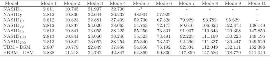
(EBBM,TBM) is established. Table 2 shows the first ten flexural frequencies in non-dimensional form

(ω∗ = ωL_b2q_Eρ) for a simply-supported (SS) beam with a solid square cross-section and a L/b ratio equal to 10. The results are compared with 1D FEM solutions obtained using the commercial code

MSC/NASTRANR_{for which 1D FEM models were constructed by using 2-node CBAR elements.}

The generic one-dimensional MSC/NASTRANR_{model is addressed here as “NAS1D}

el” where the

subscript stands for the number of beam elements. Figure 6 shows the convergence rate of the

MSC/NASTRANR_{models. Based on these results the following remarks can be made:}

• FEM models require much finer meshes to achieve acceptable accuracy, particularly when

higher frequencies are required.

• The DSM being distinct from the FEM, provides exact natural frequencies since it is mesh

independent.

As far as higher-order beam theories are concerned, Tables 3 to 5 show results using both DSM

and FEM solutions based on TE models. Approximate higher-order TE FEM results were obtained

using the recent works by Carrera et al. [40, 41, 43, 42], which showed that TE models are able to

deal with 3D-like solutions. Higher-order TE finite elements with 2 (B2), 3 (B3) and 4 (B4) nodes

were used in the FEM solutions, or in other words, linear, quadratic and cubic approximations along

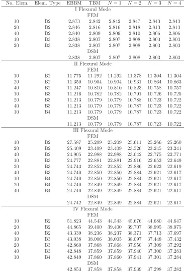
the y-axis were adopted. Table 3 shows the first non-dimensional natural frequency of a SS square

beam with a L/b ratio equal to 100. Column 1 shows the number of finite elements used in the

analysis, whereas the second column quotes the element type. Columns 3 and 4 show the results by

classical beam models (EBBM, TBM) alongside the results in Column 5 where the complete linear

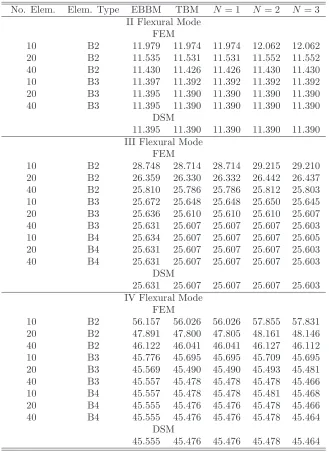
the second-order (N = 2) TE model. For the same structure, Table 4 shows the second, the third

and the fourth natural flexural frequencies for up-to-the-third TE models. Table 5 shows the first

four flexural natural frequencies for a SS square beam withL/b= 10. Classical beam theories, linear

(N = 1), quadratic (N = 2), cubic (N = 3) and fourth-order (N = 4) TE models are considered.

It is clearly shown that, as far as FEM solutions of CUF higher-order models are concerned, the

number of beam elements that are necessary to obtain accurate results provided by the DSM

-increases as natural frequencies as well as beam theory order increase. Figure 7 gives an estimation

of the errors incurred when using FEM as opposed to DSM. The figure shows that FEM gives errors

ranging from 0.005 % (finer mesh) to 19.7 % (coarse mesh).

Figure 8 shows the first three flexural modes of the beam with SS boundary conditions obtained

from the DSM analysis when using a N = 4 TE model. It should be emphasized that DSM results

are mesh independent and the mesh used in Fig. 8 is merely a plotting grid for convenience.

One of the most important features of the DSM is that it provides exact solutions for any kind of

boundary conditions. Moreover, TE higher-order theories are able to take into account several

non-classical effects such as warping, in-plane deformations, shear effects and flexural-torsion couplings.

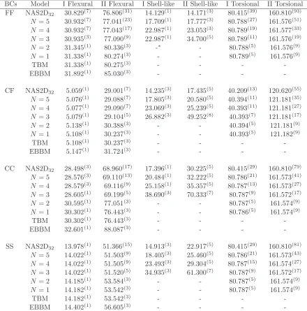
In Table 6, the first two flexural modes and the first two torsional modes for a clamped-free (CF)

short (L/b= 10) square beam are shown. The exact solutions for classical, linear and higher-order

beam theories are also shown and they were computed using the DSM. The results are compared

with 3D FEM models using MSC/NASTRANR_{. The generic three-dimensional FEM solution is}

herein referred to as “NAS3Del” where the subscript “el” stands for the number of elements along

one cross-sectional coordinate. In the results shown in Table 6, 3D FEM models are built using

8-node solid elements with an aspect-ratio equal to 10 were used. Figure 9 shows some representative

modal shapes for the seventh-order TE model of the CF beam. Some comments are relevant:

• According to 3D MSC/NASTRANR_{, the present lower-order DSM-TE models are able to}

characterize the flexural behaviour of solid cross-section beams.

• A fourth-order (N = 4) model is necessary to correctly detect torsional frequencies.

Finally, analyses were carried out for different values of the thickness for a rectangular

cross-section beam with length-to-side ratio, L/a, equal to 10 anda= 0.2. The effect of the aspect ratio,

a/b, on results is shown in Fig. 10, where the variation of the natural frequencies of the first flexural

5.2 Thin-walled Structures

Free vibration analyses of a thin-walled cylindrical beam were carried out next. The cross-section of

the beam is shown in Fig. 11. The outer diameter, d, was set to 2 m, whereas the thickness, t, was

0.02 m. The length-to-diameter ratio, L/d, was taken to be equal to 10. The cylinder was made of

the same material as in the previous examples.

Table 7 shows the natural frequencies of the beam for different BCs, namely, free-free (FF),

clamped-free (CF), clamped-clamped (CC), and simply-supported (SS) BCs. The natural

frequen-cies, in Hz, of the first and second flexural, shell-like and torsional modes are shown. The solutions

for classical beam theories and up-to-fifth-order TE models were obtained using the DSM. The

re-sults are compared to 2D FEM MSC/NASTRANR_{solutions, which are referred to as NAS2D} 32.

The subscript “32” stands for the number of shell elements along the circumference. In the analysis,

4-node shell elements with an aspect-ratio equal to 10 were used. The authors have been highly

selective when presenting the modes. Figure 12 shows the important modes of the cylinder for CC

boundary condition. The following comments arise:

• Only the flexural modes are provided by the classical beam theories.

• Torsional modes are correctly detected by the linear TE (N = 1) model.

• 1D higher-order model are necessary to detect shell-like modes as evident from the 2D FEM

solutions provided by MSC/NASTRANR_.

In Fig. 13 the positions of the first two flexural frequencies in the eigenvalue vector are plotted for

different models of the free-free cylinder. According to Fig. 13, the following remarks can be made:

• In the case of classical theories and the lower-order TE models, the first two flexural frequencies

hold the first two positions of the vector.

• New vibration modes appear as the model is refined. In particular, shell-like modes were found

in between the flexural ones.

The ability of 1D CUF models in dealing with 2D shell-like analyses is widely documented in

previous works, such as [40, 45, 61, 43]. In this paper, the attention is particularly focused on the

advantages related to using the DSM formulation. As it has been said, the DSM provides the exact

solution of the differential equations of the motion once the structural model has been formulated

to confirm the strength and elegance of the DSM when applied to refined 1D CUF models. A

thin-walled beam with the semi-circular cross-section shown in Fig. 14 is analyzed. The geometrical

dimensions are chosen from the literature [62, 63, 64, 57, 65, 66] so that a comparison of the results

is possible. The radius, r, was assumed to be equal to 2.45_×10−2 _{m, the thickness, t, was equal to}

4_×10−3 _{m, the length,L, of the beam was set to 0.82 m. The beam was made of aluminum with the}

Young modulus, E, equal to 68.9 GPa, the Poisson ratio, ν, equal to 0.3, and the density, ρ, equal

to 2700 Kg m−3. Both clamped-free (CF) and simply supported (SS) boundary conditions were

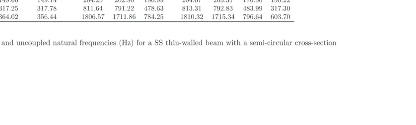
considered. Table 8 shows the first three coupled and uncoupled natural frequencies of the beam for

cantilever boundary conditions and the results from the present theory are compared with those from

the literature. The superiority of the present DSM-CUF models is clearly evident. Table 9 shows

the first three coupled and uncoupled natural frequencies for a SS beam and also shows comparisons

with the literature results. Figure 15 shows both the uncoupled and coupled modal shapes for the

SS semi-circular beam. The following statements are worthy of careful study:

• The present models give good accuracy in the evaluation of the uncoupled frequencies for

thin-walled beams.

• The present DS formulation is preferable to FEM in solving 1D CUF models, especially when

higher-order natural frequencies.

• The increase in the order of the theory provides greater accuracy on the evaluation of the

coupled frequencies. The present sixth-order (N = 6) DSM-TE model is able to compute

the first two coupled frequencies for the SS beam, whereas only the first coupled frequency is

detected if CF boundary conditions are considered.

6

Conclusions

A higher-order exact DS matrix has been developed using the CUF, which allows for the formulation

of any-order beam theories by setting the expansion order as an input of the analysis. The resulting

DS matrix is applied using the Wittrick-Williams algorithm to compute the natural frequencies and

mode shapes of some solid and thin-walled structures. The results agree with those obtained using

MSC/NASTRANR_{FEM models and with those from the literature. The investigation provides}

Acknowledgements

First author acknowledges the Accademia delle Scienze di Torino which made this work possible through the 2012, annual grant named after Ernesto and Ben Omega Petrazzini. The second author

thanks the EPSRC (grant ref: EP/I004904/1) for financial support.

APPENDIX A

Solution of a system of second order differential

equations

A system of differential equations of the second order in xcan be written as

d2y(x)

dx2 = ¨y(x) =f(y(x),y˙(x)) (A.1)

where y(x) = [y1, y2, ..., yn]T are the nunknown functions. This can be written in matrix form as

¨

y(x) =S˜{y1y˙1 y2y˙2 . . . yny˙n}T (A.2)

where ˜S is the matrix of coefficient whose dimension is n_×2n and can be written as:

˜ S=

        

S11 S12 S13 S14 . . . S1(2n−1) S1(2n)

S21 S22 S23 S24 . . . S2(2n−1) S2(2n)

..

. ... ... ... . .. ... ...

Sn1 Sn2 Sn3 Sn4 . . . Sn(2n−1) Sn(2n)

        

(A.3)

With a simple change of variables, the system of second order differential equations can be

trans-formed into a system of first order differential equations. The change of variables is

Z1(x) =y1(x), Z2(x) = ˙y1(x)

Z3(x) =y2(x), Z4(x) = ˙y2(x)

.. .

Z₍₂n−1)(x) =yn(x), Z(2n)(x) = ˙yn(x)

(A.4)

By doing this, a number of first order differential equations, such as ˙Z1 =Z2, ˙Z3 =Z4 and ˙Zn−1 =

Zn, will be added to the system of Eq. (A.1) - and consequently to Eq. (A.2) - which becomes a first

of equations can be re-written in a matrix form as

˙

Z(x) =SZ(x) (A.5)

where the unknown functions are now:

Z=_{Z1 Z2Z3Z4 . . . Z2n−1 Z2n}T ={y1 y˙1y2 y˙2 . . . yny˙n}T (A.6)

and the new matrix of coefficients S, whose dimension now is 2n×2n can be written as:

S=                   

0 1 0 0 . . . 0 0

S11 S12 S13 S14 . . . S1(2n−1) S1(2n)

0 0 0 1 . . . 0 0

S21 S22 S23 S24 . . . S2(2n−1) S2(2n)

..

. ... ... ... . .. ... ...

0 0 0 0 . . . 0 1

Sn1 Sn2 Sn3 Sn4 . . . Sn(2n−1) Sn(2n)

                   (A.7)

The solution of first order differential equations of Eq. (A.5) can be written as

Zi=

2n

X

j=1

Cjδjieλjx (A.8)

where Cj are the constant of integration, λj is the j-th eigenvalue of the matrix S and δji is i-th

value in the j-th eigenvector of the matrix S. For the sake of simplicity, the solution for Z1, i.e. y1

(see Eq. (A.4)) is given in explicit form

y1(x) =C1δ11eλ1x+C2δ21eλ2x+. . .+C2nδ(2n)1eλ2nx (A.9)

if the eigenvectors are written as a matrix δ_{in the following form:}

δ₌         

δ11 δ21 . . . δ(2n)1

δ12 δ22 . . . δ(2n)2

..

. ... . .. ...

δ₁₍₂n) δ2(2n) . . . δ(2n)(2n)

where, forδji,jis the eigenvector number andiis the position in the eigenvector, and the eigenvalues

with the constants are written in the following form:

Ceλx₌n_C

1eλ1xC2eλ2x . . . C2neλ2nx

oT

(A.11)

then the solution of Eq. (A.8) can be written in a more compact matrix form as

Z=δ_Ceλx _(A.12)

APPENDIX B

Forward and backward Gauss elimination

In this section, the procedure to transform the matrixL(Eq. (25)) into˜S(Eq. (A.3)) is described in

details. In matrixL, the coefficients of the second derivatives are located in the columns which are

multiple of 3. In order to decouple the equations, the first row should have -1 in the third column

and zero below it, the second row should have -1 in the sixth column and zeros above and below

that and so on. This matrix has been called Lˆ.

Let us examine a 3 by 9 L matrix which is fully populated. The algorithm can easily be extended

to a matrix ofN by N_×3 dimension. The matrixLˆ and subsequently the matrix˜S(see Eq. (A.3))

can be obtained by following four steps.

L=

     

l11 l12 l13 l14 l15 l16 l17 l18 l19

l21 l22 l23 l24 l25 l26 l27 l28 l29

l31 l32 l33 l34 l35 l36 l37 l38 l39

     

(B.1)

(i) Forward Gauss elimination. Gauss elimination is carried out on entries belowl13,l26. This is

achieved by the following algorithm for the third column

l2i =l2i−

l23

l13

l1i for i= 1, . . . ,9

l3i =l3i−

l33

l13

l1i for i= 1, . . . ,9

(B.2)

and for the sixth column1

l3i =l3i−

l36

l26

l2i for i= 1, . . . ,9 (B.3)

note that the name of the new element has not been changed for sake of simplicity.

The results would be a new L matrix in the following form

L=

     

l11 l12 l13 l14 l15 l16 l17 l18 l19

l21 l22 0 l24 l25 l26 l27 l28 l29

l31 l32 0 l34 l35 0 l37 l38 l39

     

(B.4)

(ii) Backward Gauss Elimination. As before but starting from the third row, ninth column and

eliminating everything that is above that element in order to obtain the following newLmatrix

L=

     

l11 l12 l13 l14 l15 0 l17 l18 0

l21 l22 0 l24 l25 l26 l27 l28 0

l31 l32 0 l34 l35 0 l37 l38 l39

     

(B.5)

(iii) Factorisation. It is required to have -1 on the coefficient corresponding to the second derivative

so to imply that if that coefficient were to be moved on the other side of the differential equation,

its value would be 1. In order to do that the first row is divided by₋l13, the second by−l26and

the third by ₋l39. in this way, the matrix Lˆ can be obtained and it has the following form

ˆ L=

     

l11 l12 −1 l14 l15 0 l17 l18 0

l21 l22 0 l24 l25 −1 l27 l28 0

l31 l32 0 l34 l35 0 l37 l38 −1

     

(B.6)

(iii) Eliminate the columns. By eliminating the columns corresponding to the position 3 and it

multiples, is equal to move the term containing the second derivatives on the other side of the

equations and give the matrix of coefficients associated to the second order differential equation.

This matrix has been called ˜S (see Eq. (A.3)) and following the notation in Eq. (B.6) it can

be written as

˜ S=

     

l11 l12 l14 l15 l17 l18

l21 l22 l24 l25 l27 l28

l31 l32 l34 l35 l37 l38

     

References

[1] L. Euler, De curvis elasticis, Lausanne and Geneva: Bousquet, 1744. (English translation: W.

A. Oldfather, C. A. Elvis, D. M. Brown, Leonhard Euler’s elastic curves, Isis 20 (1933) 72–160).

[2] S. P. Timoshenko, On the corrections for shear of the differential equation for transverse

vibrations of prismatic bars, Philosophical Magazine 41 (1922) 744–746.

[3] S. P. Timoshenko, On the transverse vibrations of bars of uniform cross section, Philosophical

Magazine 43 (1922) 125–131.

[4] V. V. Novozhilov, Theory of elasticity, Pergamon, Elmsford, 1961.

[5] S. P. Timoshenko, J. N. Goodier, Theory of elasticity, McGraw-Hill, 1970.

[6] I. S. Sokolnikoff, Mathematical theory of elasticity, McGraw-Hill, 1956.

[7] N. G. Stephen, Timoshenko’s shear coefficient from a beam subjected to gravity loading, Journal

of Applied Mechanics 47 (1980) 121–127.

[8] J. R. Hutchinson, Shear coefficients for Timoshenko beam theory, Journal of Applied Mechanics

68 (2001) 87–92.

[9] J. J. Jensen, On the shear coefficient in Timoshenko’s beam theory, Journal of Sound and

Vibration 87 (1983) 621–635.

[10] T. Kaneko, On Timoshenko’s correction for shear in vibrating beams, Journal of Physics D:

Applied Physics 8 (1975) 1927–1936.

[11] S. B. Dong, C. Alpdongan, E. Taciroglu, Much ado about shear correction factors in Timoshenko

beam theory, International Journal of Solids and Structures 47 (2010) 1651–1665.

[12] R. El Fatmi, On the structural behavior and the Saint Venant solution in the exact beam theory:

application to laminated composite beams, Computers and Structures 80 (2002) 1441–1456.

[13] R. El Fatmi, Non-uniform warping including the effects of torsion and shear forces. Part I: a

general beam theory, International Journal of Solids and Structures 44 (2007) 5912–5929.

[14] R. El Fatmi, Non-uniform warping including the effects of torsion and shear forces. Part II:

analytical and numerical applications, International Journal of Solids and Structures 44 (2007)

[15] P. Lad´eveze, J. Simmonds, New concepts for linear beam theory with arbitrary geometry and

loading, European Journal Of Mechanics A/Solids 17 (1998) 377–402.

[16] P. Lad´eveze, P. Sanchez, J. Simmonds, Beamlike (Saint-Venant) solutions for fully anisotropic

elastic tubes of arbitrary closed cross-section, International Journal of Solids and Structures 41

(2004) 1925–1944.

[17] O. Rand, Free vibration of thin-walled composite blades, Composite Structures 28 (1994)

169–180.

[18] C. Kim, S. R. White, Thick-walled composite beam theory including 3-D elastic effects and

torsional warping, International Journal of Solids and Structures 34 (1997) 4237–4259.

[19] V. L. Berdichevsky, E. Armanios, A. Badir, Theory of anisotropic thin-walled

closed-cross-section beams, Composites Engineering 2 (1992) 411–432.

[20] V. V. Volovoi, D. H. Hodges, V. L. Berdichevsky, V. G. Sutyrin, Asymptotic theory for static

behavior of elastic anisotropic I-beams, International Journal of Solids and Structures 36 (1999)

1017–1043.

[21] B. Popescu, D. H. Hodges, On asymptotically correct Timoshenko-like anisotropic beam theory,

International Journal of Solids and Structures 37 (2000) 535–558.

[22] W. Yu, V. V. Volovoi, D. H. Hodges, X. Hong, Validation of the variational asymptotic beam

sectional analysis (VABS), AIAA Journal 40 (2002) 2105–2113.

[23] W. Yu, D. H. Hodges, Elasticity solutions versus asymptotic sectional analysis of homogeneous,

isotropic, prismatic beams, Journal of Applied Mechanics 71 (2004) 15–23.

[24] W. Yu, D. H. Hodges, Generalized Timoshenko theory of the variational asymptotic beam

sectional analysis, Journal of the American Helicopter Society 50 (2005) 46–55.

[25] J. S. Kim, K. W. Wang, Vibration analysis of composite beams with end effects via the formal

asymptotic method, Journal of Vibration and Acoustics 132 (2010) 041003.

[26] R. D. Firouz-Abad, H. Haddadpour, A. B. Novinzadehb, An asymptotic solution to transverse

[27] R. Schardt, Eine erweiterung der technischen biegetheorie zur berechnung prismatischer

faltwerke (Extension of the engineer’s theory of bending to the analysis of folded plate

struc-tures), Der Stahlbau 35 (1966) 161–171.

[28] R. Schardt, Generalized beam theory an adequate method for coupled stability problems,

Thin-Walled Structures 19 (1994) 161–180.

[29] N. Silvestre, D. Camotim, First-order generalised beam theory for arbitrary orthotropic

mate-rials, Thin-Walled Structures 40 (2002) 755–789.

[30] N. Silvestre, Second-order generalised beam theory for arbitrary orthotropic materials,

Thin-Walled Structures 40 (2002) 791–820.

[31] N. Silvestre, Generalised beam theory to analyse the buckling behaviour of circular cylindrical

shells and tubes, Thin-Walled Structures 45 (2007) 185–198.

[32] R. Bebiano, N. Silvestre, D. Camotim, Local and global vibration of thin-walled members

subjected to compression and non-uniform bending, Journal of Sound and Vibration 345 (2008)

509–535.

[33] K. Washizu, Variational Methods in Elasticity and Plasticity, Pergamon, Oxford, 1968.

[34] K. Kapania, S. Raciti, Recent advances in analysis of laminated beams and plates, part I: Shear

effects and buckling, AIAA Journal 27 (1989) 923–935.

[35] K. Kapania, S. Raciti, Recent advances in analysis of laminated beams and plates, part II:

Vibrations and wave propagation, AIAA Journal 27 (1989) 935–946.

[36] E. Carrera, A class of two dimensional theories for multilayered plates analysis, Atti Accademia

delle Scienze di Torino, Memorie Scienze Fisiche 19-20 (1995) 49–87.

[37] E. Carrera, Theories and finite elements for multilayered, anisotropic, composite plates and

shells, Archives of Computational Methods in Engineering 9 (2002) 87–140.

[38] E. Carrera, Theories and finite elements for multilayered plates and shells: a unified compact

formulation with numerical assessment and benchmarking, Archives of Computational Methods

in Engineering 10 (2003) 216–296.

[39] E. Carrera, S. Brischetto, Analysis of thickness locking in classical, refined and mixed

[40] E. Carrera, G. Giunta, M. Petrolo, Beam Structures: Classical and Advanced Theories, John

Wiley & Sons, 2011. DOI: 10.1002/9781119978565.

[41] E. Carrera, G. Giunta, P. Nali, M. Petrolo, Refined beam elements with

arbi-trary cross-section geometries, Computers and Structures 88 (2010) 283–293. DOI:

10.1016/j.compstruc.2009.11.002.

[42] E. Carrera, M. Petrolo, E. Zappino, Performance of CUF approach to analyze the

struc-tural behavior of slender bodies, Journal of Strucstruc-tural Engineering 138 (2012) 285–297. DOI:

10.1061/(ASCE)ST.1943-541X.0000402.

[43] E. Carrera, M. Petrolo, P. Nali, Unified formulation applied to free vibrations finite element

analysis of beams with arbitrary section, Shock and Vibrations 18 (2011) 485–502. DOI:

10.3233/SAV-2010-0528.

[44] E. Carrera, M. Petrolo, A. Varello, Advanced beam formulations for free vibration analysis

of conventional and joined wings, Journal of Aerospace Engineering 25 (2012) 282–293. DOI:

10.1061/(ASCE)AS.1943-5525.0000130.

[45] M. Petrolo, E. Zappino, E. Carrera, Refined free vibration analysis of one-dimensional structures

with compact and bridge-like cross-sections, Thin-Walled Structures 56 (2012) 49–61. DOI:

10.1016/j.tws.2012.03.011.

[46] J. R. Banerjee, Dynamic stiffness formulation for structural elements: a general approach,

Computers and Structures 63 (1997) 101–103.

[47] J. R. Banerjee, Coupled bending-torsional dynamic stiffness matrix for beam elements,

Inter-national Journal of Numerical Methods in Engineering 28 (1989) 1283–1298.

[48] J. R. Banerjee, Free vibration analysis of a twisted beam using the dynamic stiffness method,

International Journal of Solids and Structures 38 (2001) 6703–6722.

[49] J. R. Banerjee, Free vibration of sandwich beams using the dynamic stiffness method,

Com-puters and Structures 81 (2003) 1915–1922.

[50] J. R. Banerjee, Development of an exact dynamic stiffness matrix for free vibration analysis of

[51] J. R. Banerjee, C. W. Cheung, R. Morishima, M. Perera, J. Njuguna, Free vibration of a

three-layered sandwich beam using the dynamic stiffness method and experiment, International

Journal of Solids and Structures 44 (2007) 7543–7563.

[52] F. W. Williams, W. H. Wittrick, An automatic computational procedure for calculating natural

frequencies of skeletal structures, International Journal of Mechanical Sciences 12 (1970) 781–

791.

[53] W. H. Wittrick, A unified approach to initial buckling of stiffened panels in compression,

International Journal of Numerical Methods in Engineering 11 (1968) 1067–1081.

[54] W. H. Wittrick, F. W. Williams, Buckling and vibration of anisotropic or isotropic plate

assemblies under combined loadings, International Journal of Mechanical Sciences 16 (1974)

209–239.

[55] M. Boscolo, J. Banerjee, Dynamic stiffness formulation for composite Mindlin plates for exact

modal analysis of structures. Part I: Theory, Computers & Structures 96-97 (2012) 61–73. DOI:

10.1016/j.compstruc.2012.01.002.

[56] M. Boscolo, J. Banerjee, Dynamic stiffness formulation for composite Mindlin plates for exact

modal analysis of structures. Part II: Results and applications, Computers & Structures 96-97

(2012) 74–83. DOI: 10.1016/j.compstruc.2012.01.003.

[57] W. H. Wittrick, F. W. Williams, A general algorithm for computing natural frequencies of

elastic structures, Quarterly Journal of Mechanics and Applied Mathematics 24 (1971) 263–

284.

[58] S. W. Tsai, Composites Design, 4th ed., Dayton, Think Composites, 1988.

[59] J. N. Reddy, Mechanics of laminated composite plates and shells. Theory and Analysis, 2nd

ed., CRC Press, 2004.

[60] W. H. Wittrick, F. W. Williams, A general algorithm for computing natural frequencies of

elastic structures, Quarterly Journal of mechanics and applied sciences 24 (1970) 263–284.

[61] E. Carrera, A. Pagani, M. Petrolo, Component-wise method applied to vibration of wing