A compilation of the full PDDL+ language into SMT

A Compilation of the Full PDDL+ Language into SMT

Michael Cashmore, Maria Fox, Derek Long, Daniele Magazzeni

firstname.lastname@kcl.ac.uk

Abstract

Planning in hybrid systems is important for dealing with real-world applications. PDDL+ supports this representation of domains with mixed discrete and continuous dynamics, and supportseventsandprocessesmodeling exogenous change. Motivated by numerous SAT-based planning approaches, we propose an approach to PDDL+ planning through SMT, de-scribing an SMT encoding that captures all the features of the PDDL+ problem as published by Fox and Long (2006). The encoding can be applied on domains with nonlinear contin-uous change. We apply this encoding in a simple planning algorithm, demonstrating excellent results on a set of bench-mark problems.

1

Introduction

PDDL+ planning is a growing area in the planning com-munity, mainly motivated by the need to deal with real-world applications. PDDL+ (Fox and Long 2006) is the extension of PDDL designed to model hybrid dynamics, which are featured by a number of applications of inter-est for planning, and PDDL+ is pushing forward the use of planning in real-world domains (e.g., (Campion et al. 2013; Fox, Long, and Magazzeni 2011)). A number of approaches have been proposed that can handlesubsetsof PDDL+. No-toriously, most planners cannot handle events, or are limited to linear process models, as described later.

In this paper we propose a new approach for PDDL+ plan-ning that can handle the whole set of PDDL+ features and respects Fox and Long’s semantics. Our work builds on pre-vious SAT encodings of planning problems (Kautz and Sel-man 1996; Rintanen 2010). We propose an SMT encoding of PDDL+ domains.

Planning through SMT is not new, although the approach presented here makes important contributions to PDDL+ planning through SMT. A recent approach, dReach, de-scribed in (Bryce et al. 2015) uses a non-linear SMT solver for planning in hybrid systems. That approach is promis-ing, although it suffers some important limitations. Firstly, it does not use PDDL+, as it relies on the language of dReach, in which the hybrid problems have to be manually encoded. Secondly, dReach can only handle a restricted subset of the language features contained in PDDL+, and, in particular, they cannot handle events, which are a significant feature of

PDDL+. Thirdly, dReach is tailored to be used only with the dReal solver (Gao, Avigad, and Clarke 2012).

In this paper, we propose a new encoding for PDDL+ which overcomes these limitations, and gives much bet-ter results in all the tested domains. In particular, our en-coding is able to capture all features of PDDL+ (including events) and works by directly translating standard PDDL+ domain and problem files. Furthermore, we are careful to correctly capture themustsemantics of PDDL+ (which con-strains how processes and events interact with each other and with actions). Also, we model the precise semantics of ε -separation of effects and action preconditions (Fox and Long 2006). The output of the translation is a standard SMT en-coding that can be used with any SMT solver in the theory of quantifier-free nonlinear arithmetic (QF NRA). Further-more, our approach proves to also be efficient in proving plan-non-existence, along with dramatically improving over dReach in solvable problems.

In terms of the dynamics our approach can handle, we can deal with nonlinear polynomial change. Moreover, when an instantaneous event triggers another, this can cause a cas-cade of events which all trigger simultaneously. Following the PDDL+ semantics (Fox and Long 2006), we assume to have a bound on the length of a causal chain of instantaneous events.

In the following we first introduce hybrid domains and PDDL+. We then present the new encoding, and use a work-ing example to show how PDDL+ features are encoded in SMT. The overall approach is evaluated on a set of bench-mark problems, and compared with previous works.

2

Hybrid Systems and PDDL+

A hybrid system is one in which there are both continu-ous control parameters and discrete logical modes of op-eration. It represents a powerful model to describe the dy-namic behaviour of modern engineering artefacts. Hybrid systems frequently occur in practice, e.g., in robotics or em-bedded systems. Dealing with hybrid systems is becoming more and more an important challenge, as many real-world scenarios feature a mixture of discrete and continuous be-haviours. Some example applications include coordination of activities of a planetary lander, oil refinery management, autonomous vehicles, chemical plant (Della Penna et al.

2010), smart grid (Campion et al. 2013), and battery man-agement (Fox, Long, and Magazzeni 2011). Such scenarios motivate the need to reason with mixed discrete-continuous domains.

The theory of hybrid automata, introduced by Henzinger (Henzinger 1996), represents a well-defined formalism for describing hybrid systems.

2.1

Hybrid Automata

Intuitively, hybrid automata (Henzinger 1996) are finite state automata extended with continuous variables that evolve over time. More formally, we have the following:

Definition 1 (Hybrid Automaton). Ahybrid automatonis a tupleH= (Loc,Var,Init,Flow,Trans,I), where

• Loc is a finite set of locations,Var = {x1, . . . , xn} is a set of real-valued variables,Init(`)⊆Rn is the set of initial values forx1, . . . , xnfor all locations`.

• For each location `,Flow(`)is a relation over the vari-ables inVarand their derivatives of the form

˙

x(t) =Ax(t) +u(t), u(t)∈ U,

wherex(t) ∈ _Rn_{,A is a real-valuedn×nmatrix and}

U ⊆Rnis a closed and bounded convex set.

• Transis a set of discrete transitions. A discrete transition

t∈Trans is defined as a tuple(`, g, ξ, `0_)where`and`0

are the source and the target locations, respectively,g is the guard oft(given as a linear constraint), andξis the update oft(given by an affine mapping).

• I(`)⊆<sub>R</sub>n<sub>is an invariant for all locations`.</sub>

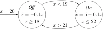
An example is the hybrid automaton for a thermostat de-picted in Figure 1. Here, the temperature is represented by the continuous variable x. In the discrete location corre-sponding to the heater being off, the temperature falls ac-cording to the flow conditionx˙ =−0.1x, while, when the heater is on, the temperature increases according to the flow conditionx˙ = 5−0.1x. The discrete transitions state that the heater maybe switched on when the temperature falls below 19 degrees, and switched off when the temperature is greater than 21 degrees. Finally, the invariants state that the heater can be on (off)onlyif the temperature is not greater than 22 degrees (not less than 18 degrees).

Off

˙

x=−0.1x x≥18

On

˙

x= 5−0.1x x≤22

x >21

x <19

x= 20

Figure 1: Thermostat hybrid automaton

2.2

PDDL+ Planning

PDDL+ is the extension of PDDL that allows modelling of mixed discrete-continuous domains, through continuous processes and events. PDDL+ is based on hybrid automata semantics, although there are some key difference, such as

the must semantics. Continuous processes are triggered as soon as their precondition becomes true, and in this sense theymustbe triggered. Exogenous events follow the same semantics. The rationale behind this is that processes and events are used to model changes that are initiated by chang-ing in the world, therefore they are not under the control of the executive and are triggered immediately (see (Bogo-molov et al. 2014)) for more details).

Various techniques and tools have been proposed to deal with hybrid domains (Penberthy and Weld 1994; McDer-mott 2003; Li and Williams 2008; Coles et al. 2012; Shin and Davis 2005). More recent approaches in this direction have been proposed by (Bogomolov et al. 2014), where the close relationship between hybrid planning domains and brid automata is explored, and (Bryce et al. 2015) where hy-brid domains are handled using SMT.

Nevertheless, none of these approaches are able to handle the full set of PDDL+ features, namely nonlinear domains with processes and events.

On the other hand, many works have been proposed in the model checking and control communities to han-dle hybrid systems. Some examples include (Cimatti et al. 2015; Cavada et al. 2014; Cimatti, Mover, and Tonetta 2012; Tabuada, Pappas, and Lima 2002; Maly et al. 2013), sampling-based planners (Karaman et al. 2011; Lahijanian, Kavraki, and Vardi 2014). Another related direction is falsi-ficationof hybrid systems (i.e., guiding the search towards the error states, that can be easily cast as a planning problem) (Plaku, Kavraki, and Vardi 2013). However, while all these works aim to address a similar problem, that cannot be used to handle PDDL+ models. Some recent works (Bogomolov et al. 2014; 2015) are trying to define a formal translation be-tween PDDL+ and standard hybrid automata, but so far only an over-approximation has been defined, that allows the use of those tools only for proving plan non-existence.

To date, the only viable approach in this direction is PDDL+ planning via discretisation. UPMurphi (Della Penna, Magazzeni, and Mercorio 2012), which implements the discretise and validate approach, is able to deal with the full range of PDDL+ features.

3

PDDL+ as SMT

PDDL+ supports the representation of domains with mixed discrete-continuous dynamics, providing a flexible model of continuous change. In this section we will describe the PDDL+ planning model, as an extention of PDDL2.1. Then, we will describe our encoding of a PDDL+ planning prob-lem as an SMT formula.

Definition 2 (PDDL2.1 Planning Problem). A PDDL2.1 planning problem is a tuple Π := {P, V, A, I, G}, where

P is a set of propositions; V is a vector of real variables, called fluents; both are manipulated byA, a set of durative and instantaneous actions.I(P, V)is a fuction overP∪V

which describes the initial state of the problem. Similarly

G(P, V)is a function that describes thegoal condition. A durative actionais described as a tuple:

whereprea represents the action’s preconditions – condi-tions that must hold for the action to be applied –ef fa rep-resents the action’s effects, anddurais a duration constraint,

a conjunction of numeric constraints corresponding to the duration of the actiona.

A single condition is either a single propositionp∈P, or a numeric constraint overV. A precondition is a conjunction of zero or more conditions. Each durative actionAhas three disjoint subsets of preconditions:

pre`a, pre↔a, preaa⊆prea

These represent the conditions that must hold at its start, throughout its execution, and at the end of the action, re-spectively.

Action effects are described by seven subsets: eff+_{`a</sub>,eff−<sub>`a},effnum_`a , eff+_aa,eff−_aa,effnum_aa , eff_↔a

eff_↔ais a conjunction ofcontinuousnumeric effectseff_↔, which are applied continuously while the action is execut-ing. The rest are instantaneous effects, adding or removing propositions, or numeric effects. These are bound to the start or end of the action. For example,eff+_`adenotes the propo-sitions added at the start of the action. Semantically, the val-ues of such instantaneous effects can be exploited to support actions only after a small of timeε(Fox and Long 2003).

As a special case,instantaneousactions have duration0, have only one set of preconditions prea; and three sets of effectseff+_a,eff−_a, andeffnum_a .

PDDL+ extends PDDL2.1 to support the modelling of ex-ogenous events, reflecting changes that are initiated by the environment. PDDL+ introduces the new constructs of pro-cessesandevents.

As an analogue, events are akin to instantaneous actions: if an event’s preconditionspreaare satisfied, it occurs, yield-ing the event’s instantaneous effects. Similarly, processes are akin to durative actions. The critical distinctions between processes and events, and actions, is that a process/event will automatically occur as soon as its precondition is satisfied; whereas an action will only happen if chosen to be executed in the plan. Furthermore, that the values of events become available instantaneously. Therefore, if one evente1is trig-gered, with effects that satisfy another evente2and trigger a processp1, thene1,e2, and the start ofp1all happen at the same time-point. It is due to this behaviour that we place a bound on the number of cascading (parallel) events. Definition 3 (PDDL+ Planning Problem). A PDDL+ planning problem is a tupleΠ+ :=

P, V, A, P s, E, I, G , in whichP is a set of propositions; V is a vector of real variables, called fluents; andAis a set of durative and in-stantaneous actions.P sis a set of processes, andEa set of events.I(P, V)andG(P, V)represent the initial state and goal condition respectively.

3.1

Encoding of PDDL+ Domains

In this section we describe how we encode a PDDL+ do-main. First, we introduce the notion ofhappening, that is

used to capture the change in the state at a given time point, due to the effects of actions, processes or events happen-ing at that time point. Namely, each happenhappen-ing encodes the causal chain of processes, events and instantaneous actions which might occur simultaneously at a given time point. Note that, according to the PDDL+ semantics, effects of ac-tions applyεtime after they occur, therefore we need to con-sider the change happening in the time intervalst+ε.

An example of happening is shown in Figure 2.

t t+ε

P0∪V0∪E0∪P s0

P1∪V1∪E1∪P s1

PB∪VB∪EB∪P sB∪A P+∪V+

Figure 2: A single happening, with a bound ofBcascading events. The happening occurs at timet, at which there are several sets of state variables. These sets describe a causal chain of instantaneous events and processes triggers. Ac-tions are included at the end of this chain.

Formally, we have the following

Definition 4 (Happening). A happening is the tuple x:=

{t,P ,ˆ V ,ˆ P s,ˆ E,ˆ A, Pˆ +_{, V}+_{}, where:}

• tis the current time point;

• Pˆ = {P0, . . . , PB} represents the causal change in the propositional state variablesP at timet;

• Vˆ = {V0, . . . , VB} represents the causal change in the

real state variablesV at timet;

• P sˆ ={P s0, . . . , P sB}represents the chain of active pro-cessesP sat timet;

• Eˆ = {E0, . . . , EB} represents the chain of events

trig-gered at time timet;

• Aˆis the set of actions applied at timet.

• P+ _{is the value of propositional state variables at time} t+ε;

• V+_{is the value of real state variables at timet+ε.} For our encoding we split durative actions as two intan-taneous actions, representing the start and end of the action, and one process representing the continuous numerical ef-fects and invariant.

and the continuous change is not limited to first order deriva-tives.

Having defined happenings, a PDDL+ model can be de-scribed as a bounded set of happeningsX:={x1...xn} en-coded as an SMT formula, such that any proof for the SMT formula represents the trace of a valid plan forΠ+. Theplan

corresponding to that trace is the set of action assignments ( ˆA)1∪...∪( ˆA)n.

We first describe the encoding of a single happening, and then describe the encoding of the formula forΠ+.

Encoding of a Happening Following from Definition 4, we encode a happeningxas follows:

x:=

* _{t, P}

0, ..., PB, V0, ..., VB, E0, ..., EB, P s0, ..., P sB, A, P+_{, V}+_{, f low}

V, durP s

+

We recall that we assume a boundBon the length of the causal chain of events at each time point. If the causal chain is longer than this, then a valid plan will not be found.

Any actions applied at time pointtare represented in the setA. The setsP+andV+describe the values of the state variables at time(t+ε), containing the instantaneous effects of these actions, according to the PDDL+ semantics (Fox and Long 2006). Actions can only be applied together in the same happening if they are not mutually exclusive (mutex). Actionsa1anda2can be applied simultaneously if:

prea1∩(eff+a2∪eff

−

a2∪eff num a2 ) =∅ prea2∩(eff+a1∪eff

−

a1∪eff num a1 ) =∅ eff+a1∩eff−a2=eff

+

a2∩eff−a1=∅

{v1|∀v1∈effnum_a1 } ∩ {v2|∀v2∈effnum_a2 }=∅

The setf lowV := {f lowv|∀v ∈ V}is a numerical

ex-pression that represents the change in value ofv from this time point to the next. Finally,durP s:={durps|∀ps∈P s}

represents the remaining duration of each process.durpsis

constrained to be positive if and only if the process is cur-rently executing.

The constraints within a happening are shown in Figure 3.

Proposition and real variable supportconstraints ensure that the value of propositions (H1-H2) and real variables (H3) re-mains consistent fromP0∪V0toPB∪VB.Event precondi-tions and effectsconstraints enforce that an event is triggered if and only if its precondition holds (H4) and that if an event is triggered, its effects are present in the next set (H5).

Action preconditions and effects ensure the same rules apply for actions in A; their preconditions must hold in

PB∪VB (H6) and their effects are enforced inP+ _∪V+ (H7). Support across epsilon separation ensures that the value of propositions (H8-H9) and real variables (H10) re-mains consistent fromPB∪VBtoP+∪V+.

Process triggeringconstraints enforce that a process is ac-tive if and only if its preconditions are satisfied in each set

P0∪V0 toPB ∪VB (H11). It also enforces that the real

variabledurps for each process is greater than or equal to zero (H12), and that if and only if the process is active at the end of the causal chain of events, then the duration is strictly

greater than zero (H13). These constraints will be used to ensure that a process cannot finish outside of a happening.

Finally,Action mutexesare included as a collection of bi-nary constraints, enforcing that no two mutex actions can be applied simultaneously. For each pair of mutex actions, denoteda∦a0, one must be false (H14).

Encoding of a Planning Problem Π+ The existence of a plan for aPDDL+ planning problemΠ+with boundnis proved by building the SMT formulaΠ+nin the theory of

quantifier-free (nonlinear) real arithmetic with ncopies of the set of variablesx(x1...xn) forn≥1. Aplan forΠ+is

the assignment to the action variables in any proof ofΠ+n.

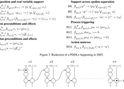
The encoding is illustrated by Figure 4.

The constraints for a happening in Figure 3 are copied for each happeningx0...xn. Additional constraints in the SMT formulaΠ+nare shown in Figure 5 and explained below.

The Instance description constraints enforce the initial state to hold in the first happening (P1), and that the goal is achieved in the final happening (P2). Also, they constrain the timing of happenings to enforce epsilon separation (P3-P4).

Proposition support simply ensures that the discrete state variablesPdo not change between two happenings (P5-P6).

Invariantconstraints ensure that the continuous numeric change between happenings is valid. This is achieved in three parts. First (P7) ensures that if a process is active in the previous happening, its duration is decreased by the time between happenings. This constraint, in combination with constraints (P12-P13) of figure 3, ensure that a process can-not end between happenings. Note that a process can remain active over intervals spanning multiple happenings.

Constraint (P8) enforces the invariant of the process. If a process is active, then the precondition of the process is active over the whole interval between happenings, and if the process is not active, then the precondition is false over the whole interval. For constraints over real valued variables, this is done by checking the value either side of the interval. For nonlinear change, it is necessary to include the following additional constraint:

psi→

A

^

a=1

(d

a_f

dta)i( da_f

dta)i+1>= 0

wheref is the numeric, non-constant part of the invariant, and where the(A+ 1)th derivative off is identically zero. This ensures that the derivatives of the function do not cross zero over the interval, thus a fluctuating value off cannot violate the invariant condition betweeniandi+ 1.

Constraint (P9) similarly ensures that an event is not trig-gered during an interval. Here ¬(pre↔e) is the condition

thatpreedoes not hold over the whole interval.

Continuous change on real variablesis enforced by cal-culating the change over the interval (P10) and applying it to each real variable (P11). In order to calculate the change, the indefinite integral of the process’ effects upon the vari-able must be computed. This is done automatically using the computer algebra system (CAS) SymPy (SymPy 2013).

Proposition and real variable support

H1. VB−1

i=0 V

p∈Ppi+1→(pi

W

e|p∈ef fe+ei) H2. VB−1

i=0 V

p∈P¬pi+1→(¬piWe|p∈eff−

e ei) H3. VB−1

i=0 V

v∈V(

V

e|v∈effnum

e ¬vi)→(vi+1=vi) Event preconditions and effects

H4. VB

i=0 V

e∈Eei↔(pree)i

H5. VB−1

i=0 V

e∈Eei→(effe)i+1 Action preconditions and effects

H6. V

a∈Aa→(prea)B

H7. V

a∈Aa→(effa)+

Support across epsilon separation

H8. V

p∈Pp +_→(p

BWa|p∈eff+

a a) H9. V

p∈P¬p

+_→(¬p

BWa|p∈eff−

a a) H10. V

v∈V(

V

a|v∈effnum

a ¬a)→(v

+_=vB)

Process triggering

H11. VB

i=0 V

ps∈P spsi↔(preps)i

H12. V

ps∈P sdurps>= 0

H13. V

ps∈P spsB↔(durps>0)

Action mutexes

H14. V

a∈A

V

a0_∈A|a∦a0(¬a∨ ¬a0)

Figure 3: Reduction of a PDDL+ happening to SMT.

I

G

x

1

t1 (t1 +ε)

x

2

t2 (t2 +ε)

x

3

t3 (t3 +ε)

xn

tn(tn+ε)

Figure 4: A plan is found by building a formula with ncopies of the set of variablesx: x1...xn. Each Happening models

discrete change. Between happenings there is only continuous numerical change. The initial state is modelled inx1, and the goal constraints are added toxn.

Instance description

P1. I((P0)1∪(V0)1) P2. G((P+)n∪(V+)n)

P3. t1= 0 P4. Vn

i=2ti ≥ti−1+ε Proposition support

P5. Vn

i=2 V

p∈P(p0)i →(p+)i−1 P6. Vn

i=2 V

p∈P¬(p0)i→ ¬(p+)i−1

Invariants

P7. Vn

i=2 V

ps∈P s(psB)i−1→((durps)i = (durps)i−1+ti−ti+1) P8. Vn−1

i=1 V

ps∈P s(psB)i↔(pre↔ps)i

P9. Vn−1

i=1 V

e∈E¬(pre↔e)i

Continuous change on real variables

P10. Vn−1

i=1 V

v∈V(f lowv)i =

Rti+1

ti ∪ps∈P s(eff

num

↔ps[v])idt

P11. Vn

i=2 V

v∈V((v0)i= (v+)i−1+ (f lowv)i−1)

Figure 5: Reduction of PDDL+ planning problemΠ+to SMT.

outside the solver, during the encoding. Hence the integra-tion is done only once for each domain.

4

Example: Simple Generator

We will walk through the encoding of a simple PDDL+ problem, the simple generator problem. The domain is shown in Figure 6. The initial state asserts that there is one generator; the generator’s capacity C; and initial fuel level F. The goal state is that the generator has been run:

(generator-ran).

We will show the encoding of three happeningsx1andx2 – the minimum number of steps required to solve this prob-lem. As there are no events in the domain, we will impose a

boundB = 0on the number of cascading events. Therefore each happening is the set:

xi:= *

gen ran0, ref ueling0 :Bool f uelLevel0, capacity0 :Real gen ran+, ref ueling+ :Bool f uelLevel+, capacity+ :Real gen start, gen end, gen process :Bool

dur gen process :Real

f low f uelLevel, f low capacity :Real

+

(define (domain simple_generator) (:requirements

:fluents :durative-actions :duration-inequalities :adl :typing)

(:types generator) (:predicates

(generator-ran)

(refueling ?g - generator)

(:functions

(fuelLevel ?g - generator) (capacity ?g - generator))

(:durative-action generate :parameters (?g - generator) :duration (= ?duration 1000)

:condition (over all (>= (fuelLevel ?g) 0)) :effect (and

(decrease (fuelLevel ?g) (* #t 1)) (at end (generator-ran)))))

Figure 6: Simplified PDDL+ generator domain

x1 x2

t1:= 0 t2:= 1000

f uelLevel0= 1020.0

f uelLevel+_{= 1020.0}

capacity0= 1060.0

capacity+= 1060.0

f uelLevel0= 20.0

f uelLevel+_{= 20.0}

capacity0= 1060.0

capacity+= 1060.0

gen start gen process ref ueling+

ref ueling0

gen end gen ran+

dur gen process= 1000.0

f low f uelLevel=−1000.0

f low capacity= 0

dur gen process= 0.0

f low f uelLevel= 0.0

f low capacity= 0

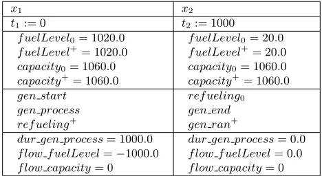
Table 1: A plan for the simple generator domain, as assign-ment to the variables. Boolean variables are shown in the table if and only if they are assigned true.

The formula forΠ+consists of the following constraints in conjunctive normal form (CNF): the instance description enforces the initial state, the goal condition, and that that the second happening is at leastεlater than the first.

(0 =t1)

¬(gen ran0)1

¬(ref ueling0)1 (F = (f uelLevel0)1) (C= (capacity0)1) (gen ran+)2 (t2>= (t1+ε))

Proposition support constraints (between happenings) en-sure that discrete state stays constant during the interval1:

(gen ran+)1= (gen ran0)2 (ref ueling+₎

1= (ref ueling0)2

1

All the formulae in the following are represented in conjunc-tive normal form (CNF).

Invariant constraints ensure that the durative action’s over-all condition holds over an interval in which its associated process is active, and that the durative action’s duration is properly updated across the interval:

(gen process)1→((f uelLevel+)1>= 0) (gen process)1→((f uelLevel0)2>= 0) (gen process)1→

((dur gen process)2=

((dur gen process)1+t1−t2))

The continuous change over real variables is defined and en-forced by thef lowvariables:

(gen process)1→(f low f uelLevel)1= Rt2

t1(−1.0)dt

¬(gen process)1→(f low f uelLevel)1= 0 (f low capacity)1= 0

(f uelLevel0)2= (f uelLevel+)1+ (f low f uelLevel)1 (capacity0)2= (capacity+)1+ (f low capacity)1

Proposition support constraints (within happenings) and ac-tion precondiac-tions and effects, describe the discrete changes that occurs within a happening, fori={1,2}:

(gen ran+₎

i→(gen ran0)i∨(gen end)i

¬(gen ran+₎

i→ ¬(gen ran0)i

(ref ueling0)i= (ref ueling+)i

(f uelLevel0)i= (f uelLevel+)i

(capacity0)i= (capacity+)i

(gen start)i→(gen process)i

(gen end)i→(gen ran+)i

(gen end)1↔(gen process)1∧ ¬(gen process)2

Process triggering constraints work together to ensure that the duration of the durative action is within the constraints of the durative action, and that it begins and ends within the happenings:

(dur gen process)1>= 0

¬(gen process)1↔((dur gen process)1= 0) (gen start)1←((dur gen process)1= 1000.0)

¬(gen start)1←((dur gen process)1= 0.0)

Finally, action mutexes are included. In our encoding, we make the starts and ends of durative actions mutually exclu-sive, eg. fori={1,2}:

¬(gen start)i∨ ¬(gen end)i

5

Results

Domain Tool 1 2 3 4 5 6 7 8

Generator lin-ear

SMTPlan+ 0.02 0.03 0.02 0.01 0.02 0.02 0.02 0.02

dReach 2.87 - - -

-UPMurphi 0.2 18.2 402.34 - - - -

-Generator nonlinear

SMTPlan+ 0.02 0.02 0.02 0.02 0.02 0.02 0.02 0.02

dReach 5.16 - - -

-UPMurphi - - -

-Generator nonlin. events

SMTPlan+ 0.04 0.04 0.04 0.04 0.04 0.04 0.05 0.05

dReach x x x x x x x x

UPMurphi 658.18 - - -

-Generator Tor-ricelli

SMTPlan+ 0.03 0.03 0.15 0.92 0.04 0.05 0.09 0.50

dReach x x x x x x x x

UPMurphi - - -

-Car

SMTPlan+ 0.02 0.02 0.02 0.02 0.02 0.02 0.01 0.02 dReach 1.30 1.41 1.48 1.53 1.47 1.54 1.40 1.53

UPMurphi 28.44 386.5 - - -

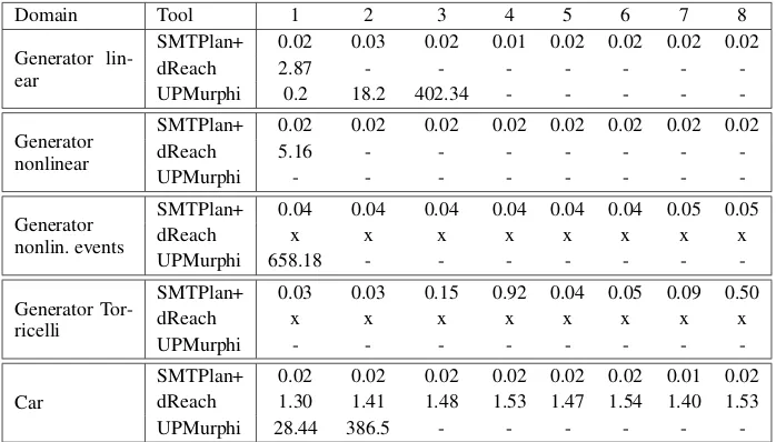
-Table 2: Results in seconds for solvable instances. Instance numbers correspond to number of tanks (generator) and number of acceleration steps (car). Abbrev.: -: tool still running after 30 minutes, ’.’: tool ran out or memory, x: tool cannot handle the problem.

nSMT instances being solved. The SMT solver we use is z3 (De Moura and Bjørner 2008).

We compare our approach (called SMTPlan+) against existing PDDL+ planner UPMurphi (Della Penna, Mag-azzeni, and Mercorio 2012), and with dReach (Bryce et al. 2015), using the SMT solver dReal (Gao, Avigad, and Clarke 2012), on domains without events. We use the gen-erator andcar domains (Bogomolov et al. 2014). The ex-periments were run using 8GB of RAM and a 30 minute timeout. All test domains, problems and plans are available at:[Website omitted for author anonymity].

Generator The generator domain is a PDDL+ benchmark problem that revolves around refueling a diesel-powered generator which has to run for a given duration without over-flowing or running dry. To test scalability, the number of tanks is increased while decreasing the initial generator fuel level.

We consider four versions of this domain: linear, simplified-nonlinear (the same used in (Bryce et al. 2015)), nonlinear with events, and the Torricelli nonlinear (Howey and Long 2003). Note that the latter version uses the Torri-celli’s Law (which is too complex for dReach), and hence the fuel level in a refueling tank (Vf uel) is calculated by:

Vf uel= (−ktr+

p

Vinit)2 tr∈

0,

√

Vinit k

(1)

whereVinit is the initial volume of fuel in the tank,kis the fuel flow constant (which depends on gravity, size of the drain hole, and the cross-section of the tank), andtr is the

time of refueling (bounded by the fuel level and the flow constant).

Here is an example of plan found by SMTPlan+ for the Torricelli nonlinear generator (Fuel level 960, Generator ca-pacity 990):

0.0: generate [1000.0] 959.0: refuel_tank1 [10.0] 959.0: refuel_tank2 [10.0]

Car The car domain is another PDDL+ benchmark (Fox and Long 2006) where a vehicle has to cover a given dis-tance and have a zero velocity at the end, and the ac-tions available are accelerate and decelerate that incre-ments or decreincre-ments by 1 the current velocity, respec-tively. To test scalability, the bound on maximum acceler-ation/deceleration is increased.

Our results for solvable instances are reported in table 2. On both linear and nonlinear domains, SMTPlan+ outper-forms all other planners in time to solve and in number of in-stances solved. In all domains, SMTPlan+ scales very well. For these domains, the number of happenings required is small, thus the minimal SMT encoding required to solve the problem is also small. The iterative deepening algorithm is able to reach a satisfiable encoding, and produce a plan very quickly.

dReach also performs iterative deepening, but performs more poorly. This is due to the semantics of dReach; in the dReach domain and problem description, each mode of con-tinuous change must be explicitly defined, and the number of modes increases exponentially with the number of pro-cesses and durative actions (eg. the files for 1, 2, 3 and 4 tanks problems are respectively 91, 328, 1350, 5762 lines long). Furthermore, the bound is not on the number of hap-penings, but on the number of mode changes, which does not allow for parallel execution of actions.

Domain Tool 1 2 3 4 5 6 7 8

Generator lin-ear

SMTPlan+ 0.01 0.02 0.16 2.84 390.86 - -

-dReach 2.57 189.94 - - -

-UPMurphi 0.90 29.42 - - -

-Generator nonlinear

SMTPlan+ 0.01 1.95 33.48 - - - -

-dReach 2.43 212.43 - - -

-UPMurphi - - -

-Generator nonlin. events

SMTPlan+ 0.02 18.58 21.83 - - - -

-dReach x x x x x x x x

UPMurphi 658.18 - - -

-Generator Toricelli

SMTPlan+ 0.03 2.06 19.57 - - - -

-dReach x x x x x x x x

UPMurphi - - -

-Car

SMTPlan+ 0.68 0.02 0.00 0.00 0.00 0.00 0.00 0.01 dReach 0.67 0.50 0.62 0.45 0.58 0.57 0.49 0.65

UPMurphi 36.01 445.23 - - -

-Table 3: Results in seconds for unsolvable instances. Instance numbers correspond to number of tanks (generator) and number of acceleration steps (car). Abbrev.: -: tool still running after 30 minutes, x: tool cannot handle the problem.

Domain Tool 1 2 3 4 5 6 7 8

Generator lin-ear

SMTPlan+ 0.00 0.01 0.01 0.01 0.01 0.02 0.02 0.02 dReach 2.73 13.47 104.61 695.70 - - -

-Generator nonlinear

SMTPlan+ 0.01 0.01 0.01 0.01 0.01 0.01 0.01 0.01

dReach 10.42 1685.35 - - -

-Car SMTPlan+ 0.00 0.00 0.00 0.00 0.00 0.00 0.00 0.00 dReach 0.77 0.76 0.76 0.76 0.76 0.76 0.77 0.76

Table 4: Results in seconds for minimal step encoding required to solve each instance.

We also compare our encoding directly against dReach as reported in prior work (Bryce et al. 2015): reporting times to solve only the encoding of a minimal step plan for each instance. These are not the times required to solve a PDDL+ instance, but a direct comparison of encodings on satisfi-able problems. We find the encodings exhibit similar perfor-mance in the car domain. However, we find the SMTPlan+ encoding scales far better on the generator problem, as dis-cussed above. Moreover, the SMTPlan+ encoding does not require the advanced features of dReal, and can be solved more quickly using z3.

Our results for unsolvable instances are shown in table 3. SMTPlan+ and dReach can only prove unsolvability up to an upper bound on the number of happenings. Here we prove plan non-existence for domains which have a tight deadline, and where each ground action can only be applied a finite number of times. . We also include SpaceEx that can be used to prove plan-non existence for the generator linear do-main (Bogomolov et al. 2014). We observe that both totally ordered planning approaches perform well proving unsolv-ability in the car domain. There are few choices of symbolic plan in this domain, leaving only the timing of the happen-ings and numeric constraints to be solved. Both SMTPlan+ and dReach solve these constraints very quickly. However, for PDDL+ problems in general, without deadlines and with

repeatable actions, proving unsolvability is difficult through totally ordered planning with iterative deepening.

6

Conclusion

In this paper we presented a new approach for PDDL+ plan-ning that can handle the whole set of PDDL+ features and respects Fox and Longs semantics. We proposed an SMT en-coding of PDDL+ domains that correctly captures the must semantics of PDDL+ which constrains how processes and events interact with each other and with actions. The encod-ing is general and can be used with any SMT solver in the theory of quantifier-free nonlinear arithmetic.

Experimental results show that the approach dramati-cally outperforms existing work in finding plans for solv-able problems, and it is efficient also in proving plan-non-existence.

References

Bogomolov, S.; Magazzeni, D.; Podelski, A.; and Wehrle, M. 2014. Planning as model checking in hybrid domains. In Proceedings of the Twenty-Eighth AAAI Conference on Artificial Intelligence, 2228–2234.

Twenty-Fifth International Conference on Automated Plan-ning and Scheduling, ICAPS, 42–46.

Bryce, D.; Gao, S.; Musliner, D. J.; and Goldman, R. P. 2015. SMT-based nonlinear PDDL+ planning. In Proceed-ings of the Twenty-Ninth AAAI Conference on Artificial In-telligence, 3247–3253.

Campion, J.; Dent, C.; Fox, M.; Long, D.; and Magazzeni, D. 2013. Challenge: Modelling unit commitment as a plan-ning problem. InProceedings of the Twenty-Third Interna-tional Conference on Automated Planning and Scheduling, ICAPS.

Cavada, R.; Cimatti, A.; Dorigatti, M.; Griggio, A.; Mari-otti, A.; Micheli, A.; Mover, S.; Roveri, M.; and Tonetta, S. 2014. The nuXmv symbolic model checker. In Com-puter Aided Verification - 26th International Conference, CAV 2014, Held as Part of the Vienna Summer of Logic, VSL 2014, Vienna, Austria, July 18-22, 2014. Proceedings, 334– 342.

Cimatti, A.; Griggio, A.; Mover, S.; and Tonetta, S. 2015. HyComp: An SMT-based model checker for hybrid sys-tems. InProceedings of Tools and Algorithms for the Con-struction and Analysis of Systems, ETAPS, 52–67.

Cimatti, A.; Mover, S.; and Tonetta, S. 2012. SMT-based verification of hybrid systems. InProceedings of the Twenty-Sixth AAAI Conference on Artificial Intelligence.

Coles, A. J.; Coles, A.; Fox, M.; and Long, D. 2012. COLIN: Planning with continuous linear numeric change.Journal of Artificial Intelligence Research (JAIR)44:1–96.

De Moura, L., and Bjørner, N. 2008. Z3: An efficient SMT solver. InProceedings of the Theory and Practice of Software, 14th International Conference on Tools and Algo-rithms for the Construction and Analysis of Systems, 337– 340.

Della Penna, G.; Intrigila, B.; Magazzeni, D.; and Mercorio, F. 2010. A PDDL+ benchmark problem: The batch chemical plant. InProceedings of the 20th International Conference on Automated Planning and Scheduling, ICAPS, 222–225. Della Penna, G.; Magazzeni, D.; and Mercorio, F. 2012. A universal planning system for hybrid domains. Applied Intelligence36(4):932–959.

Fox, M., and Long, D. 2003. PDDL2.1: An extension to PDDL for expressing temporal planning domains. Journal of Artificial Intelligence Res. (JAIR)20:61–124.

Fox, M., and Long, D. 2006. Modelling mixed discrete-continuous domains for planning.Jorunal of Artificial Intel-ligence Research (JAIR)27:235–297.

Fox, M.; Long, D.; and Magazzeni, D. 2011. Automatic construction of efficient multiple battery usage policies. In

Proceedings of the 22nd International Joint Conference on Artificial Intelligence, IJCAI, 2620–2625.

Gao, S.; Avigad, J.; and Clarke, E. M. 2012. Delta-complete decision procedures for satisfiability over the reals.CoRR. Henzinger, T. A. 1996. The theory of hybrid automata. In

Proceedings of the 11th Annual IEEE Symposium on Logic in Computer Science, 278–292.

Howey, R., and Long, D. 2003. VAL’s progress: The auto-matic validation tool for PDDL2.1 used in the international planning competition. InProc. of ICAPS Workshop on the IPC.

Karaman, S.; Walter, M. R.; Perez, A.; Frazzoli, E.; and Teller, S. J. 2011. Anytime motion planning using the RRT. InIEEE International Conference on Robotics and Automa-tion, ICRA 2011, Shanghai, China, 9-13 May 2011, 1478– 1483.

Kautz, H., and Selman, B. 1996. Pushing the envelope: planning, propositional logic and stochastic search. In Pro-ceedings of the 13th National Conference on Artificial Intel-ligence (AAAI’96), 1194–1201.

Lahijanian, M.; Kavraki, L. E.; and Vardi, M. Y. 2014. A sampling-based strategy planner for nondeterministic hybrid systems. InIEEE International Conference on Robotics and Automation, ICRA, 3005–3012.

Li, H. X., and Williams, B. C. 2008. Generative planning for hybrid systems based on flow tubes. InICAPS, 206–213. Maly, M. R.; Lahijanian, M.; Kavraki, L. E.; Kress-Gazit, H.; and Vardi, M. Y. 2013. Iterative temporal motion plan-ning for hybrid systems in partially unknown environments. InProceedings of the 16th international conference on Hy-brid systems: computation and control, HSCC, 353–362. McDermott, D. V. 2003. Reasoning about autonomous pro-cesses in an estimated-regression planner. InICAPS, 143– 152.

Nabeshima, H.; Iwanuma, K.; and Inoue, K. 2002. Effec-tive sat planning by speculaEffec-tive computation. InAI 2002: Advances in Artificial Intelligence, volume 2557 ofLecture Notes in Computer Science. 726–726.

Penberthy, J. S., and Weld, D. S. 1994. Temporal planning with continuous change. InAAAI, 1010–1015.

Plaku, E.; Kavraki, L. E.; and Vardi, M. Y. 2013. Falsi-fication of LTL safety properties in hybrid systems. STTT

15(4):305–320.

Rintanen, J.; Heljanko, K.; and Niemel, I. 2006. Planning as satisfiability: parallel plans and algorithms for plan search.

Artificial Intelligence170:1031–1080.

Rintanen, J. 2010. Madagascar: Efficient planning with SAT. In The 7th International Planning Competition, 61– 64.

Shin, J.-A., and Davis, E. 2005. Processes and continuous change in a sat-based planner.Artif. Intell.166(1-2). SymPy. 2013. Website. http://www.sympy.org/.