City, University of London Institutional Repository
Citation
:
Leccadito, A., Boffelli, S. and Urga, G. (2014). Evaluating the Accuracy of Value-at-Risk Forecasts: New Multilevel Tests. International Journal of Forecasting, 30(2), pp. 206-216. doi: 10.1016/j.ijforecast.2013.07.014This is the accepted version of the paper.
This version of the publication may differ from the final published
version.
Permanent repository link:
http://openaccess.city.ac.uk/6977/Link to published version
:
http://dx.doi.org/10.1016/j.ijforecast.2013.07.014Copyright and reuse:
City Research Online aims to make research
outputs of City, University of London available to a wider audience.
Copyright and Moral Rights remain with the author(s) and/or copyright
holders. URLs from City Research Online may be freely distributed and
linked to.
City Research Online: http://openaccess.city.ac.uk/ [email protected]
Evaluating the Accuracy of Value-at-Risk Forecasts:
New Multilevel Tests
Arturo Leccadito
Universit`a della Calabria, Italy
Simona Boffelli
Universit`a di Bergamo, Italy
Giovanni Urga
∗Cass Business School, City University London, UK and
Universit`a di Bergamo, Italy
July 9, 2013
Abstract
We propose independence and conditional coverage tests aimed at evaluating the accuracy of Value-at-Risk (VaR) forecasts from the same model at different confidence levels. The proposed procedures are multilevel tests, i.e. joint tests of several quantiles corresponding to different confidence levels. In a comprehensive Monte Carlo exercise, we document the superiority of the proposed tests with respect to existing multilevel tests. In an empirical application, we illustrate the implementation of the tests using several VaR models and daily data for 15 MSCI world indices.
Keywords: Risk Management, Value-at-Risk, Backtesting, Conditional and Un-conditional Coverage Tests, Monte Carlo
JEL Classification: C12, C52, G28, G32
∗Corresponding Author: Centre for Econometric Analysis, Faculty of Finance, Cass Business School, City
Evaluating the Accuracy of Value-at-Risk Forecasts:
New Multilevel Tests
Abstract
We propose independence and conditional coverage tests aimed at evaluating the accuracy of Value-at-Risk (VaR) forecasts from the same model at different confidence levels. The proposed procedures are multilevel tests, i.e. joint tests of several quantiles corresponding to different confidence levels. In a comprehensive Monte Carlo exercise, we document the superiority of the proposed tests with respect to existing multilevel tests. In an empirical application, we illustrate the implementation of the tests using several VaR models and daily data for 15 MSCI world indices.
Keywords: Risk Management, Value-at-Risk, Backtesting, Conditional and Un-conditional Coverage Tests, Monte Carlo
1
Introduction
Financial risk is related to the possibility that financial loss (or gain) due to unforeseen
changes in underlying risk factors may take place. One particular type of financial risk
is market risk, i.e. the risk of loss (or gain) arising from unexpected changes in market
prices or market rates. Value-at-risk (VaR) is the most commonly used tool in financial
risk management and it is widely used by financial institutions to evaluate the market risk
exposure of their trading portfolios. VaR is the quantile of the distribution of gains and
losses over a target horizon and as such it summarizes in a single value the possible losses
which could occur with a given probability in a given temporal horizon. The VaR measure
has been criticized for not being subadditive and hence violating the axioms of coherency
(see Artzner et al. 1999), and alternative coherent risk measures such as Expected Shortfall
have been proposed. We focus on VaR only because it is the most utilized risk measure in
applied works and it is commonly used in the financial industry. In this paper, we propose
two novel multilevel testing procedures for VaR prediction, to evaluate the accuracy of VaR
forecasts from the same model at different confidence levels.
Over the last decade a wide array of parametric (for instance RiskMetrics and GARCH
models) and non-parametric (for instance Historical Simulation) statistical methods have
been proposed to quantify VaR. Since financial institutions are required to hold regulatory
capital based on their VaR forecasts, ex post techniques aimed at validating their measure of
market risk are required. Hence, if on one hand it is relevant for banks to implement accurate
VaR models, on the other hand they need to use sound statistical backtests to validate them.
In essence, backtesting procedures are constructed comparing realized returns and
model-generated VaR measures. Commonly used backtests for VaR models include the likelihood
test of Christoffersen and Pelletier (2004). The one of Kupiec (1995) is an unconditional
coverage test in the sense that it only measures how distant the nominal coverage rate is
from the proportion of violations in the sample, i.e. the number of time the ex post loss
exceeds the ex ante VaR. Christoffersen (1998) proposes an independence test aimed at
verifying if there is any clustering in the violation sequence. The intuition is that in a good
model, a VaR violation today should be independent of whether or not yesterday’s VaR was
violated. Testing both the unconditional coverage and the independence hypotheses results
in the so called conditional coverage test. The test of Christoffersen and Pelletier (2004)
is based instead on the duration sequence, i.e. the number of observations between two
consecutive violations. Authors exploit the fact that under a correct VaR model durations
should have a geometric distribution with average equal to the reciprocal of the coverage
probability. Further developments of duration tests in a GMM framework can be found in
the recent paper of Candelon et al. (2011). Another testing procedure is the one introduced
in Engle and Manganelli (2004). The authors build their dynamic quantile test on the idea
that, if the violations are a martingale difference sequence, the probability of exceeding the
VaR must be independent of all the past information. The test is based on a regression of
the violations on their lagged values and other lagged variables available when the VaR is
computed.
Denoting by K the number of coverage probabilities used in the VaR estimation, the
testing procedures described above are based on K = 1, i.e. they are unilevel procedures.
For example, when estimating 1%, 2.5% and 5% quantiles, the standard unilevel approach
is to perform a separate test for each of these three quantiles. Unilevel tests are known to
have small power especially when the sample considered has a realistic (small) number of
paper, Perignon and Smith (2008) propose a multilevel test based on K >1 coverage
prob-abilities. Again, when estimating 1%, 2.5% and 5% quantiles, a multilevel test is a joint test
for the coverage of all three quantiles. The test of Perignon and Smith (2008) stands between
the unconditional coverage test of Kupiec (1995), that compares the fraction of days with a
VaR violation with the nominal coverage probability, and the test of Berkowitz (2001), that
allows one to test the entire distribution (or the left tail) via the Rosenblatt transformation.
A similar approach is in Diebold et al. (1998). In this paper, however, the authors present
only graphical analyses for diagnosing how models fail, rather than formal testing
proce-dures. For instance, they notice that the transformed data should be uniformly distributed.
Hence, if the model does not capture fat tails, the histogram of the transformed data will
have peaks near zero and one. The Kupiec (1995) test is widely used among practitioners
but displays low power when applied to financial datasets. The Berkowitz (2001)
method-ology, though more powerful, is not used in practice since banks are only willing to disclose
one-day ahead VaR estimates and not the entire profit/loss distribution. Multilevel tests,
namely the Perignon and Smith (2008) procedure, represent instead an optimal compromise
between the two cases above: they show good performance in terms of power, while
requir-ing only a limited information disclosure from banks or financial institutions. Furthermore,
multilevel tests are useful and appealing firstly because it is common for quantiles to be
estimated for two or more different confidence levels, and, secondly, because they represent
a more efficient and statistically more powerful alternative with respect to separate unilevel
tests. However, the Perignon and Smith (2008) procedure does not allow to test for the
presence of clusters of VaR exceptions, which we allow in the multilevel tests we propose in
this paper. Tests designed to detect whether the VaR violations are independent and the
of conditional coverage backtesting procedures is confirmed by the study of Berkowitz et al.
(2011), who, using desk-level profit/loss data from four business lines in a large international
commercial bank and Historical Simulation VaR estimates, document the presence of severe
clustering in VaR violations for two of the four business lines. To the best of our knowledge,
the only existing conditional coverage backtesting procedure valid in the multilevel context
is the one of Hurlin and Tokpavi (2006). The testing procedure the authors propose is based
on a multivariate extension of the Box and Pierce (1970) test, which is used to jointly test
the absence of autocorrelation in the vector of violations for various coverage probabilities.
In this paper, instead, we consider conditional coverage testing procedures in a multilevel
framework by proposing the multilevel generalization of the Markov test of Christoffersen
(1998) and a Pearson-type of test based on the bivariate distributions of the total number
of VaR violations in period t, Nt, and its jth lag Nt−j. Nt is obtained by summing up the
usual indicator variables corresponding to different coverage rates obtained from the unilevel
tests. In an extensive Monte Carlo study we show the superiority of the proposed tests with
respect to the one of Hurlin and Tokpavi.
The paper is organized as follows. In Section 2, we review the existing multilevel tests
and we introduce the Markov and Pearson-type tests that we propose in this paper. The
power properties of the proposed tests are examined in a Monte Carlo study presented in
Section 3. In Section 4, the multilevel tests are applied to univariate and multivariate VaR
models in a backtesting exercise involving daily returns on 15 MSCI world indices. Section 5
2
Multilevel backtesting procedures
Denote by rt with t = 1, . . . , T the time series of log-returns or bank revenues we are
interested in for backtesting purposes. Given a coverage probability α, VaR for time t+ 1,
given the information up to time t, satisfies
P rt+1 ≤ −VaRt+1|t(α)|Ft
=α,
where Ft denotes the information set at time t.
Consider K different critical levels α1 > α2 > . . . > αK. The associated VaRs are in
opposite monotonic order, namely
VaRt+1|t(α1)<VaRt+1|t(α2)< . . . <VaRt+1|t(αK).
Using the notation and set-up of Perignon and Smith (2008), for each VaR measure an
indicator variable is constructed as follows
Ji,t+1 =
1 if−VaRt+1|t(αi+1)< rt+1≤ −VaRt+1|t(αi)
0 otherwise
, (1)
for all i = 1, . . . , K. By convention, we take αK+1 = 0, VaRt+1|t(αK+1) = +∞, and
J0,t+1 =QKi=1(1−Ji,t+1). With the additional convention that α0 = 1, the random variables
{Ji,t+1}i=0,...,K are Bernoulli distributed with probability θi =αi−αi+1 under the null that
the VaR model is unconditionally accurate. Hence θi represents, under the null, the
proba-bility of falling in between the VaR quantiles associated to the coverage probabilitiesαi and
Since in any time period only one of those variables can be equal to one, these random
variables are not independent. Furthermore, each J can be expressed as
Ji,t+1 =Ii,t+1−Ii+1,t+1, i= 1, . . . , K,
where I is the usual exception indicator:
Ii,t+1 =
1 if rt+1 ≤ −VaRt+1|t(αi)
0 if rt+1 >−VaRt+1|t(αi)
. (2)
Consider the time series {Nt} such that Nt+1 =i when Ji,t+1 = 1 for i= 0, . . . , K. Note
that since
Nt+1 =
K
X
i=1
Ii,t+1, (3)
Nt represents the total number of VaR violations in period t at the different coverage
prob-abilities1. Under the null that the VaR model is unconditionally accurate, the first two
moments of Nt+1 are
µ=E(Nt+1) =
K
X
i=1
i·θi = K
X
i=1
αi (4)
E(Nt2+1) =
K
X
i=1
i2·θi = K
X
i=1
αi[i2−(i−1)2] = K
X
i=1
αi(2i−1) = 2 K
X
i=1
i·αi−µ (5)
and hence
σ2 = Var(Nt+1) = 2
K
X
i=1
i·αi−µ−µ2.
1 We assume that in any given period we can observe at most one VaR violation for each coverage
Note thatσ2 6=PK
i=1Var(Ii,t+1), because the indicators I are not independent.
In what follows, we briefly introduce the two existing multilevel backtesting procedures,
namely the Perignon and Smith (2008) and the Hurlin and Tokpavi (2006) tests.
The Perignon and Smith (2008) test. A recent approach for backtesting VaR models is proposed by Perignon and Smith (2008). This is a generalization of Kupiec (1995)
un-conditional test to the case of K different critical levels and its null hypothesis can simply
be tested using a standard chi-square goodness-of-fit test. The multivariate unconditional
coverage test of Perignon and Smith (2008) is a likelihood ratio test that the empirical π
significantly deviates from the hypothesized θ = (θ0, θ1, . . . , θK)′. The null is
H0,uc :πi =θi, i= 0,1, . . . , K −1.
Collecting in the vector π = (π0, π1, . . . , πK)′ the observed probabilities of falling in
between the VaR quantiles, the probability density of N is given by
g(n;π) =P(Nt+1 =n;π) = P(Jn,t+1 = 1;π) =
K
Y
i=0
πJi,t+1
i (6)
and hence the log-likelihood function for a sample with T observations is
ℓ(π) =
T
X
t=1
K
X
i=0
Ji,tln(πi) = K
X
i=0
Tiln(πi), (7)
where Ti =PTt=1Ji,t is the number of observations in the sample for whichNt =i.
hypotheses, the test statistic is
LRuc= 2 (ℓ1,uc−ℓ0,uc) = 2 (ℓ(πb)−ℓ(θ)) = 2 K
X
i=0
ln(bπi/θi)Ti
!
(8)
whereπbi is the maximum likelihood estimator of thei-th component ofπ, and it is given by
b
πi = TTi (see the Appendix). The test statistic is asymptotically chi-square withK degrees of
freedom and when K = 1 one recovers the unconditional coverage test developed by Kupiec
(1995).
Perignon and Smith (2008) stress the importance of multilevel testing procedures for
VaR prediction. However, their procedure is only an unconditional coverage test, which is
not capable of detecting clustering in the sequence of VaR violations. Hurlin and Tokpavi
(2006), instead, propose a multilevel conditional coverage testing procedures.
The Hurlin and Tokpavi (2006) test. Hurlin and Tokpavi jointly test the absence of autocorrelation and cross-correlation in the vector of hit sequences for various coverage rates.
Their null hypothesis is
H0 :E[(Ih,t−αh)(Ik,t−j −αk)] = 0, ∀j = 1, . . . , m, ∀h, k = 1, . . . , K.
Hence, under the null all the autocorrelations from order 1 to the maximum lag length min
the hit sequences are zero. The authors propose using the multivariate portmanteau statistic
of Li and McLeod (1981), which is a multivariate extension of the Box and Pierce (1970)
test. The elements of the hits covariance matrix at the lag j can be estimated by
ˆ γhk
j = 1 T −j
T
X
t=j+1
The test statistic is
Qm =T(T + 2) m
X
j=1
1
T −jvec(Rj)
′ R−1
0 ⊗R−01
vec(Rj)
where Rj is the cross-correlation matrix whose element of position (h, k) is
Rhk j =
ˆ γhk
j
p
ˆ γhh
0 γˆ0kk
h, k = 1, . . . , K.
Li and McLeod (1981) show that the test statistic is asymptotically chi-square withmK2
de-grees of freedom. Hurlin and Tokpavi (2006) suggest selecting the lag lengthm∈ {1,2,3,4,5}.
This choice is motivated by a simulation study in which the distance between the observed
and the theoretical chi-square distribution is evaluated by means of the Kolmogorov-Smirnov
test.
A drawback of the Hurlin and Tokpavi (2006) test is thatQm cannot be calculated if the
matrix R0 is singular. This is likely to happen with coverage rates that are very close to
each other. Indeed, in this case, it is more likely the R0 matrix will have several identical
columns. This happens especially in small samples, because they are characterized by the
same occurrences of violations at 1% and at 1.5%, say.
2.1
New multilevel tests
In this paper, we propose two novel multilevel testing procedures designed to test the
2.1.1 Markov tests
The first test we propose is a generalization of the Christoffersen (1998) independence test
to the multilevel case.
Consider the following transition matrix
Π= [πi,j]i,j=0,...,K, (9)
where
πi,j =P(Jj,t+1 = 1|Ji,t = 1).
Under the null hypothesis of independence, all rows in the matrix Π are the same, i.e.
H0,ind :π0,j =π1,j =. . .=πK,j, for j = 0, . . . , K −1. (10)
The intuition is that the return has equal probability of being in interval j in period t+ 1,
regardless of which of the K+ 1 intervals the return lies in period t.
Note that in the above formulation the column index j runs from 0 toK −1 given that
πi,K = 1−PK−j=01πi,j for each i= 0, . . . , K.
If we assume that transitions are described by matrix (9), the log-likelihood is
ℓ(Π) = X
0≤i≤K
0≤j≤K
Ti,jln(πi,j). (11)
where Ti,j denotes the number of observations in the sample of Nt values with a j following
ani, with i, j = 0, . . . , K.
follows. Denoting byℓ0,ind and byℓ1,ind the log-likelihoods under the null and the alternative
hypotheses, respectively, the test statistic is
LRind= 2 (ℓ1,ind−ℓ0,ind) = 2
ℓ(Πb)−ℓ(πb)= 2 X 0≤i≤K 0≤j≤K
Ti,jln(bπi,j)− K
X
i=0
Tiln(bπi)
(12)
where bπi = TTi is, as already mentioned, the maximum likelihood estimator of the i-th
component ofπ, and bπi,j = Ti,j
Ti is the maximum likelihood estimator of the (i, j)-element of matrix Π (see the Appendix for the derivation of this result). Under (10) the test statistic is asymptotically chi-square with K2 degrees of freedom, given that there are K2 +K free
parameters under the alternative and K free parameters under the null hypothesis.
We now turn to the conditional coverage test. Note that conditional coverage and
in-dependence are not the same concept given that conditional coverage entails testing also
whether the average number of violations is correct. In this case, under the null hypothesis
all rows in the matrix Πare the same and equal to the vector (θ0, . . . , θK), i.e.
H0,cc :π0,j =π1,j =. . .=πK,j =θj, for j = 0, . . . , K−1. (13)
Denoting byℓ0,ccand byℓ1,ccthe log-likelihoods under the null and the alternative hypotheses
respectively, the likelihood ratio test statistic is
LRcc = 2 (ℓ1,cc−ℓ0,cc) = 2
ℓ(Πb)−ℓ(θ)= 2 X 0≤i≤K 0≤j≤K
Ti,jln(bπi,j)− K
X
i=0
Tiln(θi)
(14)
degrees of freedom. Note that
LRcc =LRuc+LRind,
since ℓ1,cc=ℓ1,ind, ℓ0,cc=ℓ0,cc and ℓ1,uc =ℓ0,ind.
The feasible versions of (12) and (14) require replacing (11) and (7) with
ℓ(Π) = X i,j∈{0,...,K}:
Ti,j>0
Ti,jln(πi,j) and ℓ(π) =
X
i∈{0,...,K}:
Ti>0
Tiln(πi)
respectively, because in empirical applications we can have cases where Ti,j = 0 or even
Ti = 0 for some i and j.
2.1.2 Pearson’s χ2 tests
The Markov test is powerful only against the first-order Markov alternative. In this section
we propose a new test powerful against more general alternatives.
Consider the bivariate distribution
pNt,Nt−j(x, y) =P(Nt=x, Nt−j =y).
Under the null of the conditional coverage test, it holds that
pNt,Nt−j(x, y) =P(Nt=x)P(Nt−j =y) = θxθy ∀x, y.
Denote by Tx,y(j) the number of observations in the sample for which Nt = x and Nt−j = y.
The proposed test statistic for a sample of T observations is
Xm = m
X
j=1
X(j), (15)
where
X(j) =X
x,y
(Tx,y(j)−(T −j)θxθy)2 (T −j)θxθy
. (16)
The test is designed to detect whether the average number of violations at the different rates
is correct and to check for the independence in Nt with respect to its lags up to m 2. While
the asymptotic distribution of (16) is chi-square, the distribution of the test statistic (15) is
not standard even for large samples because it is the sum of dependent chi-square random
variables3. In order to calculate critical values, we use the Monte Carlo testing technique of
Dufour (2006) which consists of the following three steps:
Step 1: generate under the nullM time series of i.i.d. variables Nt each of length T;
Step 2: for each replica j = 1, . . . , M, calculate the test statistic (15) whose value we denote by Xm,j;
Step 3: compute the p-value as
ˆ
pM(Xm,0) =
M ×GˆM(Xm,0) + 1
M + 1 (17)
where ˆGM(Xm,0) = M1 PMj=1I(Xm,0 < Xm,j), I(·) is the indicator function, and Xm,0 is the
2 We provide some guidance for the choice ofm in Section 3 where we report the results of the Monte
Carlo exercise.
3 An alternative formulation to (16) is based on the likelihood ratio test statistic
X(j)= 2X
x,y
T(j)
x,ylog
Tx,y(j)/(T−j)
θxθy
!
test statistic calculated from the original sample.
The test statistic, however, can only take on a countable number of distinct values.
Consequently, the test value obtained from the sample, Xm,0, could coincide with some of
the values obtained from simulating under the null hypothesis. The following tie-breaking
procedure is used in these cases: for each test statistic, Xm,j, j = 0, . . . , M, we draw an
independent standard uniform random variate, Uj. The Monte Carlo p-value we calculated,
˜
pM(Xm,0), is obtained replacing in (17) ˆGM(Xm,0) with
˜
GM(Xm,0) = 1−
1 M
M
X
j=1
I(Xm,0 ≥Xm,j) + 1 M
M
X
j=1
I(Xm,0 =Xm,j)×I(U0 ≤Uj).
Note that under the null, the hit sequence is generated by i.i.d. variables Nt, with
distribution completely described by the K probability levels α1, α2, . . . , αK. Hence, we
do not have nuisance parameters under the null hypothesis. The validity of the above
procedure is confirmed by Proposition 2.4 of Dufour (2006), which shows that, under the
above construction it holds that
P (˜pM(Xm,0)≤p) =
[p(M + 1)]
M + 1 for p∈[0,1],
where [x] is the largest integer less than or equal to x.
One advantage of using Monte Carlo testing instead of bootstrap procedures is that
the former guarantees consistency even when some parameters are on the boundary of the
2.2
Numerical example
In this section, we report a numerical exercise in which we show that our test procedures,
based on (14) and (15), perform better than the test of Perignon and Smith (2008) which, of
course, is not designed to detect clusters in VaR violations. Let us consider three probability
levels, α1 = 5%, α2 = 2.5%, and α3 = 1% and assume that, in a sample of dimension 500,
VaR(1%) is violated 8 times, VaR(2.5%) 11 times, and VaR(5%) 21 times. Regarding the
p-values for the Kupiec tests, the only difference with the previous example is for the 2.5%
level for which we now find p-value(2.5%) =0.7129. For the multilevel test, where T0 = 479,
T1 = 10 T2 = 3, and T3 = 8, we find that LRuc = 5.5930, with a p-value of 0.1332 which
clearly means the null is not rejected. Suppose, however, that some sort of clustering is
present in the violation sequence. For instance, suppose that the first 8 returns are less
than −VaR(1%), the subsequent 3 returns fall between −VaR(1%) and −VaR(2.5%), the
subsequent 10 returns fall between −VaR(2.5%) and −VaR(5%), and finally the remaining
479 returns are larger than −VaR(5%). Of course the value of the Perignon and Smith
(2008) test does not change. Using the first of the two new tests proposed in this paper,
i.e. the Markov test described in section 2.1.1, we findLRcc= 203.45, with a p-value of the
order of 10−6. If instead we apply the the second of the two new tests, i.e. Pearson’s χ2
tests of section 2.1.2, we find X1 = 1301.84, X5 = 4242.97 and X10 = 6251.19. Again, in
all the three cases the p-value is of the order of 10−6, which strongly rejects the null. For
completeness, the values of the Hurlin and Tokpavi tests are Q1 = 1095.28, Q5 = 13925.44,
and Q10= 6297.31. In all the three cases the null is strongly rejected.
The above numerical example is just a simple illustration of the limits of both the unilevel
testing procedures and of the multilevel unconditional coverage test. A robust comparison
3
A Monte Carlo evaluation of the testing procedures
In this section, we study the performance of the multilevel tests proposed in this paper via
a Monte Carlo exercise.
3.1
Monte Carlo design
A short description of the Monte Carlo design follows. First, 10000 time series suitable to
describe financial returns are generated according to the following GARCH(1,1) model with
Student-t innovations:
ht+1 =ω+αe2t +βht, (18)
with et = √htut, ut ∼ t(6.5), i.e. the distribution of the innovation is Student-t with 6.5
degrees of freedom. We use the same parameters as in the Monte Carlo experiments of
Perignon and Smith (2008), i.e. ˆω = 0.05, ˆα= 0.05 and ˆβ = 0.9.
In order to capture excess skewness and kurtosis, important features of financial data
especially in a period of financial turmoil, we extend our Monte Carlo analysis to the case
of returns generated by a GARCH(1,1) with skew-t (see Hansen, 1994) and GED
distribu-tions (see Box and Tiao, 1992). In both cases the parameters used in the simuladistribu-tions are
estimated from the daily S&P 500 returns over the period March 2008 to March 2012 (1000
observations).
For the GARCH(1,1) specification (18), the values of the parameters are ˆω= 1.86×10⁻⁶,
ˆ
α= 0.1051 and ˆβ = 0.8924 in the skew-t case and ˆω = 2.17×10⁻⁶, ˆα= 0.1109 and ˆβ = 0.8835
in the GED case. Further, for the skew-t specification, the degrees of freedom are 7.2760
and the asymmetry parameter is −0.1939. For the GED distribution, the shape parameter
For each sample size T ∈ {250,500,1000,2500} and for each sample path, we generate
250 additional returns. Next, we compute for each sample path T out-of-sample VaR
es-timates based on a rolling window of length 250. VaR eses-timates are computed using four
different models: Normal, Historical Simulation (HS), Hybrid Historical Simulation (HHS,
see Boudoukh et al. 1998), and RiskMetrics (RM) with decay factor λ = 0.94. In addition
to the existing multilevel tests of Perignon and Smith (PS), and Hurlin and Tokpavi (Qm),
we evaluate the performance of the novel tests proposed in the present paper, namely the
Markov and the Pearson (Xm) tests. For both the Hurlin and Tokpavi and the Pearson test
we choose the lag length m ∈ {1,5,10}. We compare the above multilevel tests in the case
of α1 = 5%, α2 = 2.5% and α3 = 1%. For all tests, we use simulated critical values, based
on M = 50000 simulations, in order to avoid small sample distortions when calculating the
rejection frequencies. This is important for both the Pearson test that has a non-standard
distribution and the remaining tests that have an asymptotic chi-square distribution. Hence,
we report size-adjusted rejection frequencies.
3.2
Results
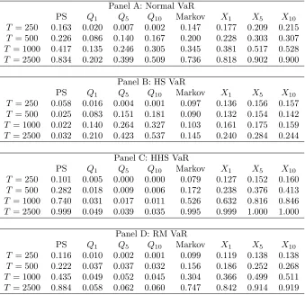
Tables 1–3 report, for each of the testing procedures, the proportion of times (rejection
frequency) a test rejects the null that the VaR model is ‘appropriate’. Since returns are
generated from a GARCH model and quantiles are estimated according to a different model
(Normal, HS, HHS and RM models), the higher the rejection frequency, the better is the
associated test.
Table 1 reports the results for the case when returns are generated according to a GARCH
model with Student-t innovations. For the Normal VaR the proposed Pearson tests based
test across all sample sizes. It is worth stating that the Pearson X1 test shows the same
properties of the Perignon and Smith test. The performance of the Markov test introduced
in the paper is something in between the Pearson and the Perignon and Smith tests, but
better than the Hurlin and Tokpavi test. The results for the Normal VaR are confirmed
by those in Panel C (HHS VaR) and Panel D (RM VaR). For the case of HS VaR (Panel
B) when m = 1 the Pearson test is better than the corresponding Q test. For m = 5 and
m= 10 the Pearson tests outperform the corresponding Qtests in small sample.
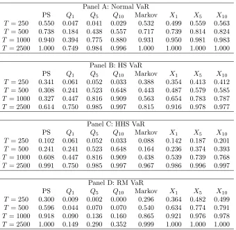
Tables 2 and 3 report the size-adjusted powers of the different test for the case when
returns are generated according to a GARCH model with Skew Student-t and with GED
innovations, respectively.
If we compare the results in Tables 2–3 with those in Table 1, we notice a substantial
increase in power mainly due to the fact that the underlying distributions (skew-t and GED)
make the misspecification in VaR modelling easier to be captured by the tests.
For the case where the Normal distribution is used for computing VaR, i.e. Panel A of
Tables 2 and 3, the Pearson tests we propose in this paper, based on m = 5 and m = 10,
outperform both the Perignon and Smith and Hurlin and Tokpavi tests across all sample
sizes. When T = 2500 all tests but the Hurlin and Tokpavi show the same performance. As
in Table 1, the results of Panels C and D (HHS and RM VaR, respectively) of both tables are
in line with those of Panel A. In Panel B, instead, the best performance is achieved by the
Q10 statistic which is marginally better for T larger than 500, while for T = 2500 all tests
have the same performance. It is worth noticing that the Pearson tests are always better in
terms of power than all the other tests whenT = 250, which is the most common sample size
used in practice. Finally, from the Monte Carlo experiments we can draw useful information
Table 1: Size-adjusted rejection frequencies of multilevel tests at the 5% nominal level and vector of critical levels (1%,2.5%,5%). PS denotes the Perignon and Smith (2008) test, Qm,
m ∈ {1,5,10}, is the Hurlin and Tokpavi (2006) test, Markov is the test (14) and Xm, m ∈
{1,5,10}, is the Pearson test based on (15). Returns are generated according to a GARCH model with Student-t innovations.
Panel A: Normal VaR
PS Q1 Q5 Q10 Markov X1 X5 X10
T = 250 0.163 0.020 0.007 0.002 0.147 0.177 0.209 0.215
T = 500 0.226 0.086 0.140 0.167 0.200 0.228 0.303 0.307
T = 1000 0.417 0.135 0.246 0.305 0.345 0.381 0.517 0.528
T = 2500 0.834 0.202 0.399 0.509 0.736 0.818 0.902 0.900 Panel B: HS VaR
PS Q1 Q5 Q10 Markov X1 X5 X10
T = 250 0.058 0.016 0.004 0.001 0.097 0.136 0.156 0.157
T = 500 0.025 0.083 0.151 0.181 0.090 0.132 0.154 0.142
T = 1000 0.022 0.140 0.264 0.327 0.103 0.161 0.175 0.159
T = 2500 0.032 0.210 0.423 0.537 0.145 0.240 0.284 0.244 Panel C: HHS VaR
PS Q1 Q5 Q10 Markov X1 X5 X10
T = 250 0.101 0.005 0.000 0.000 0.079 0.127 0.152 0.160
T = 500 0.282 0.018 0.009 0.006 0.172 0.238 0.376 0.413
T = 1000 0.740 0.031 0.017 0.011 0.526 0.632 0.816 0.846
T = 2500 0.999 0.049 0.039 0.035 0.995 0.999 1.000 1.000 Panel D: RM VaR
PS Q1 Q5 Q10 Markov X1 X5 X10
T = 250 0.116 0.010 0.002 0.001 0.099 0.119 0.138 0.138
T = 500 0.222 0.037 0.037 0.032 0.156 0.186 0.252 0.268
T = 1000 0.435 0.049 0.052 0.045 0.304 0.366 0.499 0.511
Table 2: Size-adjusted rejection frequencies of multilevel tests at the 5% nominal level and vector of critical levels (1%,2.5%,5%). PS denotes the Perignon and Smith (2008) test, Qm,
m ∈ {1,5,10}, is the Hurlin and Tokpavi (2006) test, Markov is the test (14) and Xm, m ∈
{1,5,10}, is the Pearson test based on (15). Returns are generated according to a GARCH model with Skew Student-tinnovations.
Panel A: Normal VaR
PS Q1 Q5 Q10 Markov X1 X5 X10
T = 250 0.550 0.047 0.041 0.029 0.532 0.499 0.559 0.563
T = 500 0.738 0.184 0.438 0.557 0.717 0.739 0.814 0.824
T = 1000 0.940 0.394 0.775 0.880 0.931 0.950 0.981 0.983
T = 2500 1.000 0.749 0.984 0.996 1.000 1.000 1.000 1.000 Panel B: HS VaR
PS Q1 Q5 Q10 Markov X1 X5 X10
T = 250 0.341 0.061 0.052 0.033 0.388 0.354 0.413 0.412
T = 500 0.308 0.241 0.523 0.648 0.443 0.487 0.579 0.585
T = 1000 0.327 0.447 0.816 0.909 0.563 0.654 0.783 0.787
T = 2500 0.614 0.750 0.985 0.997 0.815 0.916 0.978 0.977 Panel C: HHS VaR
PS Q1 Q5 Q10 Markov X1 X5 X10
T = 250 0.102 0.061 0.052 0.033 0.088 0.142 0.187 0.201
T = 500 0.241 0.241 0.523 0.648 0.164 0.236 0.374 0.393
T = 1000 0.608 0.447 0.816 0.909 0.438 0.539 0.739 0.768
T = 2500 0.991 0.750 0.985 0.997 0.967 0.986 0.996 0.997 Panel D: RM VaR
PS Q1 Q5 Q10 Markov X1 X5 X10
T = 250 0.300 0.009 0.002 0.000 0.296 0.364 0.482 0.499
T = 500 0.596 0.044 0.070 0.070 0.540 0.634 0.774 0.791
T = 1000 0.918 0.090 0.136 0.160 0.865 0.921 0.976 0.978
Table 3: Size-adjusted rejection frequencies of multilevel tests at the 5% nominal level and vector of critical levels (1%,2.5%,5%). PS denotes the Perignon and Smith (2008) test, Qm,
m ∈ {1,5,10}, is the Hurlin and Tokpavi (2006) test, Markov is the test (14) and Xm, m ∈
{1,5,10}, is the Pearson test based on (15). Returns are generated according to a GARCH model with GED innovations.
Panel A: Normal VaR
PS Q1 Q5 Q10 Markov X1 X5 X10
T = 250 0.481 0.064 0.056 0.040 0.465 0.432 0.491 0.492
T = 500 0.601 0.220 0.497 0.622 0.618 0.631 0.723 0.731
T = 1000 0.823 0.429 0.801 0.899 0.844 0.870 0.940 0.946
T = 2500 0.995 0.761 0.988 0.998 0.992 0.998 1.000 1.000 Panel B: HS VaR
PS Q1 Q5 Q10 Markov X1 X5 X10
T = 250 0.328 0.063 0.057 0.038 0.381 0.357 0.419 0.424
T = 500 0.287 0.255 0.552 0.672 0.444 0.490 0.584 0.590
T = 1000 0.325 0.460 0.831 0.923 0.571 0.668 0.800 0.801
T = 2500 0.636 0.779 0.990 0.999 0.838 0.933 0.983 0.983 Panel C: HHS VaR
PS Q1 Q5 Q10 Markov X1 X5 X10
T = 250 0.115 0.007 0.001 0.000 0.104 0.169 0.233 0.247
T = 500 0.271 0.029 0.031 0.032 0.185 0.268 0.431 0.456
T = 1000 0.660 0.063 0.077 0.078 0.505 0.611 0.796 0.824
T = 2500 0.995 0.118 0.198 0.241 0.981 0.993 0.999 0.999 Panel D: RM VaR
PS Q1 Q5 Q10 Markov X1 X5 X10
T = 250 0.144 0.012 0.004 0.001 0.167 0.224 0.286 0.291
T = 500 0.239 0.066 0.098 0.109 0.242 0.322 0.430 0.438
T = 1000 0.480 0.109 0.182 0.211 0.437 0.548 0.707 0.712
in Tables 2–3, we notice an increase in power moving from m = 1 to m = 5, whereas the
increase in power moving from m = 5 to m = 10 is only marginal. Thus we suggest using
m= 5 in practical applications.
4
Empirical application
In this section, we use the full set of multilevel tests for a comprehensive backtesting exercise.
The aim is to illustrate the implementation of the different tests, and to show how they can
deliver contrasting conclusions.
We use daily returns on 15 MSCI world indices traded as iShares on the American
Exchange for the following countries: US, Mexico, Canada, the UK, the Switzerland, Sweden,
Spain, Italy, Germany, France, Australia, Singapore, Japan, Hong Kong and Malaysia. The
exchange traded funds (ETF) do not suffer from problems related to non-synchronicity and
different closing times, unlike the raw indices which trade at different times around the world.
The data covers the period December 2000 to November 2011 (2750 observations).
4.1
Univariate models
First, we consider, in an out-of-sample exercise, the following univariate VaR models: HS,
RM, GARCH and GARCH-t (both with and without an AR(1) model for the mean), HHS,
Filtered Historical Simulation (FHS), and GJR and GJR-t (both with and without an AR(1)
model for the mean). The order of all the GARCH and GJR models is (1,1). For all the
VaR models, with the exception of HS, we use a rolling window of 250 observations, for
both parameters estimation and VaR calculation. Consequently, we end up with 2500 VaR
an expanding window with the first one comprising the first 250 observations, obtaining the
same number of VaR estimates and relative to the same period as the alternative methods.
In Table 4, we report some representative results for a limited number of countries, i.e.
Australia, Germany, USA, and Singapore4. The table reports the p-values for the multilevel
tests based on coverage probabilities 5%, 2.5%, and 1%. For Australia, the Hurlin and
Tokpavi tests do not reject the null in all cases but HS, GARCH and GARCH-t in contrast
to the finding from the Pearson tests that systematically reject the null. For Singapore,
there is evidence of non-contradiction between tests for the case of AR(1)-GARCH-t and
AR(1)-GJR-t only; in all the other cases the Q1, Q5 and Q10 accept the null whereas all
other tests lead to a rejection. The same applies for USA, where however the two models
dominate but in a weaker form than the Singapore case. In addition for USA, the Q1 test
systematically accepts the null with the only exception of the HHS and GJR models. For
Germany, once again all tests do not reject the null only in the AR(1)-GJR-t case. The
HHS model is strongly rejected by all tests with the exeption of the Hurlin and Tokpavi
tests. With respect to the results we do not report in the paper, we mention that
GARCH-t models perform beGARCH-tGARCH-ter GARCH-than GARCH models wiGARCH-th normal innovaGARCH-tions and GARCH-the inclusion
of the mean component (AR(1)-GARCH, AR(1)-GARCH-t, AR(1)-GJR and AR(1)-GJR-t
models) generally improves upon GARCH models without the mean.
4.2
Multivariate models
Next, we estimate the VaR measures in a Multivariate GARCH (MGARCH) context for an
equally weighted portfolio comprising the 15 securities. The motivation for including such
an analysis is that modeling the dependence among returns should improve VaR forecasting.
Table 4: Backtesting Results. The table reports the calculated p-values of the different multilevel tests with vector of probability levels (1%,2.5%,5%) under different VaR models.
AR(1)- AR(1)- AR(1)-
AR(1)-HS RM GARCH GARCH-t GARCH GARCH-t HHS FHS GJR GJR-t GJR GJR-t PS 0.188 0.002 0.000 0.000 0.000 0.098 0.000 0.276 0.000 0.000 0.000 0.021
Q1 0.004 0.039 0.032 0.035 0.421 0.256 0.707 0.287 0.361 0.071 0.304 0.646
Q5 0.000 0.041 0.015 0.005 0.143 0.122 0.489 0.073 0.713 0.167 0.488 0.628
Q10 0.000 0.069 0.005 0.005 0.053 0.035 0.317 0.011 0.766 0.270 0.578 0.432 Australia -EWA Markov 0.004 0.005 0.000 0.000 0.000 0.096 0.000 0.421 0.000 0.000 0.000 0.077
X1 0.001 0.003 0.000 0.000 0.000 0.124 0.002 0.162 0.000 0.000 0.000 0.040
X5 0.000 0.001 0.000 0.000 0.000 0.035 0.000 0.054 0.000 0.000 0.000 0.009
X10 0.000 0.001 0.000 0.000 0.000 0.029 0.000 0.039 0.000 0.000 0.000 0.006
PS 0.096 0.070 0.420 0.400 0.114 0.955 0.000 0.000 0.019 0.064 0.008 0.190
Q1 0.001 0.038 0.087 0.079 0.181 0.083 0.422 0.013 0.005 0.011 0.152 0.256
Q5 0.000 0.002 0.004 0.001 0.002 0.000 0.484 0.000 0.007 0.023 0.293 0.474
Q10 0.000 0.002 0.042 0.007 0.010 0.002 0.606 0.000 0.053 0.135 0.727 0.801 Germany -EWG Markov 0.000 0.019 0.153 0.138 0.090 0.228 0.000 0.000 0.001 0.004 0.008 0.113
X1 0.000 0.004 0.150 0.140 0.077 0.305 0.000 0.000 0.004 0.013 0.021 0.222
X5 0.000 0.002 0.064 0.034 0.011 0.072 0.000 0.000 0.006 0.026 0.009 0.219
X10 0.000 0.004 0.192 0.120 0.035 0.281 0.000 0.000 0.013 0.052 0.014 0.274
PS 0.097 0.012 0.001 0.001 0.004 0.899 0.000 0.030 0.000 0.000 0.001 0.807
Q1 0.243 0.688 0.731 0.725 0.676 0.531 0.381 0.643 0.825 0.813 0.638 0.699
Q5 0.000 0.289 0.469 0.425 0.324 0.070 0.413 0.578 0.937 0.935 0.986 0.865
Q10 0.000 0.335 0.675 0.569 0.326 0.059 0.453 0.106 0.949 0.924 0.761 0.709 Singapore -EWS Markov 0.065 0.039 0.006 0.008 0.016 0.322 0.000 0.052 0.003 0.004 0.003 0.537
X1 0.104 0.051 0.012 0.011 0.029 0.831 0.000 0.076 0.005 0.006 0.007 0.851
X5 0.000 0.005 0.002 0.002 0.006 0.396 0.000 0.017 0.001 0.002 0.002 0.896
X10 0.000 0.005 0.002 0.002 0.004 0.498 0.000 0.006 0.001 0.001 0.001 0.771
PS 0.033 0.001 0.016 0.056 0.027 0.288 0.000 0.003 0.000 0.001 0.001 0.016
Q1 0.003 0.153 0.257 0.074 0.411 0.901 0.037 0.288 0.205 0.368 0.913 0.856
Q5 0.000 0.075 0.041 0.019 0.069 0.149 0.047 0.026 0.479 0.442 0.774 0.852
Q10 0.000 0.020 0.012 0.010 0.014 0.060 0.104 0.004 0.708 0.571 0.775 0.689 USA -SPY Markov 0.000 0.001 0.057 0.032 0.069 0.652 0.000 0.031 0.000 0.003 0.006 0.078
X1 0.000 0.001 0.016 0.021 0.042 0.506 0.000 0.004 0.001 0.003 0.003 0.052
In all cases we estimate an Asymmetric Dynamic Conditional Correlation (ADCC) model
under the multivariate normal assumption (see Cappiello et al., 2006).
In Panel A of Table 5, we report the results for the equally-weighted portfolio of the
15 countries using the univariate VaR models of Tables 4. There is evidence that the PS
test favors the AR(1)-GARCH-t model while all other tests confirm the dominance of the
AR(1)-GJR-t model. The HS model is consistently rejected by all the test employed. The
RM and FHS models are rejected by all the testing procedures with the exception of the
Markov and Hurlin and Tokpavi tests. Finally, the HHS model is always rejected with the
exception of the Markov, X1 and Hurlin and Tokpavi tests. Again, the Q1 test does not
reject any model.
Panel B of Table 5 reports the results for Gaussian MGARCH models. We consider four
different models for the first stage, i.e. GJR with normal (GJR-N) or Student-t innovations
(GJR-t) with and without an AR(1) process for the mean. In all the four cases we fit
a GJR(1,1) model in the first stage and an ADCC(1,1,1) in the second stage. Contrary
to the univariate results, the inclusion of the mean makes the results worse. The GJR-t
model dominates all the other models because it is only rejected by the X10 test at the 5%
confidence level, but not at the the 1% confidence level. Contrary to all the other testing
procedures, the Hurlin and Tokpavi tests are in favour of all the four multivariate compared
in the exercise.
5
Concluding remarks
In this paper, we proposed novel independence and conditional coverage tests in a multilevel
Table 5: Backtesting Results for an equally weighted portfolio of the 15 securities. The table reports the calculated p-values of the different multilevel tests with vector of probability levels (1%,2.5%,5%) under different VaR models.
Panel A: Univariate Models
AR(1)- AR(1)- AR(1)-
AR(1)-HS RM GARCH GARCH-t GARCH GARCH-t HHS FHS GJR GJR-t GJR GJR-t
PS 0.003 0.015 0.015 0.140 0.014 0.543 0.026 0.016 0.002 0.039 0.002 0.249
Q1 0.015 0.626 0.956 0.389 0.870 0.093 0.785 0.346 0.811 0.799 0.706 0.713
Q5 0.000 0.392 0.167 0.229 0.329 0.030 0.212 0.164 0.642 0.749 0.918 0.878
Q10 0.000 0.217 0.006 0.020 0.034 0.000 0.164 0.071 0.296 0.402 0.613 0.550 Markov 0.000 0.110 0.209 0.284 0.130 0.282 0.128 0.061 0.023 0.198 0.010 0.332
X1 0.000 0.044 0.083 0.089 0.063 0.159 0.107 0.021 0.010 0.108 0.007 0.347
X5 0.000 0.005 0.003 0.040 0.003 0.149 0.023 0.003 0.001 0.039 0.002 0.261
X10 0.000 0.003 0.001 0.021 0.002 0.071 0.026 0.003 0.001 0.023 0.001 0.145
Panel B: Gaussian MGARCH Models
GJR N-ADCC GJR t-ADCC AR-GJR N-ADCC AR-GJR t-ADCC
PS 0.024 0.186 0.012 0.038
Q1 0.834 0.746 0.491 0.632
Q5 0.524 0.165 0.451 0.650
Q10 0.119 0.048 0.111 0.039
Markov 0.185 0.490 0.021 0.109
X1 0.083 0.310 0.026 0.079
X5 0.018 0.058 0.004 0.023
X10 0.008 0.044 0.002 0.005
presence of small samples. In risk management analysis, it is practice to estimate quantiles
for two or more different probability levels. To this purpose, using a multilevel test is
intuitively more efficient, and statistically more powerful, than to use separate unilevel tests.
Moreover, multilevel tests are particularly useful because they make the best use of the
limited amount of information regarding the return distribution made available by banks or
financial institutions in general to assess their risk exposure.
The first test we proposed is a generalization to the multilevel case of the Markov test
of Christoffersen (1998), while the second test is a Pearson-type of test based on the joint
distribution of the total number of VaR violations in a period and its lags. In an extensive
Monte Carlo exercise, where returns were generated under alternative GARCH models with
skewed and leptokurtic innovations (i.e. Student-t, skew-t and GED innovations), and where
VaR were estimated using models commonly used in practice (i.e. Normal, HS, HHS and
RM), the multilevel tests we proposed showed higher power than both the multilevel
uncon-ditional test of Perignon and Smith (2008) and the multilevel conuncon-ditional tests of Hurlin and
Tokpavi (2006). Via an empirical application using daily returns on 15 MSCI world indices,
we implemented all available multilevel tests and we showed that in most cases different tests
deliver different conclusions.
Appendix: Maximum likelihood estimators of
π
iand
π
i,jLet us write the log-likelihood function (7) as
ℓ(π) =
K
X
i=0
Tiln(πi) =Tjln(πj) +
X
i6=j
Tiln(πi) = Tjln 1−
X
h6=j
πh
!
+X
i6=j
Tiln(πi),
Setting the derivative w.r.t. πi, i6=j, equal to zero yields
Tjπi =Ti 1−
X
h6=j
πh
!
.
Since the quantity in brackets is equal to πj, the first order conditions are
Tjπi =Tiπj, i= 0, . . . , K, i 6=j.
Summing both sides for every i6=j yields
Tj
X
i6=j
πi =πj
X
i6=j
Ti =⇒ Tj(1−πj) = πj(T −Tj) =⇒ πbj =
Tj
T .
Similarly, let us write (11) as
ℓ(Π) = K
X
i=0
"
Ti,jln(πi,j) +
X
h6=j
Ti,hln(πi,h)
# = K X i=0 "
Ti,jln 1−
X
h6=j
πi,h
!
+X
h6=j
Ti,hln(πi,h)
#
.
Setting the derivative w.r.t. πi,l, i= 0, . . . , K, l6=j, equal to zero yields
Ti,jπi,l=Ti,l 1−
X
h6=j
πi,h
!
=Ti,lπi,j,
since 1−Ph6=jπi,h =πi,j.
Summing over l = 0, . . . , K,l 6=j yields
Ti,j
X
l6=j
πi,l=πi,j
X
l6=j
Ti,l =⇒ Ti,j(1−πi,j) = πi,j(Ti−Ti,j) =⇒ bπi,j =
Ti,j
Ti
Acknowledgements
We wish to thank the Editor, Dick Van Dijk, and an anonymous Referee for very useful
comments and suggestions which greatly helped to improve the content and the presentation
of the paper. The usual disclaimer applies. This paper was completed while Arturo Leccadito
and Simona Boffelli were visiting the Centre for Econometric Analysis of Cass Business School
in January-July 2012. Financial support from the Centre for Econometric Analysis and the
2012 Cass Business School Pump-Priming grant scheme is gratefully acknowledged.
References
Artzner, P., F. Delbaen, and J.-M. E. D. Heath (1999). Coherent measures of risk. Mathematical Fi-nance 9(3), 203–228.
Berkowitz, J. (2001). Testing density forecasts, with applications to risk management. Journal of Business & Economic Statistics 19(4), 465–74.
Berkowitz, J., P. Christoffersen, and D. Pelletier (2011). Evaluating Value-at-Risk models with desk-level data. Management Science 57(12), 2213–2227.
Boudoukh, J., M. Richardson, and R. F. Whitelaw (1998). The best of both worlds: A hybrid approach to calculating Value at Risk. Risk 11, 64–67.
Box, G. E. P. and D. A. Pierce (1970). Distribution of residual autocorrelations in autoregressive-integrated moving average time series models.Journal of the American Statistical Association 65(332), 1509–1526. Box, G. E. P. and G. C. Tiao (1992). Bayesian Inference in Statistical Analysis. New York: Wiley.
Candelon, B., G. Colletaz, C. Hurlin, and S. Tokpavi (2011). Backtesting value-at-risk: A GMM duration-based test. Journal of Financial Econometrics 9(2), 314–343.
Cappiello, L., R. F. Engle, and K. Sheppard (2006). Asymmetric dynamics in the correlations of global equity and bond returns. Journal of Financial Econometrics 4(4), 537–572.
Christoffersen, P. F. and D. Pelletier (2004). Backtesting Value-at-Risk: A duration-based approach.Journal of Financial Econometrics 2(1), 84–108.
Diebold, F. X., T. A. Gunther, and A. S. Tay (1998). Evaluating density forecasts with applications to financial risk management. International Economic Review 39(4), 863–883.
Dufour, J.-M. (2006). Monte Carlo tests with nuisance parameters: A general approach to finite-sample inference and nonstandard asymptotics. Journal of Econometrics 133(2), 443–477.
Engle, R. F. and S. Manganelli (2004). CAViaR: Conditional autoregressive value at risk by regression quantiles. Journal of Business & Economic Statistics 22(4), 367–381.
Hansen, B. E. (1994). Autoregressive conditional density estimation.International Economic Review 35(3), 705–730.
Hurlin, C. and S. Tokpavi (2006). Backtesting value-at-risk accuracy: a simple new test.Journal of Risk 9(2), 19–37.
Kupiec, P. H. (1995). Techniques for verifying the accuracy of risk measurement models. Journal of Deriva-tives 3, 73–84.
Li, W. K. and A. McLeod (1981). Distribution of the residual autocorrelations in multivariate ARMA time series models. Journal of the Royal Statistical Society, Series B 43(2), 231–239.
Arturo Leccadito (Ph.D., Bergamo) is Assistant Professor of financial mathematics at the
De-partment of Economics, Statistics and Finance of the University of Calabria, Italy. His research
interests include financial econometrics, credit risk modelling and option pricing. He has published
in Quantitave Finance, Econometric Reviews and International Journal of Theoretical and Applied
Finance, and others.
Simona Boffelli (MSc., Bergamo) is a PhD candidate at the University of Bergamo, Italy. Her
research interests are in financial econometrics, modelling risk and cross-market correlations, asset
pricing, modelling jumps and cojumps and the impact of macrofactors, macronews, bond auctions
and credit rating actions on European bond markets.
Giovanni Urga (Ph.D., Oxford) is Professor of Finance and Econometrics and Director of the
Centre for Econometric Analysis (CEA@Cass) at Cass Business School, London, U.K., and
pro-fessor of Econometrics at the University of Bergamo, Italy. His research interests are in panel
data, financial econometrics, modelling risk and cross-market correlations, asset pricing, structural
breaks, modelling common stochastic trends, and credit spreads. He has published in the Journal
of Econometrics, Journal of Business and Economic Statistics, Economics Letters, Econometric
Theory, Oxford Bulletin of Economics and Statistics, Journal of Applied Econometrics,
Interna-tional Journal of Forecasting, and others. He is an Associate Editor for Empirical Economics, and
has been a guest editor for the Journal of Econometrics and the Journal of Business and Economic