Wavelet-Based Characterization and Stochastic Modelling of Pulse-like Ground Motions on the Time-frequency Plane

(1)

City, University of London Institutional Repository

Citation

:

Lungu, A. (2014). Wavelet-Based Characterization and Stochastic Modelling of Pulse-like Ground Motions on the Time-frequency Plane. (Unpublished Doctoral thesis, City University London)

This is the accepted version of the paper.

This version of the publication may differ from the final published

version.

Permanent repository link:

http://openaccess.city.ac.uk/8341/

Link to published version

:

Copyright and reuse:

City Research Online aims to make research

outputs of City, University of London available to a wider audience.

Copyright and Moral Rights remain with the author(s) and/or copyright

holders. URLs from City Research Online may be freely distributed and

linked to.

City Research Online: http://openaccess.city.ac.uk/ [email protected]

(2)

WAVELET-BASED CHARACTERIZATION AND

STOCHASTIC MODELLING OF PULSE-LIKE GROUND

MOTIONS ON THE TIME-FREQUENCY PLANE

by

Anca Lungu

Dissertation submitted in fulfilment of the requirements for the award of

DOCTOR OF PHILOSOPHY

in

STRUCTURAL ENGINEERING

School of Engineering and Mathematical Sciences City University London

(3)

LIST OF TABLES

Table 4.1. Correlation coefficients ... 58

Table 5.1. Parameters for the simulation of the Imperial Valley accelerogram... 97

Table 5.2. Parameters for defining the HF content compatible with EC8 spectrum... 101

Table 6.1. Parameters for defining pulse processes ... 107

Table 6.2. Frequency dependant level of resolution ... 110

Table 6.3 Mean value and standard deviation of the correlation coefficients ... 123

(8)

LIST OF FIGURES

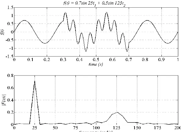
Figure 2.1. Superposition of two sinusoids and the FT magnitude spectrum ... 8

Figure 2.2.The effect of the fixed width window function ... 10

Figure 2.3. Spectrogram of a signal ... 9

Figure 2.4. Time-domain and frequency domain representation of wavelet functions ... 13

Figure 2.5. Wavelet transform of a signal ... 13

Figure 2.6. Wavelet tree for DWT(left) and for WPT (right) ... 21

Figure 2.7. Generalized harmonic wavelets at different scales ... 22

Figure 2.8. Generalized harmonic wavelet basis... 22

Figure 2.9. Discrete GHWT (left) and continuous GHWT (right)... 23

Figure 2.10. Meyer wavelet: time domain and frequency domain representation ... 24

Figure 2.11. The difference between the S-wavelet and the Morlet wavelet ... 26

Figure 2.12. Intrinsic mode functions (IMFs) of a signal ... 28

Figure 2.13. Empirical mode decomposition scheme ... 29

Figure 3.1. Non-pulse ground motion versus pulse- like ground motion ... 34

Figure 3.2. Schematization of the forward directivity effect (planar view) ... 35

Figure 3.3. Parameters commonly employed for pulse characterization ... 37

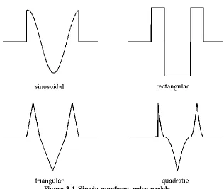
Figure 3.4. Simple waveform pulse models ... 40

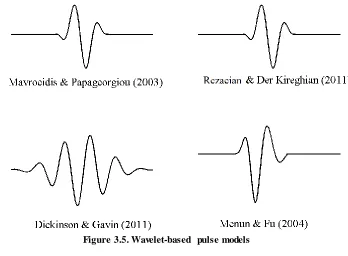
Figure 3.5. Wavelet-based pulse models... 42

Figure 4.1. Filtered accelerograms and the corresponding velocity traces (I) ... 61

Figure 4.2. Filtered accelerograms and the corresponding velocity traces (II) ... 62

(9)

List of figures Figure 4.4. Time-frequency representations for an accelerogram reasonably corrupted

with higher frequency components ... 64

Figure 4.5. Application of the proposed non-separable non-stationary stochastic pulse-like ground motion model for the special case of P = R = 1 ... 66

Figure 4.6. Power spectra shapes for representing the broadband frequency content .... 68

Figure 4.7. The BGB envelope function ... 69

Figure 4.8. Power spectrum density shapes for the pulse content... 69

Figure 4.9. Time-varying envelope for the pulse part... 71

Figure 4.10. Methodology for generating artificial pulse- like accelerogram ... 73

Figure 5.1 Daubechies wavelet function of order 4 (Db4)... 76

Figure 5.2. Histograms of the bandwidth and dominant frequencies of the pulses ... 77

Figure 5.3. Envelopes estimated for pulses... 79

Figure 5.4. Analytic envelopes for various values of γ ... 82

Figure 5.5. Initial quality of matching of spectral ordinates across the database ... 84

Figure 5.6. Comparison between alternative pulse period definitions ... 85

Figure 5.7. Impact baseline corrections on the response spectra – average match for shot pulses (periods under 4s) ... 88

Figure 5.8. Impact baseline corrections on the response spectra – average match for medium pulses (periods between 4s – 6s) ... 88

Figure 5.9.Impact baseline corrections on the response spectra – average match for long pulses (periods over 6s) ... 89

Figure 5.10. Quality of matching across the database after calibration ... 90

Figure 5.11. Average response spectra across the database considered ... 91

Figure 5.12. Peak ground acceleration, velocity and displacement o f the simulations... 91

Figure 5.13. Arias Intensity and Cumulative absolute velocity for the simulations ... 92

(10)

List of figures

Figure 5.15. Pulse period versus earthquake magnitude ... 94

Figure 5.16. Pulse parameters versus magnitude and closest distance ... 95

Figure 5.17. The instant of the peak occurrence tp ... 95

Figure 5.18. The shape parameter γLF ... 96

Figure 5.19 Acceleration, velocity and displacement time traces for the Imperial Valley record - station El Centro #6 ... 97

Figure 5.20 Sample of the HF+COS process and of the HF + BOX process for the simulation of the Imperial Valley record ... 98

Figure 5.21 Displacement samples of the HF+COS process and HF + BOX process.... 98

Figure 5.22. Elastic response spectra of the HF+BOX and HF+COS processes. Inelastic response spectra of the HF+BOX and HF+COS processes ... 100

Figure 5.23 Response ratio for the HF+COS and HF+BOX processes ... 100

Figure 5.24 Acceleration samples compatible with EC8 ... 102

Figure 5.25. Elastic response spectra for pulse-like EC8 compatible processes. Inelastic response spectra for pulse- like EC8 compatible. ... 102

Figure 6.1. Probability distribution of pulse periods across the database ... 105

Figure 6.2. Statistics for the pulse periods and magnitudes in the database ... 106

Figure 6.3. Assessment of time- frequency representations via the EPSD ... 109

Figure 6.4. Theoretical EPSD for the SCOS process. EPSD estimated via HWT and MWPT. Average TFR using the ST... 111

Figure 6.5. Theoretical EPSD for the SBOX process. EPSD estimated via HWT and MWPT. Average TFR using the ST... 112

Figure 6.6. Theoretical EPSD for the LCOS process. EPSD estimated via HWT and MWPT. Average TFR using the ST... 112

(11)

List of figures Figure 6.8. Identification of the low-frequency and high frequency ridges for the short

processes... 113

Figure 6.9. Identification of the low-frequency and high frequency ridges for the long processes... 114

Figure 6.10. Assessment of time- frequency representations via reconstructed pulses . 116 Figure 6.11. Pulse-like accelerogram (arbitrary sample of the SCOS process) ... 122

Figure 6.12. Pulse-like accelerogram (arbitrary sample of the LBOX process) ... 122

Figure 6.13. SCOS–correlation between LF samples and reconstructed pulses ... 124

Figure 6.14. SBOX–correlation between LF samples and reconstructed pulses ... 124

Figure 6.15. LCOS–correlation between LF samples and reconstructed pulses ... 125

Figure 6.16. LBOX–correlation between LF samples and reconstructed pulses ... 125

Figure 6.17. Average pulse response ratios for the SCOS samples ... 128

Figure 6.18. Average pulse response ratios for the SBOX samples ... 128

Figure 6.19. Average pulse response ratios for the LCOS samples ... 129

Figure 6.20. Average pulse response ratios for the LBOX samples ... 129

Figure 6.21 1971 San Francisco (Pacoima Dam)... 133

Figure 6.22 1971 San Francisco: reconstructed pulses ... 133

Figure 6.23 1971 San Francisco: spectral responses for ductility factor μ = 1 & 2 ... 134

Figure 6.24 1971 San Francisco: spectral responses for ductility factor μ = 4 & 8 ... 134

Figure 6.25 1994 Northridge (Rinaldi). ... 135

Figure 6.26. 1994 Northridge: reconstructed pulses ... 135

Figure 6.27 1994 Northridge: spectral responses for ductility factor μ = 1 & 2 ... 136

Figure 6.28 1994 Northridge spectral responses for ductility factor μ = 4 & 8 ... 136

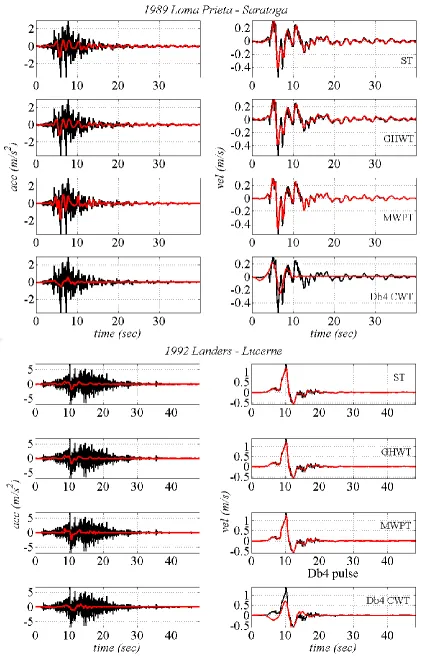
Figure 6.29 1989 Loma Prieta (Saratoga) ... 137

Figure 6.30 1989 Loma Prieta: reconstructed pulses ... 137

(12)

List of figures

Figure 6.32 1989 Loma Prieta spectral responses for ductility factor μ = 4 & 8 ... 138

Figure A.1 Frequency domain interpretation of the time-domain integration...147

Figure A.2 High-pass Butterworth filter ... 148

(13)

ACKNOWLEDGMENTS

I would like to express my sincerest gratitude to my supervisor Dr Agathoklis Giaralis

for his continuous support, patience and encouragement. I was very lucky to find in him a devoted mentor always open to listening and discussing any questions that arose in the course of my studies. His perpetual commitment, selfless time and professionalism were essential for the completion of this thesis.

I would also like to thank the members of staff of the School of Engineering and Mathematical Sciences Department for valuable advice and support throughout the teaching activities I have undertaken.

I am grateful to City University London for the financial support offered throughout my studies. The partial support of the School of Engineering and Mathematical Sciences Department is also gratefully acknowledged.

I am truly thankful to Professor Pavel Alexa for advising me and opening the routes towards my doctoral education.

(14)

Acknowledgments I cannot express in words my appreciation towards Persida Fira-Mladinescu who was like a mother to me during all these years, Iulia Muntean for her unceasing guidance and warm support and Alexandra Crişan for keeping me optimistic and brave.

A deep and heartfelt thank you to my sister Silvia Bashir, one of my main pillars, for her never ending support and unconditional love which kept me harmonious and equilibrated throughout this journey. I warmly thank my sister‟s family who embraced me with open hearts and offered me amazing holidays.

(15)

DECLARATION

(16)

ABSTRACT

A novel non-separable non-stationary stochastic model for the representation and simulation of pulse-like earthquake ground motions (PLGMs), capable to accurately represent peak elastic and inelastic structural responses, is proposed in this work. Further, the model is employed for assessing the performance of several time-frequency representation techniques (the harmonic wavelet transform, the Meyer wavelet packets transform, the S-transform and the empirical mode decomposition) in capturing salient features of pulse-like accelerograms.

The significantly higher structural demands posed by PLGMs in comparison with similar intensity pulse-free motions led to comprehensive investigations in order to mitigate the damage experienced in the affected areas, such as those located near seismic faults. In this regard, time-frequency analysis methods are frequently employed for the analysis of signals recorded during these events, due to their adaptability to the specific evolutionary behaviour. Alongside with characterization, stochastic modelling of PLGMs is of interest since it allows for systematic variations of the input parameters in order to enhance the understanding of their influence on the structural behaviour. This is particularly useful since only a limited number of PLGMs are available in the existing earthquake databases.

Accordingly, inspired by the time-frequency distribution of their total energy, a versatile PLGM model is defined as a combination of amplitude-modulated stochastic processes. Each process models the time-varying distribution of the energy for adjacent frequency ranges. Two alternative formulations are proposed for representing the low-frequency content characterizing the pulses. Considering a set of pulses from the literature, numerical results show that the pulse models‟ parameters can be calibrated to simulate in average the structural impact of these pulses represented using the model herein defined. Further, the capability of the PLGM model to generate elastic and inelastic spectral responses matching a given field recorded accelerogram in the mean sense is illustrated. The applicability of the proposed model to account for near-fault effects to spectrum compatible representations of the seismic action is illustrated by generating a fully stochastic process compatible with the response spectrum of the European aseismic code (EC8). Furthermore, the model can be employed in various applications including generation of accelerograms for nonlinear dynamic analyses of structures, probabilistic seismic demand analyses or as input in stochastic dynamic techniques such as statistical linearization.

(17)

CHAPTER 1 :

INTRODUCTION

1.1. MOTIVATION

Signals recorded during pulse-like seismic ground motions (PLGMs) distinguish themselves through the presence of unusually high amplitude, long period oscillations termed as “pulses”. It has been observed that such ground motions have a particularly strong impact on relatively flexible structures, whose dominant fundamental period is close to the pulse period. Consequently an important amount of research was devoted especially in the past two decades to understanding and characterizing such earthquakes, with the aim of improving the structural behaviour in the affected areas. A major limitation of these studies is the modest amount of field recorded data available, which includes less than 100 records being classified in the literature as pulse-type. As a result, the development of record-based stochastic models to be used for various applications is an essential matter in pulse-like ground motions related research.

(18)

Chapter 1 Introduction pulse parameters by considering specific ensembles of records (Bray & Rodriguez-Marek, 2004; Dabaghi et al. 2011; Dickinson & Gavin, 2011).

In this context an alternative stochastic modelling approach inspired by the time-frequency distribution of the record's energy is proposed in this work. It employs a simple but popular representation method to shape the energy distribution of pulse-like ground motions, which has been previously used for various structural dynamics matters (e.g. Conte & Peng, 1997; Spanos & Failla, 2004). The approach consists in superposing several amplitude-modulated random processes, obtaining this way a non-separable, non-stationary random process. Existing stochastic models for the higher frequency content are combined with newly defined ones for pulses. The proposed model aims for simplicity, consistency and flexibility in choosing the level of detailing for the generated processes, while offering a fully stochastic representation of pulse-like ground motions. It is likely that the model will be employed in diverse applications such as performance-based earthquake engineering studies (e.g. Taflanidis & Jia, 2011; Taflanidis, 2011) or statistical linearization-based applications for structural engineering (e.g. Spanos & Giaralis, 2008; Spanos & Kougioutzoglou, 2012).

(19)

Chapter 1 Introduction (three wavelet-based, i.e. the harmonic wavelet, Meyer wavelet packets and S transforms, in addition to the empirical mode decomposition) to identify and isolate the characteristic pulses from pulse-like accelerograms. Two methodologies are developed for this purpose: one has been previously used in the literature for this sort of assessments, while the second one has been developed for the purpose of the herein study in order to exploit the advantages of using controlled-input data.

1.2. THESIS ORGANISATION

This dissertation consists of seven chapters and four appendices, followed by a list of references. The introductory first chapter presents the motivation of the objectives of this research work, followed by an outline of the thesis. The second chapter provides the necessary mathematical background for the signal processing techniques used throughout this work. The advantages and limitations of wavelet-based techniques, together with the main types of wavelet-transform are presented. The generalized harmonic wavelet transform, the Meyer wavelet packets transform, the S-transform and the empirical mode decomposition are revised.

In the third chapter a review of the pulse-like ground motions topic is provided. The distinctive phenomenological features characterizing pulse-like records are exemplified and the physical conditions likely to cause them are presented. Further, the parameters used for the quantification of their characteristics and the pulse models currently existing in the literature are summarized. Finally, the approaches used for the identification and extraction of pulses from the recorded time-histories are reviewed; the currently employed models for modelling and simulating such ground motions are also presented.

(20)

Chapter 1 Introduction presented and the model employed in this work for the higher frequency content representation is described. In the fifth chapter the pulse models are fitted to a given database of pulses. Further, the pulse-like ground motion model is calibrated against a given accelerogram in order to portray its potential in simulating realistic structural elastic and inelastic responses. Additionally, its applicability for incorporating pulse-like effects in code-compatible accelerograms is demonstrated.

In the sixth chapter the techniques used for the characterization of pulse-like records and the identification/extraction of pulses are assessed. In the first part the potential of the generalized harmonic wavelet transform, the Meyer-wavelet packets transform and the S-transform to estimate the underlying energy distribution of pulse-like processes is evaluated. In the latter part, the same techniques, together with the empirical mode decomposition are evaluated by employing them for pulse extraction from artificial accelerograms. Finally, pulses are extracted from several field recorded accelerograms using the approach proposed herein and their quality is assessed in terms of structural responses.

Chapter seven summarizes the main findings presented in this dissertation, acknowledges the limitations of this work and suggests potential future developments.

(21)

CHAPTER 2 :

TIME-FREQUENCY ANALYSIS

TECHNIQUES

2.1. PRELIMINARY REMARKS

(22)

Chapter 2 Time-frequency analysis techniques

2.2. THE FOURIER TRANSFORM

The frequency domain representation of a finite energy signal f (t) is given by the equation

1

ˆ( ) ( )

2

i t

F



f t e dt



 







(2.1)

This conversion from the time-domain to the frequency domain representation is known as the Fourier transform (FT) and is based on the agreement that any periodic function of time can be expressed as an infinite summation of harmonics, with specific amplitude, frequency and phase (Newland, 1984). The frequency content of a signal is thus determined by carrying out its convolution with each decomposing harmonic. High values of the coefficients indicate the presence of the harmonic‟s frequency in the signal. The time domain representation can be recovered by taking the inverse FT given by

 

1 _{ˆ( )}

2

i t

f t F



e d













(2.2)

According to the Parseval‟s theorem the energy of the signal is conserved throughout the transform:

2

2 ˆ

( ) ( )

En f t dt F



d



 

 

(23)

Chapter 2 Time-frequency analysis techniques By treating |f(t)|2 as a probability density function, information on the localization of the signal in time and its duration can be obtained by estimating the time average E[t] and the variance σt as (Cohen, 1995)

 

2

( )

E t t f t dt









(2.4)

 





2 2

 

2 2 2

( )

t t E t f t dt E t E t







 





  _{ } (2.5)

In a similar way, the average frequency E[ω] and the standard deviation σω offer information about the frequency localization and bandwidth of the signal, i.e.:

 

2

ˆ( )

E



 

F d











(2.6)

 





2 2

 

2 ˆ( ) 2 2

E F d E E











 





  _{ } (2.7)

(24)

 

1 1 1 2 2 2

1 1 1

2 2 2

sin

0.7

25 [0,1]

0.5

125 [0.3,0.7]

f t

A

t

A

t

A

t

A

t















(2.8)

[image:24.596.194.490.295.511.2]

Note that the in the Fourier amplitude spectrum (Figure 2.1– bottom panel) shows the frequency components in the signal without any information on their location or duration in time. In case this information is important, the Short Time Fourier Transform can be employed for analysis, as detailed in the following section.

Figure 2.1. Superposition of two sinusoids with different durations and the corresponding FT magnitude spectrum

2.3. THE SHORT TIME FOURIER TRANSFORM

The Short Time Fourier Transform (STFT) computes the FT for successive parts of the signal, delimited by means of a window function w(t). By sliding the window along the time axis using a translation parameter b, a representation of the frequency content of the signal localized in time is obtained as

1

( , ) ( ) ( )

2

i b

STFT t



f b w t b e  db









(25)

Chapter 2 Time-frequency analysis techniques The localization in time is ensured through the following property of the window function w(t):





1

0

for t around b w t b

otherwise

   

 (2.10)

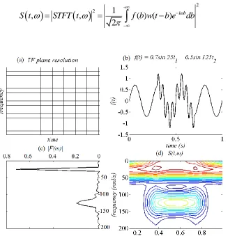
The distribution of the signal energy on the time-frequency plane can be approximated using the STFT by considering the so-called spectrogram, defined as:

 

2 1 2

, , ( ) ( )

2

i b

S t



STFT t



f b w t b e  db









[image:25.596.170.510.277.616.2]

 



 (2.11)

Figure 2.2. Spectrogram of a signal: (a) time-frequency plane discretization; (b) time-domain representation of the signal; (c) Fourier amplitude spectrum; (d) spectrogram of the signal

(26)

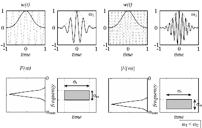
Chapter 2 Time-frequency analysis techniques bandwidth. This dissimilarity is the effect of the resolution (i.e. the level of detail) employed for the representation. The resolution depends on the localization properties of the analysing window w(t), namely the duration (which can be measured using Eq. (2.5)) and the bandwidth of the windowed signal (Eq. (2.7)). Ideally, the smaller σt and

σω, the more accurate is the representation. However, the sizes of these quantities are interdependent and governed by the following equation:

1 2

t 

 

  (2.12)

[image:26.596.160.506.478.698.2]

This dependency, characteristic to all oscillatory functions, implies a trade-off between the resolution in time and in frequency domain and is due to the Heisenberg (or uncertainty) principle (Cohen, 1995). The limitations posed by this principle are very intuitive: if a function is contracted in time (i.e. implying that it has good time localization), its frequency content broadens (i.e. reduced frequency localization); if it is dilated, the frequency content becomes better localized.

(27)

Chapter 2 Time-frequency analysis techniques In the case of the STFT the size of the window is chosen before the analysis and remains fixed at all times and frequencies; the result is a constant resolution across the time-frequency plane (Figure 2.2a). In Figure 2.3 the effect of a constant resolution across the time-frequency representation is exemplified. Note that as the frequency content analysed increases (thus the duration of the oscillations shortens) more oscillations are located in the same time-interval σt, leading to a less accurate localization of their occurrence in time.

The selection of a window-size capable to ensure satisfactory representation of the signal on the time-frequency plane is a challenging issue. This becomes even more critical when dealing with signals characterized by broad frequency content, as it is the case of those encountered in earthquake engineering. The wavelet transform emerged as a technique capable to overcome these limitations by using windows of varying sizes, which adapt to the frequency content being analysed.

2.4. THE WAVELET TRANSFORM

2.4.1. General remarks

(28)

 

,

1

; 0,

b a a

t b

t a b

I_ a







_  _  

  (2.13)

Having a family of wavelets which satisfy specific conditions (detailed in the following section), the representation of the signal on the joint time-frequency plane is obtained by successively performing the inner product with each wavelet in the following way:

 

*

, 1

, _a ( ) _{b a}( )

WT b a f t t dt

I  



 





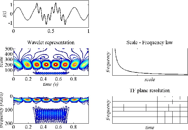
(2.14)

The wavelet transform of the previously considered signal (Eq. (2.8)) can be seen in Figure 2.5. According to the convolution theorem, the following correspondence between the time and frequency domains exists for finite energy functions (Newland, 1984; Cohen, 1995):



_{f g t}

_

 

_

_F

ˆ

   

_

_G

ˆ

_

_(2.15)

where the symbol „*‟ stands for convolution. Consequently, it is less computational demanding to perform the wavelet transform in the frequency domain. Additionally, for scaling the wavelet function, the following relationship exists between the time and the frequency domain (Figure 2.4):

 

ˆ

_,

₀

t

f

a F a

a



  



 

 

(2.16)

(29)

Chapter 2 Time-frequency analysis techniques following relationship between the dominant frequency of the mother wavelet ωc (i.e. the peak of its FT representation) and the frequency of the scaled wavelets (Teolis, 1998; Qian, 2002):

,

b a

c

a





[image:29.596.160.496.162.428.2]



 (2.17)

Figure 2.4. Time-domai n and frequency domain representation of wavelet functions obtained for different scaling factors

[image:29.596.161.485.475.699.2]

(30)

Chapter 2 Time-frequency analysis techniques 2.4.2. Properties for wavelet functions

In order to ensure the reconstruction of the signal from the decomposition, wavelet functions must satisfy the following admissibility condition (Farge, 1992; Teolis, 1998; Qian, 2002; Mallat, 2009):

2

ˆ ( )

C_  d













  (2.18)

where Ψ(ω) is the frequency domain representation of the mother wavelet. Equation (2.18) implies the function has finite energy; for this to be true, the wavelet has to have finite duration in time:

 

t dt







 



(2.19)

A second implication is that the following equation needs to be satisfied as well:

0

ˆ ( )

d



 

 



(2.20)

The integral (2.20) is finite when the function ˆ ( )



decays fast as





0

, which indicates that



 

t

needs to have zero-mean and thus it has to be an oscillatory function:

(0) ( )t dt 0









(31)

Chapter 2 Time-frequency analysis techniques 2.4.3. Wavelet normalization and reconstruction of the decomposed signals

The magnitudes of the WT coefficients obtained at different scales have to be directly comparable, thus appropriate normalization of the wavelets needs to be performed. It is a common practice for the normalization factor

I

a to ensure that wavelets at different scales have unit energy content (L2 normalization) i.e.

2 ₂

,

, ₂

( ) 1

( ) 1, ( ) 0

b a

b a a

t t b

dt dt t a

I a a

           _ _      



(2.22)

This type of normalization (also implemented in the MATLAB Wavelet Toolbox) is appealing since it guarantees the conservation of the signal‟s total energy throughout the transform (Farge, 1992). In this context, the time-scale representation of the signal's energy content distribution, known as the scalogram, can be obtained as

 

2 _* 2

, 1

, , ( ) _{b a}( )

Scal b a WT b a f t t dt

a







 



(2.23)

Further, the signal can be reconstructed from the transform by means of the following equation:

 

2

 

1 ,

t b

f t

C

WT a b

dadb

a

 











_

_







(2.24)

Alternatively, different normalizations of the wavelet function can be performed. The wavelets can be normalized to have unit area (L1 normalization):

,

, ₁

( ) 1

( ) 1, ( ) 0

b a

b a a

t t b

dt dt t a

I_ a a



_

        _ _      

(32)

Chapter 2 Time-frequency analysis techniques or unit amplitude (L∞ norm):

, ( ) 1,( ) 0

b a t a

 _   (2.26)

The type of normalization used for the wavelet function influences the appearance of the time-frequency image of the signal, emphasizing differently the component frequency content, as observed and discussed in the comparative studies such as Farge (1992), Ventosa et al. (2008) or Vassiliou & Makris (2011).

2.4.4. Choice of the analysing wavelet function

The characteristics of the wavelet functions also influence the image of the signal obtained through the decomposition and should be considered when interpreting the resulting representations (Farge, 1992; Torrence & Compo, 1998):

 Complex versus real wavelets

Complex wavelets offer information about the phase and the amplitude which makes them suitable for the analysis of highly oscillatory functions. Real wavelets return information about the amplitude and are useful for identifying peaks or discontinuities in the signals.

 Orthogonal versus non-orthogonal wavelets

Orthogonal wavelets are families of uncorrelated functions, with the zero inner product between any two different functions:

 

1 2 1 2

, , , , , 0, 1 2; ,1 2 0

b a b a b a t b a t dt for a a a a



_







_ _ _



(2.27)

(33)

Chapter 2 Time-frequency analysis techniques independent. The non-orthogonal wavelets lead to over-complete representations, which are suitable for smooth representations of signals.

 Width of the wavelet

The width is relevant in terms of localization of the frequency content in time and frequency. Each wavelet defines a window on the time-frequency plane with the following area (Qian, 2002):



t a t,t a t



,

a a

 

 

    

  _   _

  (2.28)

2a t 2 4 t const

a





 

 

 (2.29)

Although both WT and STFT are subjected to the limitations of the uncertainty principle, the difference between them lays in the fact that the resolution (i.e. level of detail) of the WT representation can be varied according to the range of frequencies analysed (as it can be seen by comparing Figure 2.2 and Figure 2.5), as long as the area of each box delimited by the wavelet on the time-frequency plane remains constant (Figure 2.4).

 Shape of the wavelet

This attribute refers to the smoothness of the function. The choice of the shape depends on the visual appearance of the signal – for smooth signals smooth functions are preferred, while for signals with sharp jumps, other functions might be more appropriate (Daubechies, 1992).

(34)

Chapter 2 Time-frequency analysis techniques the Gaussian (Vassiliou & Makris, 2011; Gupta & Mukhopadhyay, 2013), Meyer wavelets (Yamamoto & Baker, 2013), harmonic wavelets (Spanos & Failla, 2004; Giaralis & Spanos, 2009; Spanos et al., 2009; Spanos & Kougioumtzoglou, 2012).

2.4.5. Types of wavelet transform

There are several ways to perform the WT depending on the scope of the analysis (Daubechies, 1992). The difference between them lies in the values adopted for the scaling and translation parameters and in the characteristics of the mother wavelet. The types of WT used in this work are briefly reviewed herein, while a more comprehensive treatment of this topic can be found in (Daubechies, 1992; Teolis, 1998; Mallat, 2009). The continuous wavelet transform (CWT) is commonly used for achieving smooth representations of the signals on the time-frequency plane. The dilation and translation parameters a and b vary continuously over the time-frequency plane, leading to highly redundant representations, and thus very detailed portrayals of the signal‟s content evolution over the time-frequency plane (see Figure 2.5). The CWT is a computationally demanding technique; its numerical implementation involves considering specific discrete values, whose density determines the resolution of the output.

The discrete wavelet transform (DWT) is a complete and non-redundant version of the WT usually employed for data compression, for modelling purposes or for denoising (Teolis, 1998; Mallat, 2009). The wavelet families used for performing DWT form bases of orthogonal functions. The values of the scaling and translation parameters commonly follow a dyadic sampling, i.e.:

1

, {0}

2 2 ,

i i

a i

b k k

  

 

(35)

Chapter 2 Time-frequency analysis techniques From a numerical implementation point of view, an alternative and more straightforward approach than successively applying Equation (2.14) can be used for obtaining the coefficients of the DWT, namely by using filter banks (see Daubechies, 1992; Mallat, 1989, 2009). Mallat (1989, 2009) showed that the decomposition of a signal on a basis of wavelets consisting of compactly supported functions sampled on a dyadic grid, is similar to a repeated filtering of the signals using conjugate mirror filters (used in filter banks). Based on this property, appropriately chosen filters can be used to decompose a signal on the TF plane, following the methodology detailed further on. Filter banks are used in signal processing for obtaining different level of approximations of the analysed input. The signal is passed through a pair of filters, a low-pass (LP) and high-pass (HP), which separate its content in approximations and details, as it can be seen in the left panel of Figure 2.6. The approximation coefficients (Aji) are the output

of the LP filter and represent averages of the signal. The detail coefficients (Dji)

correspond to the HP filter and represent its oscillatory parts, i.e. the details which are lost through averaging (Mallat, 1989, 2009).

The filtering is performed successively to the output of the LP filter. At each step, the down-sampling (2) of the filtered signal ensures the non-redundancy of the results. The procedure is repeated until the desired level of approximation is obtained. For each level j of the decomposition, the output of the LP filter is Aj+1 = Aj + Dj. This implies that the original signal can be reconstructed by adding up the final output of the LP filter with all the detail coefficients obtained, i.e.:

1

( )

n

n j

j

f t

A

D







(2.31)

(36)

Chapter 2 Time-frequency analysis techniques tree is asymmetric. The number of times the filters are applied gives the depth of the tree. Since in practice we work with discrete-valued signals, the maximum depth of the tree (J) is limited by the total number of samples (discrete points) N in a signal (Mallat, 2009):

2 log

J N (2.32)

There are cases when a more uniform resolution of the TF plane is needed. This can be achieved by applying the wavelet packets transform (WPT), an extended version of the DWT. In this case, not only the approximations of the signal, but also the detail coefficients are further processed until the sought level of approximation is acquired, as shown in the right panel of Figure 2.6. The wavelet tree obtained in this case is symmetrical and just like in the previous case the nodes are orthogonal to each other, encompassing information from adjacent frequency bands. The decomposition is still non-redundant, since the output of each filter and at each level is down-sampled before being further processed. For cases when a more detailed discretization is desired in specific frequency intervals, the output of the corresponding nodes is further processed. From a TF representation perspective, the flexibility of the WPT is important since it offers the opportunity to “zoom-in” within certain frequency bands at will.

(37)

Figure 2.6. Wavelet tree for DWT(left) and for WPT (right)

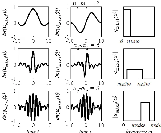
2.4.6. Generalized harmonic wavelet transform

The generalized harmonic wavelets (GHW), introduced by Newland (1994), are complex functions characterized by a box-like shape in the frequency domain. Their frequency support is defined by means of two parameters: the lower limit m and the upper limit n (see Figure 2.7). The Fourier domain representation of GHW at scale (m, n) and located at the time instant b is given by the formula:

 

,

1

, 2 2 ,

2 ( )

0, ˆ

b

m n

m n n m

n m

otherwise











_    

 (2.33)

(38)

[image:38.596.199.458.64.278.2]

Figure 2.7. Generalized harmonic wavelets at different scales

Figure 2.8. Generalized harmonic wavelet basis

(39)

Chapter 2 Time-frequency analysis techniques The GHWs are used in the following chapters in a CWT context, in order to obtain a complete and detailed characterization of the signals (Newland, 1999). To obtain the CWT, the Fourier product between each wavelet and the signal is padded with zeros until the entire frequency axis is covered, before taking the IFFT to obtain the wavelet transform coefficients (Figure 2.9 - right panel). The zero-padding of the frequency domain product between the signal and the wavelet is equivalent with an interpolation between the coefficients for the intermediate time instants, leading to a smoother and more detailed image of the signal‟s content (Newland, 1999).

Due to the flexibility in adjusting the resolution of the TF representation, the GHWs have been used in seismic related applications, i.e. for power spectrum estimation (Spanos & Failla, 2004; Spanos & Kougioumtzoglou, 2012) or for response spectrum matching modification (Giaralis & Spanos, 2009; Spanos et al., 2009).

Figure 2.9. Discrete GHWT (left) and continuous GHWT (right)

2.4.7. Meyer wavelet packets transform

(40)

Chapter 2 Time-frequency analysis techniques filters and form bases, although overlapping exists between adjacent scales (Daubechies, 1992; Mallat, 2009). The Fourier transform of MW is defined as

 

2

1 3 2 4

sin 1 ,

2 2 3 3

2

1 3 4 4

ˆ cos 1 , ,

2 4 3 3

2 0, i i e e otherwise  



_

_



_



 







   _  _ _  _ _ __   _ _    _ _ _  __           (2.34)

where the function ν satisfies the conditions

 

0, 0

  



1 1.

1, 0

u

u and u u

u



_ 







 



 (2.35)

Figure 2.10. Meyer wavelet: time domain and frequency domain representation

(41)

2.5. THE S-TRANSFORM

The S-transform (ST) was developed by Stockwell et al. (1996) as a combination between the STFT and the CWT. Recalling equation (2.9), consider the following Gaussian window function, normalized to unit area, whose width and location can be varied by means of the parameters a and b

 

2 2 1 , 2 t b a

w b a e

a 



 

_ _

 (2.36)

The equation (2.9) becomes





2 2 1 , , ( ) 2 i t b i t a i

ST b a f t e e dt

a 





    _  _   





(2.37)

The time-width of the Gaussian window can be defined as a function of the oscillatory part frequency, i.e.

a



2  

i , which leads to the following expression for the ST:





 

    2 2 2 2 2 , 3 2 1 , ( ) ( ) ( ) 2 i i i t b

i i t

i a b

ST b f t e e dt f t t dt

I                 









(2.38)

    2 2 2 2 2 , ( ) i i i t b i t b

where t e e

   



     (2.39)

The analysing function _,

( )

i

b

t



in Eq. (2.39) resembles to the Morlet wavelet family

normalized to L1 norm (i.e. unit area), which is given by the following equation:

 2 0 2 2 , 1 ( ) 2

t b t b

i a a

b a t e e

(42)

Chapter 2 Time-frequency analysis techniques This type of normalization ensures a direct relationship with the Fourier amplitude, but does not ensure the energy conservation (Ventosa et al, 2008), as detailed in Section 2.4.3.

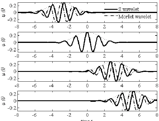
[image:42.596.185.454.418.623.2]

By analogy there is a clear similarity between equations (2.14) and (2.38); however, there are certain differences to note. First, the CWT uses the notion of scale which has an indirect relation to the frequency depending on the wavelet frequency – scale law, while the ST is defined as a function of frequency. Secondly, when generating the Morlet wavelet family the phase of the oscillatory part is continuously varied by means of the translation parameter b. In the case of the ST, the phase of the harmonic remains fixed as it can be observed in Figure 2.11. As a result, the localizations of the amplitude and phase spectra are independent from each other, property known as absolutely referenced (i.e. “fixed”) phase information (Stockwell et al., 1996).

Figure 2.11. The difference between the Swavelet and the Morlet wavelet: in the case of S -Transform the phase is absolutely referenced to the initial point.

(43)

Chapter 2 Time-frequency analysis techniques is secured through to the direct relationship with the Fourier spectrum (Ventosa et al, 2008):

 

2

( , ) i ft

f

f t ST b



dbe  d



 

 



 

(2.41)

Several windows have been proposed for the ST in order to improve its adaptability to various applications. McFadden et al. (1999) modified the Gaussian window by adding an exponential tail after the peak is attained. According to the authors, this generalized ST can accommodate any suitable function, without any restrictions on the symmetry. Stockwell (1999) generalized the S-transform by ensuring more flexibility in the choice of the dilation parameter by means of the parameter k, which can take various values i.e.

k

a

f



(2.42)

Pinnegar & Mansinha (2004) introduced a symmetrical window which incorporates an extra parameter controlling the phase modulation and connecting the S-transform with the chirplet transform.

The S-transform has been applied to a wide range of applications, from detecting damage (faults) in machineries (McFadden et al., 1999) to denoising seismic signals (Pinnegar & Eaton, 2003; Askari & Siahkoohi, 2008; Parolai, 2009).

2.6. THE EMPIRICAL MODE DECOMPOSITION

(44)

Chapter 2 Time-frequency analysis techniques instant they have zero-mean and (ii) the number of extremes is equal to / or differs by one from the number of zero-crossings. An example of the EMD performed for a simple signal is presented in Figure 2.12.

The scope of the EMD is to decompose highly non-stationary signals into simpler functions, which are characterized by a unique frequency component at each time instant (i.e. mono-component signals). This leads to a clear and straight forward characterization of the underlying frequency content distribution and evolution, which can be obtained by applying the Hilbert transform to the resulting IMFs (Huang et al, 1998).

Figure 2.12. Intrinsic mode functions (IMFs) and their Fourier transform coefficients of a signal

The decomposition of a signal f(t) into IMFs can be obtain through the following steps (summarized in Figure 2.13):

1. Set

h t

₀

   



f t

. 2. Identify the jth IMF:

a. Identify the local extremes of the time-series;

(45)

Chapter 2 Time-frequency analysis techniques c. Compute the mid-point between the envelopes and subtract it from the data:

 

₁

   

2

up lo

j _j

e t e t

m t

h t h _ t m t

 

 

(2.43)

d. Check if the IMF criteria are met; if yes

IMF t

_i

 



h t

_j

 

; otherwise repeat steps a-c until the IMF criteria are met;

3. Obtain the residual signal by extracting the IMF from the data

 

₀

 

i

 

i

r t



h

t



IMF t

(2.44)

4. Repeat the procedure until the residual becomes a monotonic function or has maximum two extreme values.

Figure 2.13. Empirical mode decomposition scheme

(46)

Chapter 2 Time-frequency analysis techniques steps 2.a.- 2.c. need to be repeated several times in order to obtain adequate IMFs. The role of this process is to avoid having two frequency components at the same instant and to obtain more symmetrical waveforms. This refining procedure is known as sifting and continues until pre-set stopping criteria like are met. Such stopping criteria can be thresholds for the amplitude of h(t) or a fixed number of siftings (Huang et al, 1998; Huang et al, 2003; Rilling et al., 2003). Caution should be exercised when choosing the stopping criteria: they have to be strict enough to ensure the components are realistically separated, but on the other hand they have to be flexible enough not to cause smoothing of the data and thus lead to unrealistic results (Huang et al, 2003).

The EMD decomposes the signal into a small number of intrinsic components compared to the FFT or the WT. The resulting IMFs are locally orthogonal to each other, however global orthogonality is not necessarily ensured, as it can be observed (Figure 2.12). From this perspective, the algorithm has been compared with an overlapping filter bank (Flandrin et al., 2004). Although mono-component, the resulting IMFs are not stationary, their frequency and amplitude varying over time. The high adaptability to the data and the intuitive, simple algorithm used for the EMD attracted the interest of researchers from different fields. On the other hand, due to the fact that it is based on an empirical algorithm rather than a mathematical formulation, any statistical processing of the results is quite challenging, limiting the use of the EMD mostly for characterization of specific records, i.e. seismic signals (i.e. Loh et al., 2001; Huang et al, 2001; Zhang et al., 2003; Spanos et al., 2007; Yinfeng et al., 2008), water waves (Dätig & Schlurmann, 2004), wind data (Huang et al., 1998), for denoising (Guo et al., 2012) or for damage detection (Xu et al., 2010).

(47)

CHAPTER 3 :

PULSE-LIKE GROUND MOTIONS

CHARACTERIZATION, EXTRACTION AND

SIMULATION

3.1. PRELIMNARY REMARKS

Pulse-like seismic ground motions are characterized by the presence of high amplitude, long period pulses, which severely influence the behaviour of a wide range of relatively flexible structures in the affected areas. Historically, pulse-like ground motion (PLGM) related research started with the 1952 Kern County (California) event, followed by the 1966 Parkfield and the 1971 San Fernando (California) earthquakes. However, more extensive research efforts were devoted after the 1994 Northridge (California), 1999 Kobe (Japan) and 1999 Izmit (Turkey), 1999 Chi Chi (Taiwan) events, which caused significant structural damage especially in the case of buildings with medium to long natural periods (Sommerville 1997, 1998, 2000, 2002; Moustafa & Takewaki, 2010; Mavroeidis & Papageorgiou, 2003, Tang & Zhang, 2011). Aiming to improve the structural behaviour in the regions likely to be subjected to such ground motions, but also for seismic risk assessment studies, there is a lot of interest currently focussing on this topic. Several themes were identified in the PLGM related research, namely (i) the identification of the physical conditions which favour their occurrence and (ii) the identification of measurable distinguishing features, based on which they can be (iii) modelled and then (iv) simulated for the purpose of seismic risk assessment.

(48)

Chapter 3 Pulse-like ground motions values and structural impact in order to identify distinct features which are commonly associated with PLGMs. Further, the physical causes presented in the literature as sources for PLGMs are summarized and the parameters employed for pulse characterization are presented. The pulse models existing in the literature are also discussed, followed by the commonly used approaches for identification and extraction of pulses from records, which include:

(i) fitting simplified, deterministic pulse models to time-domain representation of the signal (Menun & Fu, 2002; Mavroeidis & Papageorgiou, 2003; Moustafa & Takewaki, 2010; Yaghmaei-Sabegh, 2010) or to their response spectra (Tang & Zhang, 2011);

(ii) applying time-frequency signal processing techniques to the acceleration or velocity traces (Zhang et al, 2005; Baker, 2007; Xu & Agrawal, 2010; Vassiliou & Makris, 2011);

(iii) filtering the low-frequency content of the signal (Ghahari et al., 2010; Mukhopadhyay & Gupta, 2013a).

In the final section of this chapter the modelling approaches employed for PLGMs representation and/or simulation are presented.

3.2. PHENOMENOLOGICAL AND PHYSICAL

CONSIDERATIONS

(49)

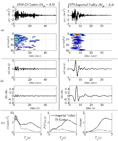
Chapter 3 Pulse-like ground motions In Figure 3.1.a, the distribution of the energy content in time and in frequency (TFD) is displayed for each accelerogram. The TFDs are obtained using the continuous wavelet transform and employing the generalized harmonic wavelets as decomposing functions, following the methodology presented in Section 2.4.6. It can be observed that both are characterized by broadband frequency content. In the case of the pulse-free accelerogram belonging to the El Centro event, the distribution of the energy in frequency is relatively uniform over the interval ~[5, 15]rad/s, while for the pulse-like Imperial Valley record most of the energy is concentrated in the low-frequency interval under ~5 rad/s. A first distinguishing aspect for PLGMs is thus the concentration of a significant amount of the total energy released during the earthquake in a narrow and very low-frequency band.

(50)

[image:50.596.123.539.111.606.2]

Chapter 3 Pulse-like ground motions when subjected to pulse-like ground motions (e.g. Alavi & Krawinkler, 2001; Tothong & Cornell, 2008; Sehhati et al, 2011).

Figure 3.1. Non-pulse ground motion versus pulse-like ground motion of similar magnitudes and peak ground accelerations, recorded at Imperial Valley, Southern California: (a) accelerograms and their corresponding frequency energy distributions; (b) velocity and displacement

time-histories; (c) 5% elastic response spectra

(51)

Chapter 3 Pulse-like ground motions has been observed that near-fault areas (i.e. located at 5-20(30) km from the seismic fault), are more likely to experience this type of ground motion as a consequence of the directivity effect or of the fling step effect. For this reason, pulse-like earthquakes are commonly referred to as near-field (fault) earthquakes, although it should be noted that not all the ground motions experienced in the proximity of seismic faults are of pulse-type (Iervolino & Cornell, 2008; Shahi & Baker, 2011).

The directivity effect is a dynamic phenomenon, caused by the tendency of the fault rupture to concentrate the wave energy along the fault. Depending on the position relatively to the fault, a specific site can experience “forward-directivity”, when the rupture propagates towards the site or “backward-directivity”, for ruptures propagating away from the site. The time-histories recorded as a consequence of forward-directivity (FD) effect have shorter duration and present large amplitude velocity pulses at the beginning of the records. The time-histories recorded in the case of backward-directivity have longer durations and small amplitudes (Sommerville, 1997; Dabaghi & Der Kiureghian, 2011).

Figure 3.2. Schematization of the forward directivity effect (planar view)

Wavelet-Based Characterization and Stochastic Modelling of Pulse-like Ground Motions on the Time-frequency Plane

City, University of London Institutional Repository

Citation

:

This is the accepted version of the paper.

This version of the publication may differ from the final published

version.

Permanent repository link:

Link to published version

:

Copyright and reuse:

City Research Online aims to make research

outputs of City, University of London available to a wider audience.

Copyright and Moral Rights remain with the author(s) and/or copyright

holders. URLs from City Research Online may be freely distributed and

linked to.