City, University of London Institutional Repository
Citation:
Kearns, James (2012). Comparing the risks of diverse methods of electricity generation using the J-value framework. (Unpublished Doctoral thesis, City University London)This is the unspecified version of the paper.
This version of the publication may differ from the final published
version.
Permanent repository link:
http://openaccess.city.ac.uk/1321/Link to published version:
Copyright and reuse: City Research Online aims to make research
outputs of City, University of London available to a wider audience.
Copyright and Moral Rights remain with the author(s) and/or copyright
holders. URLs from City Research Online may be freely distributed and
linked to.
COMPARING THE RISKS OF DIVERSE
METHODS OF ELECTRICITY
GENERATION USING THE J-VALUE
FRAMEWORK
by
JAMES KEARNS
Volume II
A thesis in two volumes
Submitted in fulfilment of the
requirements for the degree of
Doctor of Philosophy
THE CITY UNIVERSITY
School of Engineering and Mathematical Sciences
Table of Contents
Volume I
Table of Contents ... 2
List of Figures ... 6
List of Tables... 9
Acknowledgements ... 14
Declaration ... 16
Abstract ... 17
Nomenclature ... 18
Chapter 1 Introduction ... 24
1.1 Statement of Problem ... 24
1.2 Aims and Objectives ... 24
1.3 Structure ... 24
Part 1 Valuing Health and Safety ... 27
Chapter 2 Historical Context and Existing Literature ... 30
Chapter 3 Conceptual Foundations of the J-Value ... 38
3.1 The Life Quality Index ... 38
3.2 The Trade-Off between Free Time Fraction and Income ... 40
3.3 The Trade-Off between Income and Life Expectancy ... 45
3.4 Utility and Discounting in the Life Quality Index ... 48
3.5 The J-Value ... 54
Chapter 4 Fundamental Relationships between Parameters Used in Life-Expectancy Calculations ... 60
4.1 Characterising and Modelling the Survival of Populations ... 60
4.2 The Hazard Rate and the Survival Probability ... 61
4.3 The Survival Probability and Life Expectancy ... 64
4.4 Relationship to the Life Table Functions ... 66
4.5 Calculation of Life Expectancies in the J-Value Model ... 71
4.6 The Steady State Population Distribution ... 73
4.7 The Average Life Expectancy ... 75
4.8 The Effect of Discounting on Life Expectancy... 77
Chapter 5 Calculations for the Change in Life Expectancy Following a Hazard Perturbation ... 81
5.1 Modelling Changes in Life Expectancy ... 81
5.2 Exposures ... 82
5.3 Responses ... 83
5.4 Increase in Hazard Rate – Absolute and Relative Models ... 83
5.5 Increase in Cumulative Hazard Rate ... 85
5.6 Decrease in Life Expectancy ... 85
5.8 Limiting Exposure and Response Distributions ... 87
5.9 Modelling the Effects of Radiation and Pollution... 94
5.10 Accounting for those Entering and Leaving the Population during a Prolonged Exposure ... 105
5.11 The Effect of Discounting on the Hazard Rate Perturbations ... 109
Chapter 6 Fundamental Relationships for the Calculation of Work-Life Expectancy and the Work-Time Fraction ... 114
6.1 Characterising Working Time Behaviour ... 114
6.2 The Work-Time Fraction ... 114
6.3 Work-Life Expectancy ... 115
6.4 Approximations for the Work-Time Fraction ... 119
Chapter 7 The Value of Life and Life-Years ... 121
7.1 The Value of Delaying a Fatality ... 121
7.2 The Value of Temporarily Preventing a Fatality, VTPF... 123
7.3 The Value of a Discounted Life-Year, VODLY ... 124
7.4 An Alternative Model of the VODLY, the VODLYA ... 126
7.5 The Hazard Elimination Premium, HEP ... 127
Chapter 8 Measurement of the Parameters Required for J-Value Analysis and their Tolerances ... 129
8.1 Quantifying Parameters and their Uncertainty ... 129
8.2 Gross Domestic Product per Person, G ... 131
8.3 Net Discount Rate, r , Discount Rate, rd and Growth Rate, rg ... 133
8.4 Discounted Average Life Expectancy, Xd, and Other Related Actuarial Parameters ... 133
8.5 Share of Wages in the GDP, θ ... 140
8.6 Work-Life Parameters and Risk Aversion, ε ... 142
8.7 Change in Discounted Life Expectancy, δXd ... 144
8.8 Other Context-Dependent Parameters... 158
8.9 The J-Value ... 159
8.10 The VTPF, VODLY and VODLYA ... 162
Chapter 9 Sensitivity Analysis of the J-Value Framework ... 174
9.1 The Purpose of Sensitivity Analysis ... 174
9.2 The Sensitivity Coefficients of the J-Value ... 174
9.3 Sensitivity Analysis of the Life Expectancy Calculations ... 176
9.4 Sensitivity Analysis of the Risk Aversion Calculations ... 182
Chapter 10 Extending the J-Value Framework to Include Mitigation of Financial Risks ... 191
10.1 The J2 and JT-Values ... 191
10.2 The Baseline, Risk Neutral Spend on Risk Reduction ... 191
10.3 Accounting for Risk Aversion Using the ABCD Model ... 193
10.4 The Maximum Reasonable Spend and the New J-Values ... 199
Chapter 11 Example Calculations ... 206
11.1 Example Calculations for the J-Value... 206
11.3 Department of Health’s Proposal to Reduce the Number of Unnecessary
CT Scans ... 208
11.4 Department of Health’s Proposal to Reduce the Number of MRSA Infections ... 209
11.5 Example Calculations for the J2 and JT-Value: Mitigating Large Nuclear Accidents ... 210
11.6 J-Value Analysis of the Ancient VTPF ... 212
Volume II
Table of Contents ... 2List of Figures ... 6
List of Tables... 9
Part 2 Comparative Risk Analysis of Electricity Generating Systems in the United Kingdom ... 14
Chapter 12 Literature Review ... 16
Chapter 13 Overview of the Analysis ... 24
13.1 Scope of the Report ... 24
13.2 System Boundaries ... 26
13.3 Calculation of Impacts ... 28
13.4 Quality of Data ... 32
13.5 Issues with Aggregation and Presentation of Results ... 34
Chapter 14 Materials and Transportation Impacts ... 39
14.1 General Impacts in the Construction Materials Chain ... 39
14.2 Impacts Resulting from Transportation ... 41
14.3 Impacts Resulting from the Use of Steel ... 42
14.4 Impacts Resulting from the Use of Concrete ... 50
14.5 Impacts Resulting from the Use of Non-Ferrous Metals ... 52
14.6 Impacts Resulting from the Use of Glass ... 54
14.7 Impacts Resulting from the Use of Plastic ... 55
Chapter 15 The Nuclear Fuel Chain ... 75
15.1 Description of the Fuel Chain ... 75
15.2 Plant Parameters ... 77
15.3 Extraction ... 79
15.4 Preparation ... 82
15.5 Generation ... 83
15.6 Reprocessing ... 87
15.7 Waste Storage and Disposal ... 88
15.8 Materials ... 90
15.9 Transportation ... 90
15.10 Summary and Discussion ... 91
Chapter 16 Fossil Fuel Chains ... 105
16.1 Description of the Fuel Chains ... 105
16.3 Extraction ... 106
16.4 Preparation ... 108
16.5 Generation ... 109
16.6 Waste Disposal ... 110
16.7 Materials ... 111
16.8 Transportation ... 111
16.9 Summary and Discussion ... 111
Chapter 17 Wind Fuel Chains ... 124
17.1 Description of the Fuel Chains ... 124
17.2 Plant Parameters ... 124
17.3 Generation ... 125
17.4 Materials ... 126
17.5 Transportation ... 127
17.6 Summary and Discussion ... 127
Chapter 18 Comparative Analysis ... 134
18.1 Presentation of Results ... 134
18.2 Immediate Occupational Impacts ... 135
18.3 Immediate Public Impacts ... 136
18.4 Delayed Occupational Impacts ... 137
18.5 Delayed Public Impacts... 138
18.6 Impacts Resulting from Abnormal Operation ... 139
18.7 Aggregated Measures of Risk ... 140
Chapter 19 Discussion ... 155
19.1 Sensitivity Analysis ... 155
19.2 General Discussion... 159
19.3 Implications for Future Generation Scenarios ... 160
19.4 Comparisons with Other Studies ... 161
Part 3 Conclusions and Further Work ... 179
Chapter 20 Conclusions ... 179
20.1 Conclusions Regarding the J-Value Framework... 179
20.2 Conclusions Regarding the Comparative Risk Analysis ... 180
20.3 Overall Conclusions ... 183
Chapter 21 Further Work ... 185
21.1 Further Work Regarding the J-Value ... 185
21.2 Further Work Regarding the J2 and JT-Values ... 185
21.3 Further Work Regarding the Comparative Risk Analysis ... 186
Bibliography ... 191
Appendices ... 209
Appendix A. Proof that the Maximum Reasonable Spend on Human Protection is Invariant under Affine Transformations of the Utility Function ... 209
Appendix B. Proof that the Moments of the Life to Come are Equal to the Moments of the Life Already Lived in a Steady State Population ... 216
Appendix C. Description of Ferguson’s Method for Estimating the Loss of Life Expectancy Resulting from Occupational Dust Exposures ... 222
List of Figures
Volume I
Figure 1 Indifference curves of quality of life against the income constraint. ... 57
Figure 2 Discounted life expectancy versus life expectancy at r = 2.5% pa, based on ONS figures. ... 58
Figure 3 J = 1 indifference curve for income against (undiscounted) life expectancy. ... 59
Figure 4 Population distributions calculated from UK data for 2007-2009... 80
Figure 5 Exposure rate, b(x), over time, x. ... 111
Figure 6 Probability density for the mortality period, y. ... 111
Figure 7 The excess mortality probability distribution for radiation-induced cancer. ... 112
Figure 8 The excess mortality distribution for pollution-induced mortality. ... 112
Figure 9 Probability distribution of the GDP per person estimate. ... 164
Figure 10 Historical data showing how the UK GDP and population size are correlated. ... 165
Figure 11 Life expectancy, Xd(a), and average life expectancy, Xd. ... 166
Figure 12 Historical data showing the variation in the wage share of the GDP, θ, for the UK from 1955. ... 167
Figure 13 Time series data from the work time fraction, w0, the wage share of the GDP, θ, and the risk aversion, ε, for available data from 1984 to 2008. ... 168
Figure 14 Normal-quantile plot for risk aversion normality test. ... 169
Figure 15 Values of the age dependent VTPF, and the age-averaged VTPF, for discount rates 0% and 2.5%. ... 170
Figure 16 Values of the VODLY and VODLYA, for discount rates of 0% and 2.5%. ... 171
Figure 17 Result of Pearson’s chi-square test for 24 tests. ... 186
Figure 18 Difference between the linear approximation and the exact calculation of the change in life expectancy, as a function of the hazard rate. ... 187
Figure 19 Rectangular distributions for gw(t), pw(t) and pw(t)gw(t) ... 188
Figure 21Response of the reluctance to invest (R120A) with increasing risk aversion
(ε), for different normalised costs of the safety system (-0.1 < b < 0.6). ... 201
Figure 22 The derivative of the reluctance to invest when ε = 0.5 and c = 0.9, illustrating the two roots of the objective function g(ε, b) = 0. ... 202
Figure 23 The derivative of the reluctance to invest when ε = 0.9 and c = 0.999, illustrating the two roots of the objective function g(ε, b) = 0. ... 203
Figure 24 The derivative of the reluctance to invest when ε = 1.5 and c = 0.9, illustrating the single root of the objective function g(ε, b) = 0. ... 204
Figure 25 The derivative of the reluctance to invest when ε = 1.5 and c = 0.999, illustrating the single root of the objective function g(ε, b) = 0. ... 205
Figure 26 Dose received by individual of age a who is undergoing scans at future age t. ... 215
Figure 27 The response of the additional risk faced by an individual of current age a at future age t, following an exposure type given in Figure 26... 216
Volume II
Figure 28 Fuel chain (from top to bottom) and construction materials chain (from left to right) used in the analysis. Arrows indicate transportation processes. ... 37Figure 29 Diagram of current and new build risk and output levels. Current impacts = R1/O1, future impacts = R2/O2 and incremental impacts = ΔR/ΔO. ... 38
Figure 30 Incremental immediate occupational risks for each technology. ... 144
Figure 31 Incremental immediate public risks for each technology. ... 145
Figure 32 Incremental delayed occupational risks for each technology. ... 146
Figure 33 Incremental delayed public risks for each technology. ... 147
Figure 34 All incremental immediate risk for each technology. ... 148
Figure 35 All incremental delayed risk for each technology. ... 149
Figure 36 All incremental occupational risk for each technology. ... 150
Figure 37 All incremental public risk for each technology... 151
Figure 38 All incremental normal operation risk for each technology. ... 152
Figure 39 All incremental abnormal operation risk for each technology. ... 153
Figure 40 Total incremental risk for each technology. ... 154
Figure 42 Public and occupational risk proportions of total impacts... 166
Figure 43 Immediate and delayed risk proportions of total impacts. ... 167
Figure 44 Normal and abnormal operation risk proportions of total impacts. ... 168
Figure 45 Comparison of immediate occupational fatality risks. ... 169
Figure 46 Comparison of delayed occupational fatality risks. ... 170
Figure 47 Comparison of immediate public fatality risks. ... 171
Figure 48 Comparison of delayed public fatality risks. Note the logarithmic scale. ... 172
Figure 49 Comparison of total risk. Note the logarithmic scale. ... 173
Figure 50 Relationship between power utility risk aversion, εp, and the Atkinson risk aversion, εA. ... 215
Figure 51 Exponential trend lines used in the extrapolation of the collective loss of life expectancy from CWP and silicosis. ... 225
List of Tables
Volume I
Table 1 Summary of literature on valuation of mortality risks. ... 36
Table 2 Hazard rate perturbations for limiting exposure and response distributions, assumed to be uniform over the specified period... 113
Table 3 Values of the compensating factor and dose-risk coefficient for different populations, using latest data. ... 113
Table 4 Data for the normal-quantile plot to test the risk aversion for normality. .. 172
Table 5 Results of the normal-quantile plot. ... 172
Table 6 Values of parameters ... 173
Table 7 Life expectancy under different population distributions. ... 190
Table 8 Work-life expectancy under different population and working time distributions. ... 190
Table 9 Work-time fraction under different population and working time distributions. ... 190
Table 10 Risk aversion under different population and working time distributions. The wage share θ is taken as 0.563, which was calculated for 2008 data. ... 190
Table 11 Deaths avoided and life-years gained for the four exposure limits from HSE’s assessment of methods to reduce occupational exposures to respirable crystalline silica. ... 217
Table 12 Cost of scheme and J-values using Table 11 data. ... 217
Table 13 Data for DH’s proposal to implement COMARE’s recommendations. ... 217
Table 14 Data for DH’s proposal to reduce the number of MRSA deaths. ... 217
Table 15 Loss of life expectancy to public and workers following a notional large nuclear accident. ... 218
Volume II
Table 16 Summary of literature on UK comparative risk analyses. ... 23Table 17 HGV statistics, from [62], [63] and [64]. ... 59
Table 18 Train freight and passenger statistics, from [65] and [153]. ... 59
Table 20 Summary of transport exposure rates... 59
Table 21 UK production of stone, from [25]. ... 60
Table 22 UK production of minerals, from [25]. ... 60
Table 23 UK production of selected manufactured materials, from [25]. ... 61
Table 24 Quantities of recycling and waste production, from [58] and [59]. T ... 61
Table 25 HSE fatality statistics for extractive industries classed under “other mining and quarrying”. ... 62
Table 26 HSE fatality statistics for extractive industries classed under “mining of coal and lignite; extraction of peat”. ... 62
Table 27 UK offshore fatalities, 2006 – 2010, see Table 86 for further details. ... 63
Table 28 HSE fatality statistics under classification “basic metals” in manufacturing section. ... 63
Table 29 HSE fatality statistics under classification “non-metallic mineral products” in manufacturing section. ... 63
Table 30 HSE fatality statistics attributed to recycling of metals and non-metals, and for waste the wholesale and treatment of waste. ... 64
Table 31 PM2.5 emissions for manufacturing industries, and collective exposures, from [56], [57] and [158]. ... 65
Table 32 PM2.5 emissions for extractive and disposal industries, and collective exposures, from [56] and [57]. ... 65
Table 33 PM2.5 emissions from transportation processes, from [56] and [57]. ... 66
Table 34 Summary of impacts associated with extraction processes, in terms of years of lost life expectancy/Mt ... 67
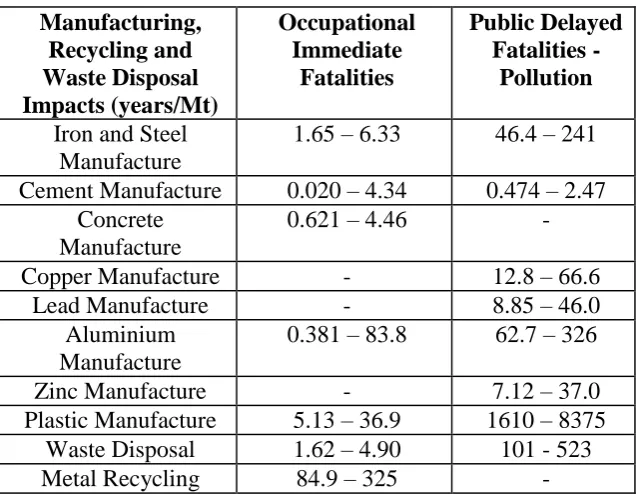
Table 35 Summary of manufacturing, waste disposal and recycling impacts. ... 67
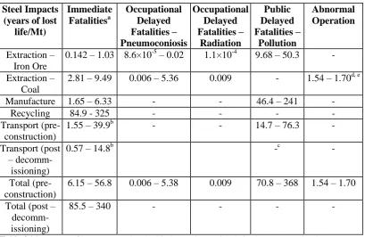
Table 36 Summary of impacts associated with the steel material chain. ... 68
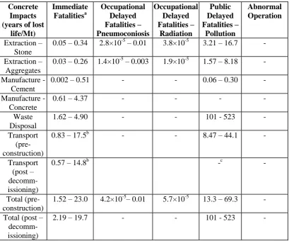
Table 37 Summary of impacts associated with the concrete material chain. ... 69
Table 38 Summary of impacts associated with the copper material chain. ... 70
Table 39 Summary of impacts associated with the lead/zinc material chain. ... 71
Table 40 Summary of impacts associated with the aluminium material chain. ... 72
Table 41 Summary of impacts associated with the glass material chain. ... 73
Table 42 Summary of impacts associated with the plastic material chain. ... 74
Table 44 Lifetimes, capacities and capacity factors and remaining output of UK
nuclear facilities from 2010 to 2070. ... 95
Table 45 Assumptions used for new nuclear plants. ... 96
Table 46 Areva employment figures, 2004 – 2009. From [3], [4], [5], [6]. ... 96
Table 47 Areva fatality figures, 2004 – 2009. From [3], [4], [5], [6]. ... 96
Table 48 Areva global market share and inferred global average fatalities ... 96
Table 49 Uranium mines output, safety data and exposure rates. ... 97
Table 50 Exposure rates at the preparation stage. ... 97
Table 51 Predicted collective doses arising from emissions of radionuclides for the EPR and AP1000 new PWR reactors. ... 97
Table 52 Employment and doses to the workforce. ... 98
Table 53 Public collective doses. ... 100
Table 54 AP1000 Release frequencies and resulting collective doses. See [201]. .. 101
Table 55 Data for reference large nuclear accident. ... 101
Table 56 Material requirements for new build. ... 102
Table 57 Current hazard elimination premiums for various impacts arising at different fuel chain stages. ... 103
Table 58 Incremental hazard elimination premiums for various impacts arising at different fuel chain stages. ... 104
Table 59 Operation and decommissioning lifetimes of UK coal facilities, including assumed lifetimes for reference facilities, and capacities, capacity factors and remaining output from 2010 to 2070. ... 114
Table 60 Operation and decommissioning lifetimes of UK gas CCGT facilities, including assumed lifetimes for reference facilities, and capacities, capacity factors and remaining output from 2010 to 2070. ... 116
Table 61 Assumed construction, operation and decommissioning lifetimes of new CCGT and coal plants, and assumed capacity and capacity factors. ... 117
Table 62 Occupational collective doses. ... 117
Table 63 Public collective doses. ... 117
Table 64 Particulate matter emissions from E.On UK coal plants. New Build plant is assumed to operate at full load. ... 118
Table 65 Particulate matter emissions from E.On UK gas plants. ... 118
Table 67 Material requirements for new gas build, and the safety data for material fabrication. ... 119 Table 68 Current coal hazard elimination premiums for various impacts arising at different fuel chain stages. ... 120 Table 69 Incremental coal hazard elimination premiums for various impacts arising at different fuel chain stages. ... 121 Table 70 Current gas hazard elimination premiums for various impacts arising at different fuel chain stages. ... 122
Table 71 Incremental gas hazard elimination premiums for various impacts arising at different fuel chain stages. ... 123 Table 72 Construction, operation and decommissioning lifetimes, and capacity factors for current wind plants. ... 129 Table 73 Construction, operation and decommissioning lifetimes, and assumed capacity factors for new build wind plants ... 129 Table 74 Material requirements for onshore and offshore wind turbines. ... 129 Table 75 Current onshore wind hazard elimination premiums for various impacts arising at different fuel chain stages. ... 130 Table 76 Incremental onshore wind hazard elimination premiums for various impacts arising at different fuel chain stages. ... 131 Table 77 Current offshore wind hazard elimination premiums for various impacts arising at different fuel chain stages. ... 132 Table 78 Incremental offshore wind hazard elimination premiums for various impacts arising at different fuel chain stages. ... 133 Table 79 Summary of current impacts from each technology. ... 142 Table 80 Summary of incremental impacts from each technology... 142 Table 81 Summary of current of risks from each technology, aggregated by impact
categories. Impacts are due to normal operation. Impacts from abnormal operation are shown in brackets. ... 143
Table 84 Collective loss of life expectancy from CWP and silicosis. ... 224
Table 85 Average age of death for CWP and silicosis deaths. ... 224
Table 86 UK Energy fatalities between December 2005 – November 2010. Major data sources: [1], [40], [103], [104], [131]. ... 229
Table 87 UK generation of electricity by the assessed technologies. Data from [49]. ... 230
Table 88 UK production of natural gas [48]. ... 230
Table 89 UK production of oil [46]. ... 230
Part 2 Comparative Risk Analysis of Electricity Generating
Systems in the United Kingdom
The intention of the second part of this thesis is to evaluate and compare risks to human life posed by electricity generating systems within the UK. This is done by using the J-value framework to evaluate the loss of life expectancy from a variety of sources of risk, as described in part 1. In addition to this, financial risks resulting from large accidents causing environmental damage will also be evaluated using the J2-value approach described in chapter 10, although the main focus of the work will be regarding human risks. The chosen technologies for analysis are nuclear, coal, natural gas, onshore wind and offshore wind, which together currently generate over 90% of the UK’s electricity, and will likely continue to do so in the near future, for example, see DECC (2011d) [51]. A complete fuel-chain approach has been taken, in which impacts involved with all stages from extraction to waste disposal are
considered.
This is the first research to evaluate risks from such systems using the J-value method to monetise the risks. Monetisation is achieved by calculating the theoretical cost that would be required in order to eliminate all risks presented by electricity generating systems that would give J = 1. This quantity is the “hazard elimination premium” (HEP), which was introduced in chapter 7, where the usefulness of this
quantity in risk comparison was discussed. This cost can be interpreted as the additional burden on human health resulting from the generation of electricity. This cost is then the “external cost of risk”, a term more commonly used in the literature,
see, for example ExternE (1995) [77]. For financial risks, the maximum reasonable cost of eliminating that risk can be calculated directly. This is simply the quantity,
δZR, of equation (10.7). Other new contributions made in this thesis include the use
Chapter 12 Literature Review
The practice of comparing risks quantitatively is a relatively recent phenomenon. It arose in the mid-seventies in response to, and as a means to address public concern
with complex technologies that were imposing unfamiliar hazards on both humans and the environment. Research into the psychology of risk had demonstrated that
perceptions of risk by non-experts were frequently at odds with the true magnitude of the risk. In particular, risks that were familiar tended to be underestimated, whilst unfamiliar risks were usually overestimated, see Lichtenstein et al (1978) [130]. Comparative risk analysis was therefore put forward as a tool that could aid in informing the public of the nature of the new hazards posed by an expanding industrial sector, the rationale being that such comparisons give risks a context and provide a frame of reference that is more intuitive and more meaningful to the user than absolute values considered in isolation.
The literature on comparative risk analyses can be divided into two categories, as is done by Covello (1991) [43]. These are: comparisons of diverse sources of risk, and comparisons of similar sources of risk. The former typically uses measures such as the annual death rate, or collective loss of life expectancy as a common unit of risk, and compares a wide variety of hazardous activities and causes of death. One of the earliest major studies of this kind was by Cohen and Lee (1979) [37], who produced a “Risk Catalogue”, which used loss of life expectancy to compare a somewhat
eclectic collection of risks. Some of the greatest risks calculated in this study were of remaining unmarried, smoking, heart disease and being a coal miner, whilst the least hazardous activities were from the operation of nuclear power plants. Another early
major study of this type was by Crouch and Wilson (1982) [46], who calculated the required time for which exposure to the risk would increase the probability of death by one in one million. The activities which required the least amount of time according to this measure were: fire fighting, coal mining, railroad employment and police duty.
implement or prioritise. Whilst the first type of study is useful for providing risks in context, and therefore aids the judgement of the acceptability of any new risk, the second type of study informs the public and decision makers about the likely prospects of different courses of action. The analyses of comparative risks from energy and electricity production technologies are of this second type. One of the earliest studies of this type was by Lave and Freeburg (1973) [128], which compared health effects of electricity generation by coal, oil and nuclear fuel. The Atomic Energy Commission (1974) [14] compared fossil fuels with nuclear and
hydroelectric power. Comar and Sagan (1976) [38] also published studies that compared the risks from nuclear power to fossil fuels, whilst Caputo (1977) [28] published one of the earliest studies comparing non-conventional electricity generating technologies to conventional fossil fuel technologies. This study compared orbital solar power plants that transmit solar power to earth by microwave with ground based solar plants and conventional nuclear and fossil plants. The most widely known comparative risk assessment of energy technologies of this period was the study by Inhaber (1978a) [109] on behalf of the Atomic Energy Control Board of Canada, summaries of which were also published in various journals and magazines see Inhaber (1978b) [110], and (1979) [111]. This report used “risk accounting” – a method of evaluating all sources of risk at each stage of the energy production chain (what would now be known as life-cycle analysis) to compare the total risk of eleven different energy technologies, including coal, oil, natural gas, nuclear, wind, hydroelectricity, ocean thermal, methanol and three types of solar technologies. The study was the most systematic and rigorous of all the risk comparison literature of the period. Nevertheless, the conclusions of the report – that non-conventional energy technologies were not inherently low risk – provoked furious criticism (see, e.g. Holdren (1979) [97]). The final revision of the report, as well as most of the
critical comments, were published in a subsequent book, see Inhaber (1982) [112].
pneumoconiosis deaths, and cancer deaths, all of which were evaluated per unit of electricity generated. The plants studied were assumed to have a capacity of one gigawatt, and operated at 75% of this capacity. The authors of this report emphasised the importance of studying whole systems, and partitioned their data into the following fuel chain stages:
Fuel extraction, processing and fabrication
Power plant operation
The authors also reviewed some selected major accident risks, which were compared with some major risks from non-fossil or nuclear energy systems in an attempt to provide some context.
This was followed a similar report published by Ferguson(1989)[83], on behalf of the Newcastle Energy Centre, which also studied coil, oil and nuclear technologies.
The nuclear power plant was assumed to be an advanced gas-cooled reactor (AGR). The risk measures used were occupational and public accidents and disease,
evaluated, again, per unit of electricity generated. The fuel chain stages were partitioned more finely than in the Cohen and Pritchard study, with the following stages being analysed:
Fuel extraction
Preparation and transport
Electricity generation
The author of the study warned that the results of the study must be considered in accompaniment with some caveats, which were of the uncertain nature of the estimated risks from pollution and radiation.
analyses, and identified many potential pitfalls present in both producing and interpreting the results of such analyses, as well as issues involved with conveying results to a wider audience. Pochin (1977) [162] also published a short paper comparing risks from coal, oil, nuclear, natural gas and hydroelectricity, using figures largely based on previous research. Fremlin (1987) [85] gave an excellent account of the issues of risk involved in power production, comparing coal, oil, natural gas, nuclear, hydroelectricity, wave and wind energy. Fremlin also included an estimate of the risks from a mediaeval water mill for comparison, and
interestingly, also includes an estimate of the risk from energy conservation, noting that improved insulation will cause greater exposures to pollution and radiation.
Increasing concerns about the environment and energy security brought the need for renewable technologies more sharply into focus. In 1989 Fritzsche produced an analysis of risks from a series of electricity technologies thought to be generally applicable to Europe [86]. The various technologies were split into three groups. The first group was fossil fuels, and included coal, oil, natural gas and wood. The second group was renewable energy systems, which included solar technologies, wind and hydroelectric. The third group was nuclear technologies. Risks were delineated according to whether they were occupational risks or public risks, and whether they were acute risks or delayed risks. Severe accidents were also treated separately. Risks were presented in terms of fatalities per GWa over all stages of the fuel chain. The conclusions were that the highest risks were from severe accidents of coal, oil, gas and hydroelectric, and from public delayed risks resulting from coal and oil. Renewables generally presented medium to low risks, whilst nuclear technologies presented low risks.
Ball et al (1994) [15] published the first in-depth analysis of the risks of proposed renewable energy technologies in the UK, and compared them with nuclear and
which are estimated per unit of electricity generated. The study also analysed whole fuel chains, and the data was delineated according to the following fuel chain stages:
Fuel Extraction
Fuel Preparation/Reprocessing
Materials/Component Fabrication
Plant Construction
Power Plant Operation
Transport
Decommissioning
Waste Disposal
This study also separately analysed the health impacts from pollution and major accidents, emphasising the large uncertainties inherent in the process. The authors note that defining system boundaries is essential if the analysis is to be consistent, and if the comparisons are to be meaningful. It is for this reason that risks from acquiring construction materials were included in the fuel chain, as these are major sources of risk for renewable technologies. The authors also note, however, that truncating the analysis at some point is necessary, as the system is in practice limitless. For example, the risks of acquiring materials used to construct the mine used to acquire the materials used in constructing the power plant is part of the
energy system, although most people would judge this risk as being sufficiently far removed from the energy generating process that it can be neglected. Such a truncation would always be arbitrary, and its suitability is dependent upon the judgement of the authors. In this report, a risk level of less than 0.1 fatalities or serious health detriments per gigawatt-year (GWa) is used as a guide of where risks become less significant.
systems. These damages are known as “external costs”, because their impact is
usually not reflected in the price of the energy. The project has been very rigorous and systematic in the damages it has analysed and evaluated. The initial publications compared the marginal impacts (impacts caused by building an extra power plant) of coal, lignite, oil, gas, nuclear, wind and hydroelectric energy systems, with a particular focus on the impacts in the UK and Germany. The fuel chain stages used in the project are much the same as listed above, but also include transmission of electricity to a grid (although this impact is very small). However, there was not a
single standard fuel chain used for all energy technologies, with each technology being assessed on a fuel chain that was judged to be most relevant to that particular technology. This approach means comparisons of energy technologies at stages of the fuel chain are not used. Instead, comparisons are between risk measures, such as occupational health and disease, evaluated over the whole fuel chain. For human health risks, the impacts assessed include occupational and public fatalities, injuries and diseases. Other costs assessed include amenity impacts (e.g. visual intrusion) and ecological impacts (e.g. earth movements, acid emissions and greenhouse gas emissions). Each impact is evaluated in terms of monetary cost per unit of electricity generation. Contingent Valuation methods were used for valuing mortality and morbidity reductions. The project uses a Value of Temporarily Preventing a Fatality of €2.6M. Since the initial publications in 1995, the ExternE project has expanded its
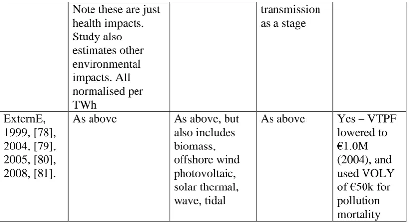
scope, including assessments of impacts in other European countries, including the new EU countries in Central and Eastern Europe. Emerging energy technologies have also been analysed, see ExternE (1999) [78], (2004) [79], (2005) [80] and (2008a) [81]. The later publications also assessed other impacts, and improved some aspects of the methodology, such as changing the valuation of air pollution impacts from number of premature fatalities to years of life lost, and including the effects
from chronic exposure to pollution, rather than just acute effects, as had been the case in earlier publications. New methods of valuing impacts were also considered,
such as inferring the external cost of eco-system damages from political negotiations.
Study Risk Measures Fuel Chains Considered Fuel Chain Stages Assessed Monetary Evaluation? Cohen and Pritchard, 1980, [35] Accidental deaths, accidental injuries, pneumoconiosis deaths, cancer deaths. All normalised per GWa Coal, oil, nuclear - Fuel extraction, processing and fabrication - Power plant operation No Ferguson, 1981, [82] Occupational accidents, occupational disease, public accidents, public disease. All normalised per GWa Coal, oil, nuclear AGR - Fuel extraction - Preparation and transport - Electricity Generation No Fritzsche, 1989, [86] Acute occupational and public fatalities, delayed occupational and public fatalities. Fatalities from severe accidents. All normalised per GWa
Coal, oil, natural gas, wood, solar – thermal, solar photovoltaic, wind, hydroelectric, nuclear LWR, nuclear HTR, nuclear FBR, nuclear fusion
Not specified No
Ball et al, 1994, [15] Acute occupational fatalities, chronic occupational disease, public delayed fatalities. All normalised per GWa
Tidal, onshore wind, offshore wind, nuclear PWR, coal, oil, gas - Fuel extraction - Preparation/ reprocessing - Materials/ component fabrication - Plant construction - Power plant operation - Transport - Decommiss-ioning - Waste Disposal No ExternE, 1995, [77] Public health, occupational health – diseases, occupational health – accidents.
Coal, lignite, oil, gas, nuclear PWR, onshore wind,
hydroelectricity
No standard fuel chain, but similar to above. Also includes electricity
Note these are just health impacts. Study also estimates other environmental impacts. All normalised per TWh
transmission as a stage
ExternE, 1999, [78], 2004, [79], 2005, [80], 2008, [81].
As above As above, but also includes biomass, offshore wind photovoltaic, solar thermal, wave, tidal
[image:24.595.114.528.70.296.2]Chapter 13 Overview of the Analysis
13.1 Scope of the Report
As discussed in the introduction to part two, risks will be evaluated for five different technologies: nuclear, coal, gas, onshore wind and offshore wind. These five technologies together account for over 90% of all electricity generated in the UK as of 2009, see DECC (2011d) [51], (gas – 43%, coal – 27%, nuclear – 19%, onshore wind – 2%, offshore wind 0.5%). These technologies are chosen as they are assumed to be representative of the UK electricity mix, both now, and in the future. The risks are assessed over a time period of 60 years, from 2010 to 2070. It is assumed that other current technologies, such as oil and hydroelectricity, emerging technologies, such as solar, tidal and biomass, and those still in development, such as nuclear fusion, will not contribute significantly to the generation of electricity within the UK
over this time period.
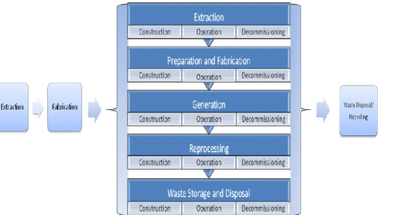
The impacts considered are human mortality risks presented over the whole of the fuel chain, as it is now recognised that any planning of electricity generation should, where possible, account for all health damages, as indirect impacts can often be a major contributor to the full social cost of the electricity supply, see e.g. IAEA (1999) [107]. In addition, financial risks associated with major accidents have also been assessed. The following fuel chain has been used where appropriate to the source of generation:
Extraction
Preparation and fabrication
Generation
Reprocessing
Waste Disposal
This fuel chain accounts for the primary fuel used in the generation of electricity. Each of these processes may be divided into three further sub-processes: construction, operation and decommissioning, although not all these stages will require assessment in every case. It is also necessary to define a separate chain that accounts for the materials used in construction of the associated facilities. This materials chain is similar to that shown above, except that there is no generation or reprocessing stage. Furthermore, not all construction materials will be eventually disposed of, as materials such as steel will be recycled. The full fuel/material chains
are shown in Figure 28.
The mortality risks are separated into occupational and public risks, and immediate and delayed fatality risks, with the latter being due to exposures from radiation, pollution (arising from emissions of particulate matter) and dust (which may cause pneumoconioses). Risks are also categorised as due to normal or abnormal operation, the latter referring to major accidents, where societal concerns may be particularly acute.
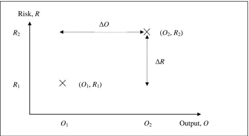
The dependence of the impacts upon the scale of growth of each technology over the period 2010 to 2070 has also been assessed. This allows impacts to be assessed on three scales: current risks, future risks and incremental risks. Current risks describe the present value of the impacts arising from the existing stock of power plants currently generating electricity over the assessed period, including all decommissioning that may take place. Future risks are those arising from both the current stock of power plants and the new build plants, where a given scale of construction can be specified. Future risks are therefore always greater than the current risks. The impacts of both current and future risks are normalised against the
amount of electricity generated over this period. For example, if the present value of all risks arising from the current stock is R1, and the amount of electricity generated
is O1, then current impacts are R1/O1. If the future risks are R2 = R1 + ΔR, where ΔR
calculated. Here, consideration will be given to current and incremental risks. The incremental risks will also form the main focus of the comparative analysis and the conclusions.
There are a number of important impacts which lie outside the scope of this report. Of these, the major impacts are: morbidity risks, such as injuries and non-fatal diseases; impacts associated with greenhouse gases and global warming; and security risks, such as those presented by terrorism.
13.2 System Boundaries
In order that meaningful comparisons can be made, it is necessary to define in a clear and consistent manner, exactly what should be included and excluded from such an analysis – i.e. what exactly constitutes a “system”. The systems under examination in this report – those of electricity generation, are by their nature very complex, both affecting and being affected by a large number of factors. This means there are no distinct boundaries by which to delineate the system, and consequently, any such definition of system boundaries must be arbitrary. This arbitrariness makes it essential that the boundaries are clearly specified, and that a high level of
consistency is maintained throughout the analysis. These boundaries are:
The time boundary:
- The majority of impacts considered occur between 2010 and 2070. - The only exception is public radiation does from nuclear plants, where
the available data used cumulative doses truncated after 500 years.
The space boundary:
- Only transportation of materials within the UK is assessed.
- Immediate public fatalities (the majority of which arise from transportation accidents) are assessed for the UK population only. - Delayed public fatalities arising from pollution are assessed for the
- Delayed public fatalities resulting from radiation are assessed over three regions: UK, Europe and the world. These regions are used to assess sensitivities as is described in section 13.4.
- Occupational impacts are assessed at the location of impact.
The resource boundary:
- All stages that involve the generating fuel, from extraction to disposal, including transportation, are assessed. Risks presented over the lifetime of the facility, from construction to decommissioning, provided they occur within the time boundary, are included.
- Impacts involved in the construction materials chain, from extraction of the raw materials, to waste disposal or recycling, and again including transportation, are included.
- Impacts outside these two chains (e.g. construction of the facility at which the material is fabricated) are excluded.
In addition to these boundaries, it is also necessary to add some caveats. It was assumed that present technologies will be used in the future. Clearly, technological change can lead to improvements in efficiencies and availabilities. Such changes would however, be impossible to predict. Assuming a constant technology for each type of electricity generation therefore is the best means of comparison.
Similarly, it is also assumed that risks per unit of electricity generated remain
constant over the timeframe of the study. This assumption is also unrealistic as most industries have experienced a trend of improving safety levels, which is likely to remain the case in the future. Predicting such changes would be impossible, and so this has not been attempted for any technology. As far as is possible, risks have been estimated from data for the most recent five-years, from 2006 to 2010.
It has also been assumed that each technology is supplying baseload energy. This means they produce electricity continuously in order to meet some or all of the UK’s
Another caveat is that all life expectancy calculations are determined from UK statistics. Clearly, a more realistic calculation would use statistics appropriate to the region concerned. However, this assumption will give conservative results, in that they overestimate the effects, rather than underestimate them. The largest overestimation will be for nuclear power, in which some uranium mining statistics were based on Namibian data, where the life expectancy is lower than in the UK. Also, if the world region was used for the collective dose estimation, then mortality statistics for the global population should be used, which would result in lower
impacts than are calculated here. Pollution impacts would not be affected greatly, as European mortality statistics are generally similar to the UK.
13.3 Calculation of Impacts
To compare the impacts from different electricity generation methods, it is necessary to use the Hazard Elimination Premium, or HEP, which is a metric developed in chapter seven. It was discussed that this metric is important for risk comparisons as it provides a valuation of the benefit obtained from eliminating the risk posed by each system. The first stage of determining the impacts is to calculate the loss of life expectancy posed by a risk. This is done by assuming that all sources of risk
contribute an additional burden upon the average mortality rates currently experienced by the population, as are given in the national interim life tables, see ONS (2009a) [145]. For sources of risk that are to be added to the system over the time period, this will be the case. However, for existing sources of risk this is slightly unrealistic, as the national mortality rates already include any fatalities that occurred in the fuel chain (within the UK). This means that the true impact would need to be estimated by comparing the current mortality rates with those that would exist if the fuel chain impacts were deleted from the national statistics. This approach has not been pursued here, which can be justified because such impacts represent a very small proportion of the national mortality rates, and so can be treated as if they were independent of them.
resulting from falls or vehicle accidents where death occurs almost immediately, or delayed fatalities, which arise from exposures to pollution and radiation, and which result in latent effects so that death does not occur until some years later. To calculate the effects of immediate fatalities, it is necessary to estimate the annual exposure rate, b (which is assumed constant over time), which is simply the average annual number of deaths D, divided by the average number of people exposed to the risk. Where possible, these averages will be performed over the most recent five years. This period is judged to be long enough to capture any natural variation in the
fatality rates, but also short enough so as to exclude data that may not be relevant to the current situation. The five year period is also favoured by the ExternE series, see ExternE (1995) [77].
For delayed fatalities, knowledge is required of the radiation doses to workers and the emissions of radiation and particulate matter (specifically, PM2.5) into the environment, which then cause public health effects. Once these are ascertained, the increase in hazard rate and the loss of life expectancy can be readily determined using the methods described in section 5.9. There are also impacts due to occupational exposures to dust from coal mining and quarrying. However, the life expectancy from these impacts is calculated from national mortality statistics, rather than through estimation of the exposure rate and the consequent probability of death. The current mortality statistics from these illnesses arise from exposures that occurred a few decades ago. In order to estimate the effects of current exposures, the present loss of life expectancy is extrapolated forward towards a point in time where the mean age of death of coal worker’s pneumoconiosis sufferers is equal to mean
age of the present workforce, which will be about 40 years from now. This method, was originally used by Ferguson [83], and is described in more detail in Appendix C.
One result that is useful for assessing the public impacts of radiation and pollution is
that the change in life expectancy is directly proportional to the exposure rate, b, i.e. that:
b
X
as can be seen from equation (8.28). The quantity δX is the individual loss of life expectancy. In the J-value framework, this quantity is then multiplied by the average number of exposed individuals, N. The product NδX may then be viewed as the collective loss of life expectancy δXcoll. This can be expressed as:
coll
coll
b
X
X
N
(13.2)where bcoll is the collective hazard rate. This formulation is useful for assessing
public exposures, where data is frequently presented in terms of the collective dose received. In such cases, the collective impact can be assessed without needing to estimate N, which simplifies the estimation procedure. However, as collective doses are commonly in excess of 100 mSv, care must be used to avoid inadvertently applying the DDREF factor, see equation (5.46). This can be avoided by dividing the collective dose by a factor of, say 1,000 or 10,000 so that the dose is below the 100 mSv threshold, calculating the loss of life expectancy, and multiplying back by that same factor. The collective loss of life expectancy can then be monetised to give the HEP. As described in chapter 7, this is the maximum reasonable cost of eliminating all risk posed by the source, such that J = 1, so that, from equation (3.61):
d d X r N N X r e X GN V V d d 1 1 ˆ (13.3)where the values of the parameters are given by Table 6.
In order to provide calculations that are normalised against the unit of energy generated, a slightly different approach may be taken. As will be discussed later, the
possible to define an additional hazard rate per gigawatt-year (GWa). If the average
electrical output of the system over the period when the D deaths occurred is O ,
then the new additional exposure rate, b*, for immediate fatalities, is:
O D
b* (13.4)
Using this exposure rate allows an additional hazard rate, δh*, and loss of life expectancy per GWa, δX*, to be calculated. If the system will give an output of O
gigawatt-years over the period under assessment, then the collective change in life
expectancy is O δX*, and the HEP is:
d d X r N X r e X GO V d d 1 1 * * (13.5)As the per person and the per gigawatt-year HEP’s are approximately independent of either the number of exposed people or the output generated, then the two measures will be approximately equal. This has the great benefit of not needing to estimate the number of people exposed to a risk, which is usually one of the most difficult parameters to assess.
Thus the usual method of calculating individual impacts scaled up by the average
number of affected individuals is broadly equivalent with the method of calculating impacts per unit electricity generation, and scaling up by the amount of electricity
generated.
The HEP per unit of electricity generated is then:
1ˆ* *
X G O VN
(13.6)
accidents, data is sparser, and so a probabilistic safety analysis has been used to determine the frequency and cost of large nuclear accidents. This data can then be used to estimate the maximum reasonable cost of eliminating the possibility of large nuclear accident over the lifetime of each power plant. This value is then the HEP for environmental risks to assets.
13.4 Quality of Data
While much of the data used in this research is reliable and known with some certainty, there still remains much data that is either not available or is by its nature highly uncertain. Such uncertainty is accounted for by presenting a range of results. Where possible, the high and low values of the range are determined from 95% confidence limits. When using fatal accident statistics, the 95% limits are calculated using Poisson statistics for cases where fatalities are rare, whereas Gaussian statistics were used for cases where accidents are frequent. In some cases, 95% confidence limits are given in the raw data. When this is not the case, high and low values are taken based on available data, and judgement is used over whether the figures are credible estimates of risk. In addition, when performing the HEP calculations, the high and low values of the input parameters, as shown in Table 6 are used for the
respective high and low estimates. Aggregation is performed by taking an appropriately weighted sum of corresponding high or low values. As discussed by Ferguson(1989) [83], the resulting sum will necessarily have a higher confidence level than its parts. A more precise root-mean-square summation could be used, but doing so would not reflect the approximate nature of some of the estimates.
could be extrapolated linearly to low doses. It was also assumed that there was no threshold at which the effect of low level doses ceases to have an effect. Thus, the conventional assumption is that any impinging ionising particle will increase the risk of premature death. This poses issues when considering collective dose, whereby the effects of routine discharges of radionuclides into the atmosphere which become globally circulated can be calculated to have a considerable effect over millions of years, due to billions of individuals receiving extremely low doses. Any such figure would be extremely speculative and should be used with caution. Indeed, the
International Commission on Radiological Protection (ICRP) has recently recommended against the use of collective dose in this way, see ICRP (2007) [113]. However, not withstanding this, and the likely pessimistic nature of the conclusions that will be reached by its use without qualification, collective dose has been used in this study as there is no established alternative such as an agreed “threshold dose”.
However, in order to estimate the likely effect of using collective dose in this way, a range of alternative assumptions on how it might be used have been considered.
In this thesis, public collective doses are determined for three populations: the UK, Europe and the world, which serve as a form of sensitivity analysis providing a range of estimates which entail differing levels of conservatism. The sensitivity of the collective dose impacts to the use of “cut-off” levels is also assessed see e.g. Jones et
al (2004) [120]. This involves neglecting all doses to individuals that are below some specified level (the “cut-off” level). For example, Jackson et al (2004) [114]
proposed a cut-off dose of 0.01 μSv/a, which results in an individual fatality risk of three orders of magnitude below levels deemed tolerable by the Health and Safety Executive (1992) [98]. Such issues also apply to other delayed impacts due to pollution and dust. It is extremely difficult to assess impacts at low doses, and for
many toxins (but not radiation unless a hypothetical cut-off is introduced), a “no observed adverse effects level” is sometimes used, taken to be a threshold below
which exposures are safe. However, in order to give better comparability with nuclear radiation, we have not applied such cut-off levels in this study.
human mortality has not been adequately studied, and so no attempt at quantification has been made here. However, these toxins can become widely circulated, and so the true impact may be substantial.
In order to assess the reliability and robustness of the results, a number of sensitivity studies have been performed, of which many have already been mentioned. These include assessing the effect of calculating radiological impacts over three different regions – the UK, Europe and the world, as well as the effect of introducing cut-off
doses. Another issue assessed for sensitivity are the coal mining statistics. This is because UK production of coal is dwindling, and imports are becoming increasingly important, see DECC (2011f) [53]. Much of imported coal comes from Russia and China, where safety levels are different to the UK. The effect of using such safety statistics in place of UK data is therefore also assessed.
13.5 Issues with Aggregation and Presentation of Results
The J-value method uses the loss of life expectancy as a measure of risk. This measure has not been utilised much in the literature, apart from Externe (1999) [78], who use some rudimentary calculations to estimate impacts from air pollution.
Nevertheless, the loss of life expectancy represents a much more accurate measure of risk than the more common total number of fatalities. The loss of life expectancy is then monetised to give the HEP. In order that meaningful comparisons can be made, this cost is then normalised against a unit of energy generated. The unit of energy chosen is the gigawatt-year, abbreviated as GWa. There are other ways in which the cost could be normalised, such as per unit capacity, or average cost per person affected, but the method of using the amount of energy generated is now standard practice, see e.g. IAEA (1999) [107], ExternE (2005) [80].
Another important issue is the acceptability of aggregating results from diverse sources of risk. The possibility of using the loss of life expectancy as a unifying “Index of Harm” was considered by Sir Edward Pochin, in two reports for the ICRP
assess morbidity impacts such as illness and disease. However, there are a number of drawbacks with this approach, such as difficulties in calculating public and radiological risks. Another measure of total risk is based on monetary cost. The Externe series attempt to calculate all external costs associated with electricity production, see ExternE (1995) [77], (1999) [78], (2004) [79]. The reports present a total external cost for each European nation, normalised against the amount of electricity generated. However, all authors note the dangers of using a single index. Public attitudes are dependent upon the nature of the risk involved, and so a single
index has the potential to be misleading. These issues are discussed by Ball et al, (1994) [15], who compare the various dimensions of health risks separately. This position is justified by noting that:
“The current convention then, is that the health consequences of systems
should remain disaggregated, at least into those of immediate fatalities and delayed fatalities, and that there should in addition be a distinction between the two principle groups at risk, the workforce and the public.”
However, it is noted here that presenting disaggregated results also have the potential to be misleading. This is because it is not necessarily the case that a technology that is safer than another in each of the disaggregated variables is also safer when the variables are aggregated. This is due a phenomenon known as “Simpson’s Paradox”, see e.g. Freedman (1998) [84]. The phenomenon arises because comparisons are made on the basis of risk per unit of generated electricity. These quantities are rates, and as such do not obey normal laws of arithmetic. For example, the sum of two rates may not represent any meaningful quantity. These problems have received little consideration from many authors of the previous literature on risk comparison,
which may have resulted in an overestimation of the impacts of the larger fuel chains. If rate quantities are aggregated together, then they need to weighted
appropriately so as to provide a common basis and hence produce a meaningful sum. The approach taken here has been to weight the HEP’s against the total amount of
In this report there will be no preference given to any degree of aggregation, and results will be presented at different levels. At the lowest level of aggregation are the results delineated according to whether they are resulting from normal or abnormal operation, whether they are to the public or occupational, and whether they are immediate or delayed. At the highest level of aggregation is a single figure – the “total risk” from the generating source, although the difficulties with presenting such
Figure 29 Diagram of current and new build risk and output levels. Current impacts = R1/O1, future
impacts = R2/O2 and incremental impacts = ΔR/ΔO.
Output, O
Risk, R
(O1, R1)
O1 O2
R1
R2 (O2, R2)
ΔR
Chapter 14 Materials and Transportation Impacts
14.1 General Impacts in the Construction Materials Chain
One feature common to all electricity generating technologies is their need for construction materials. In this thesis the full chain of impacts associated with the production of such materials is assessed, in addition to the chain associated with the primary generating fuel. This entails estimating the impacts from the extraction of the raw materials, their subsequent manufacture and finally their disposal or recycling. Also included are the impacts from transportation processes associated between each of these stages.
Here, the impacts specific to each generating technology will not be assessed. Rather, the impacts will be determined per unit weight of construction material. These figures can then be applied to each technology by multiplying them by the
quantity of material required for the generation of one unit of electrical energy. As discussed above, the unit of energy is taken as the gigawatt-year (GWa), and the unit of material weight is the megatonne (or million tonnes), given the symbol Mt. Impacts will be presented in terms of the exposure rate, measured in fatalities/Mt, and the associated loss of life expectancy resulting from a single exposure, measured in years/Mt. The hazard elimination premium (HEP) will not be presented for the general material chain, but will be presented in subsequent chapters when the general material impacts are applied to specific technologies.
Clearly, it is not feasible to estimate the impacts associated with each different material required in the construction processes of each technology, as such construction typically requires a great number of materials. It is therefore necessary to simplify the analysis, and this is done by only including only those materials used in massive quantities, which is the same approach as taken by most other authors, see Ball et al (1994) [15], ExternE (1995) [77] and Ferguson (1989) [83]. What constitutes a “massive quantity” can be defined easily. As will be shown in the
Mt/GWa. The materials requiring the greatest quantities after these are copper and aluminium. These requirements lie in the range 10-6 – 10-5 Mt/GWa. Therefore the threshold will be taken as 10-4 Mt/GWa. Any materials required in quantities less than this will not be assessed for impacts. Such a threshold, however, does pose issues for the wind technologies, where many materials are required in quantities around this level. Although this increases the burden of the analysis, it is nevertheless important to quantify the impacts of these materials so as to ensure consistency.
For transportation processes, a slightly different approach is taken. Risks from transportation are taken as those arising from the movement of freight – either the primary fuel, or the construction materials. Not included are transportation impacts resulting from occupational commuting. Exclusion of such impacts can be justified because the impact is not incremental – if the employee was not commuting to the power station (or other facility in the fuel chain), he would be commuting to another location. Thus, additional fuel chain facilities are assumed not to increase the number of commuters, rather, it redirects them.
Freight impacts are then determined for trains and HGVs. The initial risk factor is the number of additional fatalities per unit load-distance. The load-distance is the product of the quantity of freight carried and the distance over which it is carried. The common unit for this is the “billion-tonne-kilometre”, abbreviated Bt-km
(although a more appropriate name that uses the SI prefixes would be gigatonne-kilometre, Gt-km, here the commonly accepted unit shall be retained). For transportation in the primary fuel chain, these risk factors can then be multiplied by the quantity and distance over which the fuel is carried, to give a risk factor in terms
of additional fatalities only, which can then be used to calculate the additional hazard rate and loss of life expectancy. This is also done for transportation in the
![Table 21 UK production of stone, from [26].](https://thumb-us.123doks.com/thumbv2/123dok_us/1573413.109940/61.595.113.480.302.579/table-uk-production-stone.webp)

![Table 31 PM2.5 emissions for manufacturing industries, and collective exposures, from [58], [59] and [160]](https://thumb-us.123doks.com/thumbv2/123dok_us/1573413.109940/66.595.114.371.343.589/table-pm-emissions-manufacturing-industries-collective-exposures.webp)
![Table 33 PM2.5 emissions from transportation processes, from [58] and [59].](https://thumb-us.123doks.com/thumbv2/123dok_us/1573413.109940/67.595.113.342.69.302/table-pm-emissions-transportation-processes.webp)