City, University of London Institutional Repository
Citation:
Kearns, James (2012). Comparing the risks of diverse methods of electricity generation using the J-value framework. (Unpublished Doctoral thesis, City University London)This is the unspecified version of the paper.
This version of the publication may differ from the final published
version.
Permanent repository link:
http://openaccess.city.ac.uk/1321/Link to published version:
Copyright and reuse: City Research Online aims to make research
outputs of City, University of London available to a wider audience.
Copyright and Moral Rights remain with the author(s) and/or copyright
holders. URLs from City Research Online may be freely distributed and
linked to.
City Research Online: http://openaccess.city.ac.uk/ [email protected]
COMPARING THE RISKS OF DIVERSE
METHODS OF ELECTRICITY
GENERATION USING THE J-VALUE
FRAMEWORK
by
JAMES KEARNS
Volume I
A thesis in two volumes
Submitted in fulfilment of the
requirements for the degree of
Doctor of Philosophy
THE CITY UNIVERSITY
School of Engineering and Mathematical Sciences
Table of Contents
Volume I
Table of Contents ... 2
List of Figures ... 6
List of Tables... 9
Acknowledgements ... 14
Declaration ... 16
Abstract ... 17
Nomenclature ... 18
Chapter 1 Introduction ... 24
1.1 Statement of Problem ... 24
1.2 Aims and Objectives ... 24
1.3 Structure ... 24
Part 1 Valuing Health and Safety ... 27
Chapter 2 Historical Context and Existing Literature ... 30
Chapter 3 Conceptual Foundations of the J-Value ... 38
3.1 The Life Quality Index ... 38
3.2 The Trade-Off between Free Time Fraction and Income ... 40
3.3 The Trade-Off between Income and Life Expectancy ... 45
3.4 Utility and Discounting in the Life Quality Index ... 48
3.5 The J-Value ... 54
Chapter 4 Fundamental Relationships between Parameters Used in Life-Expectancy Calculations ... 60
4.1 Characterising and Modelling the Survival of Populations ... 60
4.2 The Hazard Rate and the Survival Probability ... 61
4.3 The Survival Probability and Life Expectancy ... 64
4.4 Relationship to the Life Table Functions ... 66
4.5 Calculation of Life Expectancies in the J-Value Model ... 71
4.6 The Steady State Population Distribution ... 73
4.7 The Average Life Expectancy ... 75
4.8 The Effect of Discounting on Life Expectancy... 77
Chapter 5 Calculations for the Change in Life Expectancy Following a Hazard Perturbation ... 81
5.1 Modelling Changes in Life Expectancy ... 81
5.2 Exposures ... 82
5.3 Responses ... 83
5.4 Increase in Hazard Rate – Absolute and Relative Models ... 83
5.5 Increase in Cumulative Hazard Rate ... 85
5.6 Decrease in Life Expectancy ... 85
5.8 Limiting Exposure and Response Distributions ... 87
5.9 Modelling the Effects of Radiation and Pollution... 94
5.10 Accounting for those Entering and Leaving the Population during a Prolonged Exposure ... 105
5.11 The Effect of Discounting on the Hazard Rate Perturbations ... 109
Chapter 6 Fundamental Relationships for the Calculation of Work-Life Expectancy and the Work-Time Fraction ... 114
6.1 Characterising Working Time Behaviour ... 114
6.2 The Work-Time Fraction ... 114
6.3 Work-Life Expectancy ... 115
6.4 Approximations for the Work-Time Fraction ... 119
Chapter 7 The Value of Life and Life-Years ... 121
7.1 The Value of Delaying a Fatality ... 121
7.2 The Value of Temporarily Preventing a Fatality, VTPF... 123
7.3 The Value of a Discounted Life-Year, VODLY ... 124
7.4 An Alternative Model of the VODLY, the VODLYA ... 126
7.5 The Hazard Elimination Premium, HEP ... 127
Chapter 8 Measurement of the Parameters Required for J-Value Analysis and their Tolerances ... 129
8.1 Quantifying Parameters and their Uncertainty ... 129
8.2 Gross Domestic Product per Person, G ... 131
8.3 Net Discount Rate, r , Discount Rate, rd and Growth Rate, rg ... 133
8.4 Discounted Average Life Expectancy, Xd, and Other Related Actuarial Parameters ... 133
8.5 Share of Wages in the GDP, θ ... 140
8.6 Work-Life Parameters and Risk Aversion, ε ... 142
8.7 Change in Discounted Life Expectancy, δXd ... 144
8.8 Other Context-Dependent Parameters... 158
8.9 The J-Value ... 159
8.10 The VTPF, VODLY and VODLYA ... 162
Chapter 9 Sensitivity Analysis of the J-Value Framework ... 174
9.1 The Purpose of Sensitivity Analysis ... 174
9.2 The Sensitivity Coefficients of the J-Value ... 174
9.3 Sensitivity Analysis of the Life Expectancy Calculations ... 176
9.4 Sensitivity Analysis of the Risk Aversion Calculations ... 182
Chapter 10 Extending the J-Value Framework to Include Mitigation of Financial Risks ... 191
10.1 The J2 and JT-Values ... 191
10.2 The Baseline, Risk Neutral Spend on Risk Reduction ... 191
10.3 Accounting for Risk Aversion Using the ABCD Model ... 193
10.4 The Maximum Reasonable Spend and the New J-Values ... 199
Chapter 11 Example Calculations ... 206
11.1 Example Calculations for the J-Value... 206
11.3 Department of Health’s Proposal to Reduce the Number of Unnecessary
CT Scans ... 208
11.4 Department of Health’s Proposal to Reduce the Number of MRSA Infections ... 209
11.5 Example Calculations for the J2 and JT-Value: Mitigating Large Nuclear Accidents ... 210
11.6 J-Value Analysis of the Ancient VTPF ... 212
Volume II
Table of Contents ... 2List of Figures ... 6
List of Tables... 9
Part 2 Comparative Risk Analysis of Electricity Generating Systems in the United Kingdom ... 14
Chapter 12 Literature Review ... 16
Chapter 13 Overview of the Analysis ... 24
13.1 Scope of the Report ... 24
13.2 System Boundaries ... 26
13.3 Calculation of Impacts ... 28
13.4 Quality of Data ... 32
13.5 Issues with Aggregation and Presentation of Results ... 34
Chapter 14 Materials and Transportation Impacts ... 39
14.1 General Impacts in the Construction Materials Chain ... 39
14.2 Impacts Resulting from Transportation ... 41
14.3 Impacts Resulting from the Use of Steel ... 42
14.4 Impacts Resulting from the Use of Concrete ... 50
14.5 Impacts Resulting from the Use of Non-Ferrous Metals ... 52
14.6 Impacts Resulting from the Use of Glass ... 54
14.7 Impacts Resulting from the Use of Plastic ... 55
Chapter 15 The Nuclear Fuel Chain ... 75
15.1 Description of the Fuel Chain ... 75
15.2 Plant Parameters ... 77
15.3 Extraction ... 79
15.4 Preparation ... 82
15.5 Generation ... 83
15.6 Reprocessing ... 87
15.7 Waste Storage and Disposal ... 88
15.8 Materials ... 90
15.9 Transportation ... 90
15.10 Summary and Discussion ... 91
Chapter 16 Fossil Fuel Chains ... 105
16.1 Description of the Fuel Chains ... 105
16.3 Extraction ... 106
16.4 Preparation ... 108
16.5 Generation ... 109
16.6 Waste Disposal ... 110
16.7 Materials ... 111
16.8 Transportation ... 111
16.9 Summary and Discussion ... 111
Chapter 17 Wind Fuel Chains ... 124
17.1 Description of the Fuel Chains ... 124
17.2 Plant Parameters ... 124
17.3 Generation ... 125
17.4 Materials ... 126
17.5 Transportation ... 127
17.6 Summary and Discussion ... 127
Chapter 18 Comparative Analysis ... 134
18.1 Presentation of Results ... 134
18.2 Immediate Occupational Impacts ... 135
18.3 Immediate Public Impacts ... 136
18.4 Delayed Occupational Impacts ... 137
18.5 Delayed Public Impacts... 138
18.6 Impacts Resulting from Abnormal Operation ... 139
18.7 Aggregated Measures of Risk ... 140
Chapter 19 Discussion ... 155
19.1 Sensitivity Analysis ... 155
19.2 General Discussion... 159
19.3 Implications for Future Generation Scenarios ... 160
19.4 Comparisons with Other Studies ... 161
Part 3 Conclusions and Further Work ... 179
Chapter 20 Conclusions ... 179
20.1 Conclusions Regarding the J-Value Framework... 179
20.2 Conclusions Regarding the Comparative Risk Analysis ... 180
20.3 Overall Conclusions ... 183
Chapter 21 Further Work ... 185
21.1 Further Work Regarding the J-Value ... 185
21.2 Further Work Regarding the J2 and JT-Values ... 185
21.3 Further Work Regarding the Comparative Risk Analysis ... 186
Bibliography ... 191
Appendices ... 209
Appendix A. Proof that the Maximum Reasonable Spend on Human Protection is Invariant under Affine Transformations of the Utility Function ... 209
Appendix B. Proof that the Moments of the Life to Come are Equal to the Moments of the Life Already Lived in a Steady State Population ... 216
Appendix C. Description of Ferguson’s Method for Estimating the Loss of Life Expectancy Resulting from Occupational Dust Exposures ... 222
List of Figures
Volume I
Figure 1 Indifference curves of quality of life against the income constraint. ... 57
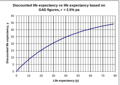
Figure 2 Discounted life expectancy versus life expectancy at r = 2.5% pa, based on ONS figures. ... 58
Figure 3 J = 1 indifference curve for income against (undiscounted) life expectancy. ... 59
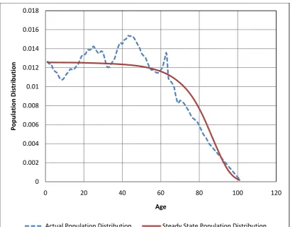
Figure 4 Population distributions calculated from UK data for 2007-2009... 80
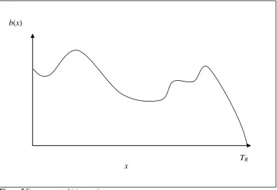
Figure 5 Exposure rate, b(x), over time, x. ... 111
Figure 6 Probability density for the mortality period, y. ... 111
Figure 7 The excess mortality probability distribution for radiation-induced cancer. ... 112
Figure 8 The excess mortality distribution for pollution-induced mortality. ... 112
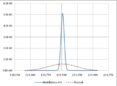
Figure 9 Probability distribution of the GDP per person estimate. ... 164
Figure 10 Historical data showing how the UK GDP and population size are correlated. ... 165
Figure 11 Life expectancy, Xd(a), and average life expectancy, Xd,. ... 166
Figure 12 Historical data showing the variation in the wage share of the GDP, θ, for the UK from 1955. ... 167
Figure 13 Time series data from the work time fraction, w0, the wage share of the GDP, θ, and the risk aversion, ε, for available data from 1984 to 2008. ... 168
Figure 14 Normal-quantile plot for risk aversion normality test. ... 169
Figure 15 Values of the age dependent VTPF, and the age-averaged VTPF, for discount rates 0% and 2.5%. ... 170
Figure 16 Values of the VODLY and VODLYA, for discount rates of 0% and 2.5%. ... 171
Figure 17 Result of Pearson’s chi-square test for 24 tests. ... 186
Figure 18 Difference between the linear approximation and the exact calculation of the change in life expectancy, as a function of the hazard rate.. ... 187
Figure 19 Rectangular distributions for gw(t), pw(t) and pw(t)gw(t) ... 188
Figure 21 Response of the reluctance to invest (R120A) with increasing risk aversion
(ε), for different normalised costs of the safety system (-0.1 < b < 0.6). ... 201
Figure 22 The derivative of the reluctance to invest when ε = 0.5 and c = 0.9, illustrating the two roots of the objective function g(ε, b) = 0. ... 202
Figure 23 The derivative of the reluctance to invest when ε = 0.9 and c = 0.999, illustrating the two roots of the objective function g(ε, b) = 0. ... 203
Figure 24 The derivative of the reluctance to invest when ε = 1.5 and c = 0.9, illustrating the single root of the objective function g(ε, b) = 0. ... 204
Figure 25 The derivative of the reluctance to invest when ε = 1.5 and c = 0.999, illustrating the single root of the objective function g(ε, b) = 0. ... 205
Figure 26 Dose received by individual of age a who is undergoing scans at future age t. ... 215
Figure 27 The response of the additional risk faced by an individual of current age a at future age t.. ... 216
Volume II
Figure 28 Fuel chain (from top to bottom) and construction materials chain (from left to right) used in the analysis. Arrows indicate transportation processes. ... 37Figure 29 Diagram of current and new build risk and output levels. Current impacts = R1/O1, future impacts = R2/O2 and incremental impacts = ΔR/ΔO. ... 38
Figure 30 Incremental immediate occupational risks for each technology. ... 144
Figure 31 Incremental immediate public risks for each technology. ... 145
Figure 32 Incremental delayed occupational risks for each technology. ... 146
Figure 33 Incremental delayed public risks for each technology. ... 147
Figure 34 All incremental immediate risk for each technology. ... 148
Figure 35 All incremental delayed risk for each technology. ... 149
Figure 36 All incremental occupational risk for each technology. ... 150
Figure 37 All incremental public risk for each technology... 151
Figure 38 All incremental normal operation risk for each technology. ... 152
Figure 39 All incremental abnormal operation risk for each technology. ... 153
Figure 40 Total incremental risk for each technology. ... 154
Figure 42 Public and occupational risk proportions of total impacts... 166
Figure 43 Immediate and delayed risk proportions of total impacts. ... 167
Figure 44 Normal and abnormal operation risk proportions of total impacts. ... 168
Figure 45 Comparison of immediate occupational fatality risks. ... 169
Figure 46 Comparison of delayed occupational fatality risks. ... 170
Figure 47 Comparison of immediate public fatality risks. ... 171
Figure 48 Comparison of delayed public fatality risks. Note the logarithmic scale. ... 172
Figure 49 Comparison of total risk. Note the logarithmic scale. ... 173
Figure 50 Relationship between power utility risk aversion, εp, and the Atkinson risk aversion, εA. ... 215
Figure 51 Exponential trend lines used in the extrapolation of the collective loss of life expectancy from CWP and silicosis. ... 225
List of Tables
Volume I
Table 1 Summary of literature on valuation of mortality risks. ... 36
Table 2 Hazard rate perturbations for limiting exposure and response distributions, assumed to be uniform over the specified period... 113
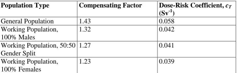
Table 3 Values of the compensating factor and dose-risk coefficient for different populations, using latest data. ... 113
Table 4 Data for the normal-quantile plot to test the risk aversion for normality. .. 172
Table 5 Results of the normal-quantile plot. ... 172
Table 6 Values of parameters ... 173
Table 7 Life expectancy under different population distributions. ... 190
Table 8 Work-life expectancy under different population and working time distributions. ... 190
Table 9 Work-time fraction under different population and working time distributions. ... 190
Table 10 Risk aversion under different population and working time distributions. The wage share θ is taken as 0.563, which was calculated for 2008 data. ... 190
Table 11 Deaths avoided and life-years gained for the four exposure limits from HSE’s assessment of methods to reduce occupational exposures to respirable crystalline silica. ... 217
Table 12 Cost of scheme and J-values using Table 11 data. ... 217
Table 13 Data for DH’s proposal to implement COMARE’s recommendations. ... 217
Table 14 Data for DH’s proposal to reduce the number of MRSA deaths. ... 217
Table 15 Loss of life expectancy to public and workers following a notional large nuclear accident. ... 218
Volume II
Table 16 Summary of literature on UK comparative risk analyses. ... 23Table 17 HGV statistics, from [62], [63] and [64]. ... 59
Table 18 Train freight and passenger statistics, from [65] and [153]. ... 59
Table 19 Rail fatalities 2005-2009, from [152] and [153]. ... 59
Table 21 UK production of stone, from [25]. ... 60
Table 22 UK production of minerals, from [25]. ... 60
Table 23 UK production of selected manufactured materials, from [25]. ... 61
Table 24 Quantities of recycling and waste production, from [58] and [59]. T ... 61
Table 25 HSE fatality statistics for extractive industries classed under “other mining and quarrying”. ... 62
Table 26 HSE fatality statistics for extractive industries classed under “mining of coal and lignite; extraction of peat”. ... 62
Table 27 UK offshore fatalities, 2006 – 2010, see Table 86 for further details. ... 63
Table 28 HSE fatality statistics under classification “basic metals” in manufacturing section. ... 63
Table 29 HSE fatality statistics under classification “non-metallic mineral products” in manufacturing section. ... 63
Table 30 HSE fatality statistics attributed to recycling of metals and non-metals, and for waste the wholesale and treatment of waste. ... 64
Table 31 PM2.5 emissions for manufacturing industries, and collective exposures, from [56], [57] and [158]. ... 65
Table 32 PM2.5 emissions for extractive and disposal industries, and collective exposures, from [56] and [57]. ... 65
Table 33 PM2.5 emissions from transportation processes, from [56] and [57]. ... 66
Table 34 Summary of impacts associated with extraction processes, in terms of years of lost life expectancy/Mt ... 67
Table 35 Summary of manufacturing, waste disposal and recycling impacts. ... 67
Table 36 Summary of impacts associated with the steel material chain. ... 68
Table 37 Summary of impacts associated with the concrete material chain. ... 69
Table 38 Summary of impacts associated with the copper material chain. ... 70
Table 39 Summary of impacts associated with the lead/zinc material chain. ... 71
Table 40 Summary of impacts associated with the aluminium material chain. ... 72
Table 41 Summary of impacts associated with the glass material chain. ... 73
Table 42 Summary of impacts associated with the plastic material chain. ... 74
Table 43 Construction, operation and decommissioning dates of UK nuclear facilities, including assumed dates for reference facilities. ... 93
Table 45 Assumptions used for new nuclear plants. ... 96
Table 46 Areva employment figures, 2004 – 2009. From [3], [4], [5], [6]. ... 96
Table 47 Areva fatality figures, 2004 – 2009. From [3], [4], [5], [6]. ... 96
Table 48 Areva global market share and inferred global average fatalities ... 96
Table 49 Uranium mines output, safety data and exposure rates. ... 97
Table 50 Exposure rates at the preparation stage. ... 97
Table 51 Predicted collective doses arising from emissions of radionuclides for the EPR and AP1000 new PWR reactors. ... 97
Table 52 Employment and doses to the workforce. ... 98
Table 53 Public collective doses. ... 100
Table 54 AP1000 Release frequencies and resulting collective doses. See [201]. .. 101
Table 55 Data for reference large nuclear accident. ... 101
Table 56 Material requirements for new build. ... 102
Table 57 Current hazard elimination premiums for various impacts arising at different fuel chain stages. ... 103
Table 58 Incremental hazard elimination premiums for various impacts arising at different fuel chain stages. ... 104
Table 59 Operation and decommissioning lifetimes of UK coal facilities, including assumed lifetimes for reference facilities, and capacities, capacity factors and remaining output from 2010 to 2070. ... 114
Table 60 Operation and decommissioning lifetimes of UK gas CCGT facilities, including assumed lifetimes for reference facilities, and capacities, capacity factors and remaining output from 2010 to 2070. ... 116
Table 61 Assumed construction, operation and decommissioning lifetimes of new CCGT and coal plants, and assumed capacity and capacity factors. ... 117
Table 62 Occupational collective doses. ... 117
Table 63 Public collective doses. ... 117
Table 64 Particulate matter emissions from E.On UK coal plants. New Build plant is assumed to operate at full load. ... 118
Table 65 Particulate matter emissions from E.On UK gas plants. ... 118
Table 86 UK Energy fatalities between December 2005 – November 2010. Major
data sources: [1], [40], [103], [104], [131]. ... 229
Table 87 UK generation of electricity by the assessed technologies. Data from [49]. ... 230
Table 88 UK production of natural gas [48]. ... 230
Table 89 UK production of oil [46]. ... 230
Acknowledgements
First and foremost, I would like to thank my supervisor, Professor Philip Thomas for the tremendous support that he has given me over the course of my research. He has provided me with much help and knowledge whilst still allowing me a great degree of personal autonomy which I feel has been invaluable in enabling me to develop and grow my research into something I can feel proud of. Without his patience, encouragement, assistance and tireless effort, this thesis would not have been possible. For this and much more, I am deeply grateful.
I would also like to thank Dr. Willie Boyle for his inestimable help and for the numerous enlightening discussions which have produced many interesting and sometimes fruitful avenues for our research. He has also provided great assistance on some of the more technical issues that I have been faced with over the past three years. He has been an ever present source of support and I could not wish for a kinder or more friendly colleague.
Professor Dick Taylor has also helped and supported me in countless ways, for which I express my gratitude. His insightfulness and understanding has enabled me to provide focus to my research. He has devoted much time into aiding me and providing feedback as I developed my research. I consider myself extremely fortunate to have been able to draw upon his experience and knowledge of both industry and academia.
I am also grateful to have had support from so many other distinguished colleagues. Roger Jones has always been willing to patiently listen and provide feedback. Geoff Vaughan’s experience has provided an invaluable bridge between academia and industry. His knowledge of the technical issues that are of real concern to industry and regulators has shaped my research and given it perspective and relevance that it otherwise would not have had. Ian Waddington has also helped and in many areas and we have had many thoughtful discussions that have been very beneficial.
Francois and Debbie Hodges have always shown great ability in being able to find and book for me meeting rooms, sometimes at late notice. Ferdie Carty has also provided essential technical support.
I thank the EPSRC and for funding my studies.
I also express my gratitude to Sing Gin and Caroline for their help in lending me their laptop when all other computers had failed me.
I also thank my parents, Chris and Diane for the incalculable support they have given me through all of my studies at university.
Declaration
The author declares that this thesis and the work presented in it is his own and has been generated by him as the result of his own original research.
Abstract
This thesis presents and extends the J-value framework for assessing expenditure on risk mitigation, and then applies the method in a comparative risk assessment of UK electricity generating systems.
The thesis is split into two volumes. The first volume contains part one, in which the J-value framework is introduced and developed. The loss of life expectancy is a key parameter in the framework, and general risk models for calculating this parameter are developed in terms of exposures and responses. Specific examples of radiation and pollution models are also presented. The “Hazard Elimination Premium” is also introduced as a useful common metric for risk comparisons.
Part one also contains an assessment of the uncertainty of the J-value and its input parameters and it is found that the J-value has an internal accuracy of around 3%, but that other, context dependant parameters can degrade this accuracy. A sensitivity analysis of the J-value framework also found that the J-value was reasonably robust against random variation of the input parameters as well as against the use of simplifying assumptions used in the development of the J-value.
The second volume contains parts two and three. Part two describes the comparative risk analysis of the electricity generating systems. The analysis is carried out on nuclear, coal, natural gas, onshore wind and offshore wind. The analysis assesses human mortality impacts arising from the current and future plants over the sixty year period from 2010 to 2070 for the entire fuel chain. The results indicate that nuclear generally has the lowest impacts, while gas, onshore and offshore wind have indicative impacts that are about an order of magnitude greater, although the
estimates for both wind technologies carry considerable uncertainty. Coal power was found to present high impacts compared with the other technologies, mainly as a result of pollution emissions. Total nuclear impacts were found to be sensitive to assumptions regarding the use of collective dose and the assumptions which are then used to calculate impacts. For the most pessimistic case, when world exposures are taken, total nuclear impacts increase by about an order of magnitude, which would render the risks from nuclear generation comparable with those from gas and wind generation.
Nomenclature
List of Roman Symbols
Symbol Meaning Units
A Assets £
AP Productivity constant
a Age year
arec Recruitment age year
aret Retirement age year
B Cost of risk mitigation system £
B0 Risk-neutral maximum reasonable
spend on risk mitigation system
£
b Constant exposure rate additional deaths/year
ba Normalised cost of risk mitigation
system
bcoll Collective exposure rate additional man-deaths/year
bi Discrete value of normalised cost of
risk mitigation system
bmax Maximum normalised reasonable
spend on risk mitigation system
b(x) Exposure rate at time x additional deaths/year
btot(x) Total individual exposure
C Cost of accident £
c(a) Earnings per year at age a £/year
ca Normalised cost of accident
cT Total dose risk coefficient for
radiation exposures
Sieverts-1
D Difference in expected utilities
Da Number of deaths at age a
Df Linearised discount factor
D(t) Probability of dying before age t D(u1,u2|ε) Difference in initial and final utility at
given risk aversion ε
da Number of life table deaths at age a
dr(x) Annual radiation dose Sieverts/year
E Emission rate μgs-1
a
Eˆ Number of deaths calculated from survival proababilities based on specific model
E(u1) Initial expected utility
E(u2) Final expected utility
ea Life expectancy at discrete age a year
F Expected remaining free time year
F(a) Expected remaining free time at age a year
f0 Optimal free time fraction chose by
society as a whole
fd(t) Probability density for death year-1
fmale Fraction of population that is male
fM(y) Probability density that the excess
mortality resulting from a given exposure occurs at time y
year-1
fT(η) Total probability density for death at
time η
year-1
G GDP per person £/year
GC National GDP £/year
g(ba, ε) Derivative of reluctance to invest
g(x) Probability density for death at time x
from given exposure
year-1
gd(t|a) Probability density function for death
at age t given survival to age a.
year-1
gw fraction of time spent working for
average person in work
gw(t) Fraction of time spent working for
average person of age, t, and in work
H Population entropy
HT Total man-hours worked in all
populations
hours
Hw(t) Total man-hours worked at age t hours
h(a) Hazard rate at age a year-1
hw(t) Individual hours worked at age t hours
J Judgement value
Jp(x) Jump function for response to
exposure
JT Total judgement value
J2 Second judgement value
K Capital investment per person £
KC National capital investment £
k Expected number of accidents as used in the Poisson distribution
krad Distributed radiation risk coefficient year-1
kpoll Pollution risk coefficient μg-1m3
k1 Constant
k2 Constant
LC National labour supply man-year
la Number of life-tables survivors to age
a
ma Discrete central rate of mortality at
age a
mamale Male central rate of mortality at age a
mafemale Female central rate of mortality at age
a
mr.max Maximum risk multiplier
N Number of people affected by protection system
NC Number of people in a country
NPop Total size of a given population
Npy Annual person-years worked
na Mid-year population at age a
n(a) Size of population at age a
nw(t) Number of people working at age t
O Electrical energy output Gigawatt-year (GWa)
pL Price of labour £/year
p(a) Population density at age a year-1
psw(t|a) Probability for being employed at age
t given survival to age a
year-1
pw Average probability of being in work
for all persons of working age
pw(t) Probability for being employed at age
t
year-1
p(y)λ Probability density of y accidents
occurring with frequency λ
p1 Initial no-accident probability
p2 Final no-accident probability
Q Life-quality index
Qf Life-quality index in terms of income
and free time fraction
Qf,d Discounted life-quality index in terms
of income and free time fraction f
Q Constant value of life-quality index on an indifference curve
QX Life-quality index in terms of income
and life expectancy
X
Q
Constant value of life quality index on an indifference curve Q1 Version of life-quality indexQ2 Version of life-quality index
q Elasticity parameter
qa Probability of death at age a
R(a) Expected utility for individual of age,
a
Rr Restoration requirement
Rr(a) Restoration requirement at age a
R120A Reluctance to invest
r Net discount rate year-1
rd Discount rate year-1
rg Growth rate year-1
survival to age a.
T Random age of death year
TR Release Period year
t Age, time year
tav Average age in a population year
tav2 Average square age in a population year2
tav3 Average cubed age in a population year3
ta+.ave Average age of those above age a year
tw.av Average working age year
U(G) Utility of income, G
u0(ε) Initial utility at risk aversion ε
VD(xd) Value of a delaying a fatality by xd
years
£
Vp(a) Value of temporarily preventing a
fatality for someone of age a
£
Vp Value of temporarily preventing a
fatality for someone of unknown age £
Vp.av Average value of temporarily
preventing a fatality
£
W(a) Cumulative hazard rate at age a w work-time fraction
w0 Optimal work-time fraction chosen by
society as a whole.
X Average life expectancy year
Xd Average discounted life expectancy year
X(a) Life expectancy at age a year
Xd(a) Discounted life expectancy at age a year
x Time year
xd Discounted delayed time until death year
Y Random number of accidents
y Time elapsed since induction year
yw Work-life expectancy year
yw(a) Work-life expectancy at age a year
zp Normal quantile function
zw(t|a) Fraction of time someone of age, a,
can expect to be working at age, t
List of Greek Symbols
Symbol Meaning Units
α1 Constant
β Constant
γ Constant
δbi Step size for normalised cost of
protection system
δc(x) Increase in concentration levels μg.m-3
δdis Discrimination limit
person's income as a result of spending on a health and safety scheme that will extend his life
δGN Maximum reasonable change in a
group of N people’s income as a result of spending on a health and safety scheme
£/year
δhabs(t|a) Absolute change in hazard rate at age t
given survival to age a.
year-1
δhrel(t|a) Relative change in hazard rate at age t
given survival to age a.
year-1
δVN Maximum reasonable spend on a
protection system for N people who will experience a gain in life
expectancy of Xd
£
N Vˆ
Actual spend on protection system. £
δW(t|a) Change in cumulative hazard rate at age t given survival to age a
Wˆ
Actual spend on risk protection system that protects against physical and financial risks
£
δXcoll Collective loss of life expectancy man-year
δXd Change in average discounted life
expectancy
year
δXd(a) Change in average discounted life
expectancy at age a
year
δZR Maximum reasonable spend on
financial risk mitigation systems
£
Zˆ
Actual spent on financial risk mitigation system
£
δε Step size for risk aversion
δχ(a) Change in random life to come at age
a
year
ε Risk aversion coefficient
εmax Maximum risk aversion
εpp Permission point
ηf Elasticity of free time fraction with
respect to income
ηMU Elasticity of marginal utility with
respect to income
ηX Elasticity of life expectancy with
respect to income
θ Share of wages in the GDP Λ(x) Number of deaths at time x λ Hazard rate when deaths are
exponentially distributed
year-1
νd(xd) Value of a discounted life-year £
νave Average value of a life-year £
π1 Initial accident probability
π2 Final accident probability
ρ Population density persons/m3
ρf,g Correlation coefficient between
parameters f and g
ζf Standard deviation for parameter f units of f
η Age year
ϕ0(y) Response function year-1
χ Random life to come when age is unknown
year
χ(a) Random life to come at age a year 2
1 k
Chi-square test statistic with k – 1 degrees of freedom
Φ-1
(p) Inverse normal cumulative distribution at value p
ψ0(x) Prolonged response function
ψ1(x) Integrated prolonged response function
ψ2(x) Twice integrated prolonged response
function
Ω Duration of long exposure year
ω1 Time to start of response to exposure year
ω2 Time to end of response to exposure year
List of Abbreviations
COE Compensation of Employees £/year
GDP Gross Domestic Product £/year
MI Mixed Income £/year
MRS Marginal rate of substitution
RR Relative risk
VODLY Value of a discounted life-year £
VODLYA Average value of a discounted life-year
£
VTPF Value of temporarily preventing a fatality
Chapter 1 Introduction
1.1 Statement of Problem
The purpose of the research contained in this thesis is to use the J-value framework to assess and compare the risks from diverse methods of electricity generation in the UK.
1.2 Aims and Objectives
The aims of this research are:
1. Validate the J-value framework as a suitable and robust tool for risk assessment and analysis.
2. Compare, in a consistent manner, the risks posed by various electricity generating systems in the UK using the J-value framework.
It is intended that these aims will be achieved through the following objectives: 1. Extending the existing framework by incorporating more general risk models
in the loss of life expectancy calculations, and conducting uncertainty and sensitivity analyses.
2. Use the J-value framework to develop a common metric that can be used to compare the risks from electricity generating systems on a consistent basis, i.e. in such a manner that does not bias the results towards any particular electricity generating system.
3. Develop a framework for the comparative risk analysis that will incorporate all relevant risks involved in the generation of electricity for each system in a manner that will ensure a fair and valid comparison.
1.3 Structure
historical context and existing literature in this field. The subsequent chapters then describe in detail the concepts and methods used in deriving the J-value, and develop them further. Areas in which the existing framework is developed further include:
A new derivation of the J-value through consideration of the trade-offs made at an individual and societal level.
Generalised relative and absolute risk models of the loss of life expectancy following any given exposure and response pattern. This model is also applied to the specific case of pollution risks.
A more rigorous treatment of the measurement and estimation procedures for the parameters used in the J-value framework, including an assessment of the tolerances to be placed on each parameter.
Introduction of the concept of a “Hazard Elimination Premium”, which is the maximum reasonable amount to spend to completely eliminate a hazard. The HEP is used extensively in the second part of the thesis.
A sensitivity analysis of the J-value framework, in which the robustness of the J-value given the initial assumptions and uncertainty of some of the input parameters is assessed.
The J-value has been recently extended by Thomas et al (2009, 2010) [190], [191], [192] to include mitigation of financial risks in addition to physical risks. These concepts come together to form a “total judgement value”, or JT-value. The model
behind this extension is shown, and the computational methods employed to calculate some of its outputs are also presented. Part one then concludes with some example calculations.
the overall results, comparisons with other studies and a discussion of the significance and limitations of the results.
Part 1 Valuing Health and Safety
Individuals have always traded risks to their health and life in order to obtain other benefits. These trades reflect how the individual values his or her life. In a modern democratic society, it is necessary to make decisions about public safety that invariably affects the health and the wealth of many individuals. There is now widespread consensus that any such method used to aid the decision making process regarding public safety should reflect as far as is possible the preferences which the individuals in a society place upon their safety. Any such method must be fully consistent in the way that risks are valued, and should also be transparent. Currently the most widespread method used for valuing risks are stated preference techniques used to elicit an individual’s willingness to pay (WTP) for a given risk reduction. The advantages and disadvantages of this method have been summarised in the preceding section. The purpose of this thesis is to describe a relatively new technique for valuing risks known as the “J-value” method, developed by Thomas et al (2006) [182], [183], and (2009) [188].
appropriately. A value for risk can then be inferred by insisting that any decision that changes a society’s average life expectancy and income (measured by the GDP per person) must at least preserve the initial LQI, and preferably increase it, i.e. the change in the LQI must not be negative. If a protection system is known to afford a given increase in life expectancy to a group of individuals, then the constraint on the change in the LQI places an upper bound on the amount of money that should be spent on implementing the scheme. This maximum value can then be taken as representing the societal cost of risk. If the actual cost of the protection system is known, then the J-value is the ratio of this cost to the societal cost. The J-value is therefore a dimensionless positive number. J-values of less than unity indicate that the protection system costs less than the maximum theoretical cost of risk, and so represent good value for money. Implementing these schemes will result in an increased LQI. J-values greater than unity indicate that the cost of the protection system is greater than the theoretical maximum, and hence should not be implemented. The J-value can be seen to be a scale on which safety projects and risk policies may be judged. The scale is universal, in the sense that it is not specific to any single industry, and all the input parameters are fully objective quantities, most of which are derived from reliable national and actuarial statistics. The J-value, being a single dimensionless number, is also transparent and easily interpreted.
The J-value framework has also been extended recently (2010) [192] to include financial risks to assets. This is formulated around an expected utility model, which can be used to determine objectively the risk preferences of the individual or organisation facing the risk, which can then be used to determine the maximum reasonable spend on eliminating the risk.
used to infer common metrics of the value of life, namely the value of temporarily preventing a fatality (VTPF), and the value of a discounted life-year (VODLY), and also introduces the “Hazard Elimination Premium” (HEP), which will be used extensively in part 2 of this thesis. Chapter 8 presents the measurements of all the necessary input parameters to the J-value, and also provides an assessment of the tolerance limits of the J-value. In chapter 9 a sensitivity analysis is performed to assess the robustness of the J-value to the underlying assumptions. Chapter 10 gives an introduction to the J2 and JT-values, and describes how the maximum reasonable
spend on financial risks can be determined. Finally, chapter 11 presents some example calculations, demonstrating the general nature and applicability of the J, J2
Chapter 2 Historical Context and Existing Literature
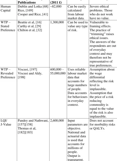
The valuation of health and safety schemes, proposals or policies must also reflect the value to be placed on physical risk, and consequently, the value placed on human lifespan. In this section, some of the historical and more recent literature of such valuations will be reviewed. Particular focus will be given to the various methodologies that have been used to value these risks. It is common practice to express risk valuations in terms of how much should be spent on avoiding one statistical fatality, a measure commonly known as the “value of a statistical life” or the “value of preventing a fatality”. However, the latter term is somewhat misleading, as preventing a fatality is in the long run impossible – all individuals will eventually die. It is for this reason that, for the purposes of this thesis, the term “Value of Temporarily Preventing a Fatality” (VTPF) will be used. Although there are many ways to calculate the VTPF, one of the most common methods is the following: if it has been determined that each member of a population of size N is willing to pay £v to eliminate a risk that has a probability of 1/N of killing each member, then an amount totalling £Nv is willing to be spent on eliminating a risk that is expected to kill one person. Therefore, the VTPF = £Nv. The VTPF is usually an input into health and safety decision making. However, this is not the case in J-value analysis – the risk valuation technique that is the main concern of this thesis – where the VTPF is an output that can be calculated if so required.
males of ages between 20 and 60 being deemed the most valuable, at 50 shekels of silver. Females of these ages were valued at thirty shekels. This would mean a VTPF of £412, and £247 respectively, using the same calculations as before. Individuals outside this age group had lower valuations.
The first formal research into the value of life came some three thousand years later, but used largely the same methods of valuation. The method of valuing human life in terms of an individual’s future productivity and earnings came to be known as the “human capital” method. Some of the first authors to investigate this method were Adam Smith in 1776 [176], and Ernst Engel in 1883 [74]. A more in depth historical review of human life valuation is provided by Dublin and Lotka (1930) [68], who also provide a calculation of a VTPF using this approach. They calculate the net future earnings of an individual to be approximately $9,802, in 1930 prices, or a VTPF of about £82,000 in 2011 prices. This approach suffers from some serious ethical problems, such as the zero value of retirees or those who do not work. Children are also assigned a relatively small valuation, due to the traditional economic method of discounting future earnings. According to Schulze (1980) [174], the early attempts at applying this method to value health and safety programs:
“Have given economists a “black eye” for supposedly advocating that individual human lives could be valued as the lost economic productivity associated with a shortened life span”
These problems have meant that there have been relatively few modern attempts at valuing physical risk using this method, the most notable being Rice (1967) [169], who used this approach to value the cost to society of illness, disability and death. A follow up to this study was published ten years later by Cooper and Rice (1976) [41]. Lave and Seskin (1970) [127] have also used this method to value the societal cost of air pollution.
to mitigate risks to society should reflect the degree to which the individuals are willing to pay to do so. Precisely how much an individual is willing to pay must be determined through techniques that can be classed as either “revealed preference” or “stated preference”.
Stated preference techniques have the advantage that they can be used to estimate the value of any type of risk. There are, however, a number of drawbacks. These include the tendency for the respondents to give inconsistent answers. For example, as briefly mentioned above, the same question can elicit different responses, depending on how the question was asked. This is known as the “framing effect”. Such studies also usually have to resort to “trimming”, whereby respondent’s answers are removed from the sample if the experimenter judges them to be either inconsistent or not representative of the sample as a whole. This process violates the ethical and democratic principle that all individual’s preferences should be accounted for with equal weight, and also undermines the fundamental principle that the VTPF should reflect the willingness to pay of society. Perhaps the most severe drawback of the stated preference technique is that there is little reason to suspect that an individual’s preferences for safety, when elicited in an isolated environment devoid of the vast array of factors that are confronted in everyday life, will be representative of how the individual makes decisions about his safety in reality.
individuals, and much of which is freely available. The techniques also reflect to some degree decisions based on real-world choices, as opposed to the isolated decisions elicited by the stated preference techniques discussed above. The disadvantages of these techniques are that the assumptions regarding wage differentials being caused by differing levels of safety, and the price of a risk reducing item being equal to the value of the risk, are implausible. Clearly, many factors can affect wage levels and prices. The assumption that employees make considered decisions about whether to take a job based only on wage and safety considerations is also doubtful. The difficulties of these assumptions are borne out by the large range of the VTPF calculated in this manner.
Another method of valuing physical risk that has been developed recently is based on the Life Quality Index (LQI) method, first developed in 1997 by Nathwani, Lind and Pandey [137], [157]. The LQI is a summary indicator that can be used to measure the development of a nation, based on its Gross Domestic Product (GDP) per person, and its average life expectancy. By insisting that any protection system at least maintains the initial LQI, a maximum reasonable cost for the system can be determined. This cost is then the societal value of the given risk reduction. The calculation involves using labour market data to infer how individuals prefer to distribute their time between working, in which income is raised, and leisure, in which the income is consumed. In this sense, the LQI method can be seen to be a revealed preference technique for determining the societal WTP for risk reductions.
cost-effectiveness of drugs, and radioactivity abatement systems. Much of the initial J-value research centred around radiation protection, in which the exposure to radiation and subsequent mortality response was stochastically modelled in order to determine the loss of life expectancy from a given exposure to ionising radiation, see Thomas et al (2006) [184], (2007) [185] and (2009) [186], [187].
Further recent developments of the J-value method include an extension of the method to include valuation of environmental risks (2010) [192], and an analysis of the tolerance of the J-value(2010) [123]. The main advantages of the J-value method are that the input parameters are objective, being estimated from actuarial or national statistics. The method is also transparent, the output being a simple dimensionless number that is easy to interpret. It is also consistent, offering a simple scale by which risks can be assessed. The disadvantages of the method are that it only values mortality risks, and cannot be used to assess morbidity, or non-fatal risks. Nor does the method account for the pain or suffering which may be experienced over the individual’s remaining lifespan, for example, by using “Quality Adjusted Life-Years” (QALYs) that are used in health economics.
Method Examples of Major Publications
VTPF (2011 £)
Advantages Disadvantages
Human Capital
Dublin and Lotka [68] Rice, [169]
Cooper and Rice, [41]
~82,000 Can be easily calculated from labour market data.
Severe ethical problems. Those who do not work have no value. WTP –
Stated Preference
Beattie et al, [16] Carthy et al, [29] Chilton et al, [32]
1,300,000 Can be used to value any type of risk.
Vulnerable to framing effects. The practice of “trimming” raises ethical issues. The answers of the respondents are out of everyday
context and may therefore not be representative of true preferences. WTP –
Revealed Preference
Viscusi, [197] Viscusi and Aldy, [198]
600,000 – 55,000,000
Uses reliable labour market data that accounts for large numbers of people. Data accounts for behaviours in everyday context.
Assumption about the wage
differential reflecting the risk level is
implausible. Assumption that the price of a risk reducing
commodity is equal to the value of the risk is also implausible. LQI/
J-Value
Pandey and Nathwani, [157][158]
Thomas et al, [182][183]
2,600,000 Input
parameters are objective. National and actuarial data is used that accounts for millions of people. Output is transparent.
[image:37.595.114.526.85.652.2]Does not account for morbidity risks or QALYs.
Chapter 3 Conceptual Foundations of the J-Value
3.1 The Life Quality Index
It is impossible to determine each and every factor required to ensure that the highest quality of life may be enjoyed by all individuals. There are a vast amount of variables that influence an individual’s welfare, and exactly what is entailed by a high quality of life is entirely subjective. Any rational analysis of such a complex and indeterminate concept must attempt to make an appropriate simplification by identifying the key factors which underlie the concept of quality of life. It is postulated that the quality of life of an individual can be distilled into two fundamental factors: how long an individual can expect to live from now on, and how much the individual has available to spend, both on life’s necessities and on its luxuries. The first of these factors is encapsulated in the life expectancy, X, which is measured in years. This factor may be distilled further by recognising that individuals generally enjoy their life during time that they are free to dispose of as they wish, in contrast to time that is spent working.
For many people, the distinction between working time and free time is an arbitrary one, as people often engage in productive work even though they are not compelled to do so. Nevertheless, individuals will generally wish to retain flexibility over how they choose to spend their time. The productiveness of a society may be viewed as the result of a complex trade-off that each individual makes between working time and free time. In this trade-off the benefit gained from extra income obtained by working longer hours is balanced against the cost of loss of free time. This suggests that a more precise indicator of quality of life can be obtained by replacing the life expectancy with the remaining average free time, F, where:
wXF 1 (3.1)
within the nation is treated equally with regards to income. Thus, free time and average income are taken as being the two main inputs contributing to the single output of quality of life. In economic theory, inputs are related to outputs through a “production function”, the most common of which is the Cobb-Douglas production function, (see e.g. Johansson (1991) [117]). If the output is denoted, Q1, and
represents a “life quality index” of an average person, then G and F are related to Q1
by:
G
F
Q
1
1 (3.2)where α1, β and γ are dimensionless positive constants. A property of the
Cobb-Douglas function is that any monotonic increasing function of Q1 will also suffice as
a life quality index. This property is then used to define a second life quality index,
Q2:
wX
GF G Q
Q q q
1
1
1 1 2
(3.3)
where q = β/γ is a dimensionless positive constant, and where equation (3.1) has been used in the last step. It may also be noted that the work time fraction is the complement of free time fraction, f:
w
f 1 (3.4)
which allows equation (3.3) to be recast as:
fX
G
Q
q (3.5)where Q is used instead of Q2, as this is the most general form for the life quality
the amount of money available to spend over this time. The potential for trade-offs between these three factors will now be considered. Firstly, it is assumed that free time fraction and life expectancy cannot be substituted. However, there are some very low values of f which would be associated with a reduced level of life expectancy due to overwork. This presumably is not an issue for most individuals. It therefore seems reasonable to assume that f and X are independent of one another. Two important trade-offs remain, however. These are the trade-off an individual can make between income and free time fraction, i.e. between G and f, and the trade-off between income and life expectancy, i.e. between G and X, which occurs when spending on a risk reducing protection scheme, or indeed, accepting compensation for a reduced life expectancy (for example via higher wages in a high risk job).
Consideration of these trade-offs leads to the concept of a maximum reasonable spend on safety and protection systems. This then allows a judgement or J-value to be assigned to such a system, which can be expressed as a single equation. Although the J-value has been derived before from different principles (e.g. see Thomas et al (2006a) [182]), the following is a new derivation based upon standard economic theory2. The independence of f and X means that the two tradeoffs described above can be considered separately, as will be done in the following sections.
3.2 The Trade-Off between Free Time Fraction and Income
In exploring the free time fraction-income trade-off, it is assumed that any such trade does not affect the individual’s life expectancy. This means that a new life quality index, Qf, can be formed by dividing the original life quality index, equation (3.5),
by X, without loss of generality:
f
G
X
Q
Q
f
q (3.6)This new life quality index is introduced in order that the features of the trade-off can be explored explicitly. It is apparent from equation (3.6) that it is possible for an
2
individual to exchange his income for free time, whilst still retaining his original life quality index. The set of values of G and f that will render a constant level of life quality, which will be denoted as Qf , is known as an “indifference curve”, as it is assumed that the individual is indifferent to how his level of life quality is attained. The indifference curve must satisfy:
f G
Qf q (3.7)
which can be solved for f or G. Here it will be solved for G, to obtain:
q q f f Q
G 1
1
(3.8)
One property of equation (3.8) is that there are an infinite number of indifference curves, with each one representing a different level of life quality. Also, none of these indifference curves intersect one another. The indifference curve is also convex, meaning that the function will always lie below a straight line drawn between any two points on the line. Convexity of indifference curves directly implies a diminishing marginal rate of substitution (MRS) of free time fraction for income. This is the amount of income that must be exchanged for a unit of free time fraction, and is given as:
qf
G qf
Q df dG
MRS q
q
f
1 1
1
(3.9)
Equation (3.9) clearly shows that the MRS diminishes with increasing levels of free time fraction. The implication of a diminishing MRS is that the higher the free time fraction enjoyed by the individual, the less willing the individual will be to give up some income in order to increase free time fraction further.
This is done by again using a Cobb-Douglas production function, following Pandey et al (2006) [158]. The output in this instance is the national GDP, denoted as GC,
and the factors of production are the national capital investment, KC, and the annual
supply of labour within the country, LC:
C C P
C A K L
G 1 (3.10)
where AP is a productivity constant, that accounts for other factors affecting
production, such as technological advancements and education level. The other parameter θ is the fraction of the GDP paid to workers as wages, as will now be shown:
The price of labour, pL, is the marginal GDP with respect to labour supply, at
constant levels of productivity and capital, i.e.:
C C
C C L
L G dL
dG
p (3.11)
so that:
C C L
G L p
(3.12)
The numerator in equation (3.12), which is the product of the price of labour and the labour supply, is the total wages paid to employees. Thus equation (3.12) shows that
θ is the wage share of the GDP.
Furthermore, the supply of labour may be seen to be equal to the total population of a country, NC, multiplied by the population-averaged work-time fraction:
f
N
w
N
where equation (3.4) has been used in the last step. Substituting into equation (3.10) gives:
f N K A
GC P C1 C 1 (3.14)
The GDP per person, G, is then:
f AK
f N
K A N G G
C C P C
C
1
1 1
1
(3.15)
where K is the capital investment per person.
Equation (3.15) shows that average income is related both inversely and non-linearly to the free time fraction. This curve is a constraint that is determined by the collective actions of individuals within a society and links the average individual’s income to his free time fraction. It will now be assumed that these collective actions of a society will be such that the life quality is maximised for the average individual, subject to the above constraint. The maximisation occurs when the indifference curve defined by equation (3.8) is tangent to the constraint curve defined by equation (3.15). This situation is demonstrated in Figure 1, which presents data relevant to UK conditions in 2007. This figure shows the downwards curving income constraint, and the convex indifference curves. These three curves represent different levels of the life quality index, Qf. The highest curve gives the highest quality of life. This
If the point of tangency is located at (f0, G0), then the derivative of the indifference
curve is given by the negative of equation (3.9), evaluated at these points:
0 0 , 0
0 qf
G MRS df
dG
G f
(3.16)
The derivative of the constraint line of equation (3.15) is:
0 0 , 0 1
0 f
G df
dG
G
f
(3.17)
Matching the derivatives of (3.16) and (3.17) gives:
0 0 0
0
1 f
G qf
G
(3.18)
which can be solved for q, the only unknown parameter. This gives:
0 0 0
0
1 1 1
1
w w f
f q
(3.19)
where, clearly, f0 = 1 – w0. The meaning of the parameter q may be further explored
by rearranging equation (3.9) to give:
f
dG df f G
q (3.20)
which is valid for dG/df > 0. The parameter ηf is the income elasticity of free time
3.3 The Trade-Off between Income and Life Expectancy
The second trade-off investigated is between income and free time fraction. The nature of this trade-off is different from the first trade-off, which was determined by a collective bargaining process made at a societal level. The trade-off between income and life expectancy occurs when health and safety schemes are being considered. Such a health and safety scheme can be expected to improve life expectancy by a certain amount, but at a cost. This cost may be borne by each individual in society, even if the individual does not directly benefit from the health and safety improvement, in line with the compensation notions of Kaldor (1939) [120] and Hicks (1939) [92] (see also Boadway and Bruce (1984) [21] and Johansson (1991) [117]).
The income-life expectancy trade-off is assumed to be independent of the free-time fraction. This means that a new life quality index, QX, may be formed, in a similar
manner to equation (3.6), by dividing the general life quality index given by equation (3.5) by f, which is now being treated as a constant, rather than as a variable. Hence:
X G f Q
QX q (3.21)
As is the case with the first trade-off, it is possible for an individual to give up some income for additional life expectancy, whilst still retaining his initial level of life quality. It is also clear that excessive spend on life expectancy improvement will reduce the individual’s life quality, whilst suitably small spends will increase life quality. Thus the maximum reasonable spend for a health and safety scheme defines the indifference curves for this trade-off. The set of values of G and X that define the indifference curve at a constant level of life quality, denoted as QX , must satisfy:
X G
QX q (3.22)