Primon : the implementation of a software monitor : a thesis presented in partial fulfilment of the requirements for the degree of Master of Science in Computer Science

PRIMON:

The Implementation of a Software Monitor

by

Anthony James McGregor

A thesis presented in partial fulfilment of the requirements for the degree of

Master of Science in Computer Science

at

Massey University

ABSTRACT

ACKNOWLEDGEMENTS

I would like to thank,

Tom Docker, my supervisor, particualarly for his efforts

while criticising the many drafts of this thesis, and

Table of Contents

Introduction ...•...•.•••....•.•.••..••...•...•.•.•..•••••••••••• 1 2 An introduction to computer performance evaluation •••••••••••••••••• 9 2. 1 Monitors •••.•••••••••••.••••••••.•••••••••••••.•••••••••••••••• 12 2.2 Models ••••••••••••••••••••••••••.•••••••••••••••••••••••••••••• 15

3 The

3.

3.3

principles of software monitoring •••••••••••••••••••••••••••••• 25 The structure of software monitors ••••••••••••••••••••••••••••• 25 Performance indices ....••...•...••.•••....••. 27

Measuring disciplines •••••••••••••••••••••••••••••••••••••••••• 28

3.3.1 Event trapping•••••••••••••••••••••••••••••••••••••••••••30 3.3.1.1 Collecting the data •••••••••••••••••••••••••••••• 31 3.3.1.2 Recording the data ••••••••••••••••••••••••••••••• 31 3.3.1.3 Problems with event trapping ••••••••••••••••••••• 33 3.3.1.3.1 Access •••••••••••••••••••••••••••••••••••••• 33 3.3.1.3.2 Overheads ••••••••••••••••••••••••••••••••••• 34

3.3.1.3.3 Sensitivity •.•••••••••••.••••••••••••••••••• 34

3.3.2 (Random) 3.3.2.1

Sampling • ••••••••••••••••••••••••••••••••••••••• 35 Collecting the data •••••••••••••••••••••••••••••• 36 3.3.2.1.1 Collecting data by unit workloading ••••••••• 41 3.3.2.1.1.1 Advantages of unit workloads ••••••••••• 42 3.3.2.1.1.2 Disadvantage of unit workloads ••••••••• 43 3.3.2.2 Recording the data ••••••••••••••••••••••••••••••• 43 3.3.2.3 Advantages of random sampling •••••••••••••••••••• 44 3.3.2.3.1 Reducing distortion ••••••••••••••••••••••••• 44 3.3.2.3.2 Simplicity of installation •••••••••••••••••• 46 3.3.2.4 Problems with random sampling •••••••••••••••••••• 46 Reporting the results of monitoring •••••••••••••••••••••••••••• 47 3.4.1 Quoting the indices•·•••••••••••••••·••••••••••••••••••••48 3.4.2 Tables•••••·••••••••••··•••····•••••·•·••••·••••••••••••·48 3.4.3 Histograms••·••••••••••••••••••••••••••••••••••••••••••••49 3.4.4 Gantt profiles ••••••••••••••••••••••••••••••••••••••••••• 50 3.4.5 Kiviat graphs •••••••••••••••••••••••••••••••••••••••••••• 52

4.1.11 I/Os per second and page faults per second •••••••••••••• 64 4.1.12 I/0 trace•••••••••••••••••·••·••••••••••••••••••••••••••64

4.1.13 Page out trace•••••·•••••••••••·••••·•••·•••••••••••••••65

4.2 Inappropriate measures••••••••••••·••••••••••••••••••••••••••••65 4.2.1 Memory utilisation·••·••··•··••••••••••••••••••••••••••••65 4.2.2 Number of processes in memory••••••••••••••••••••••••••••65

4.3 Difficult measures···••••••••·•·•···•••·•••••••••••••••••••••••66

4.3.1 Number and source of interrupts••••••••••••••••••••••••••66

5 Primon•••••••••••••••••••••••••••••••••••••••••••••••••••••••••••••68 5.1 Features•••••••••••••••••••••••••••••••••••••••••••••••••••••••70 5.2 Development •••••••••••••••••••••••••••••••••••••••••••••••••••• 71

5.3 XREF•••••••••••••••••••••••••••••••••••••••••••••••••••••••••••74 5.4 The monitors .•••••••••.•••••.••••.•.••••••••••••••••••••••••••• 76

5.5

5.4.1 Interactive queue length monitor•••••••••••••••••••••••••77 5.4.1.1 Purpose•·••·•••••••••••••••••••••••••••••••••••••77

5.4.1.2 Background ••••••••••••••••••••••••••••••••••••••• 77

5.4.1.3 Implementation•••••••••••••••••••••••••••••••••••78 5.4.1.4 Distortion and integrity considerations •••••••••• 79 5.4.2 Validation.••••••••••••••••••••••••••••••••••••••••••••••79

5.4.2.1 Known variations•••••••••••••••••••••••••••••••••80 Batch

5.5.1 5.5.2

5.5.3

5.5.4

queue length monitor••·••••••••••••••••••••••••••••••••••81 Purpose••••••••••••••••••••••••••••••••••••••••••••••••••81 Implementation ••••••••••••••••••••••••••••••••••••••• ~ ••• 82 5.5.2.1 Reports••••••••••••••••••••••••••••••••••••••••••82

5.5.2.1.1 Distortion and integrity considerations ••••• 85

5.5.2.2 Validation ••••••••••••••••••••••••••••••••••••••• 86

5.5.2.2.1 Known variations.••••••••••·••••••••••••••••87 Disk activity monitor••••••••••••••••••••••••••••••••••••89 5.5.3.1 Purpose••••••••••••••••••••••••••••••••••••••••••89 5.5.3.2 Background•••••••••••••••••••••••••••••••••••••••90 5.5.3.3 Implementation ••••••••••••••••••••••••••••••••••• 91 5.5.3.4 Reports••••••••••••••••••••••••••••••••••••••••••94 5.5.3.5 Testing••••••••·•••••••••••••••••••••••••••••••••97

5.5.3.6 Validation ••••••••••••••••••••••••••••••••••••••• 97

Relative availability monitor••••••••••••••••••••••••••••98 5.5.4.1 Purpose••••••••••••••••••••••••••••••••••••••••••98

5.5.4.2 Background ••••••••••••••••••••••••••••••••••••••• 98

5.5.4.3 Implementation••••••••••••••••••••••••••••••••••100

The sampler.•••••••••••••••••••••••••••••••101

5.5.4.3.1

5.5.4.3.1.1 The loosely coupled sampling

function•••••••••••••••••••••••••••••••••••••••101 5.5.4.3.1.2 The mini-benchmarks•••••••••••••••••••102 5.5.4.3.2 The reducer••••••••••••••••••••••••••••••••105 5.5.4.3.3 The plotter.•••••••••••••••••••••••••••••••105 5.5.4.3.4 The calibrator•••••••••••·•••••••••••••••••107

5.5.4.4 Testing•••••••••••••••••••••••••••••••••••••••••107 5.5.4.5 Validation •••••••••••••••••••••••••••••••••••••• 110

5.6.3 Disk record positioning•·•••••••••••••••••••••••••••••••115 5.7 Evaluation of Primon••••••••••••••••••••••••••••••••••••••••••118

6 Conclusions ••••••••••••••••••••••••••••••••••••••••••••••••••••••• 120

Appendix A

Appendix B

1 Introduction

Computer Performance Evaluation (CPE) has developed both as an

academic and an applied subject of considerable importance, as

witnessed by its mention in Discussion Paper 3 for the recent Brownlie

Committee report [BROW82]. As an applied discipline CPE is used

primarily in the areas of

o computer design and development

o capacity planning and

o system tuning.

A need for access to CPE tools can be identified when administering

most computer systems and to this end a range of tools is available on

most (large) computers. Prime computers are a notable exception and

several groups involved with Prime equipment have shown a desire for

access to CPE tools. These groups include computer centres, who wish

to improve the performance of the computer systems under their

control, researchers in CPE, and teaching staff who wish to

demonstrate the use of performance evaluation.

This thesis reports on the implementation of one such tool called

Primon. We begin in chapters two and three by discussing CPE in

general and measurement in particular. Following this, in chapters

four and five we discuss the specific area of measuring Prime

computers and the implementation of Primon. Finally in chapter six we

review the development of Primon and suggestions made in previous

chapters for further work that could usefully be undertaken. Details

of the architecture and systems software of Prime systems are

contained in Appendix A, and the program listings for Primon are given

in Appendix B.

2 An introduction to computer performance evaluation

The performance evaluation of computer systems has become widespread

because of the high cost and complex nature of modern computers.

As an example of the use of CPE consider a computer system operated by

Superior Operational Software (SOS), a fictitious software company

writing system software for Prlme computers. The system functions

well until the number of interactive users exceeds a threshold. The

System Administrator is faced with the task of raising this threshold,

while remaining within a strict capital budget.

He may proceed as in Figure 2.1 with a CPE study. The aim of the

study will be to identify the reasons for the current threshold, and

it is hoped that this will lead to an informed decision being made on

whether the performance can be improved by tuning the operating system

constants which the System Administrator has access to (e.g.the length

of the time slice, size of buffers etc) or whether the system will

need to be upgraded to meet requirements (capacity planning).

I V

Performance Problem

I

l(CPE Study)

I

I

---.

Problem Identified Problem not Identified

I

I

I

I

I

I

I

I

I

.---A--->

available)! I

j(Tuning / Capacity Planning)

I

V

Problem solved.

Example use of CPE Fig 2.1

This type of scenario is common but is by no means the only use of

CPE. Performance questions also arise when designing new systems, or

when choosing a new or replacement system. Hopefully a company

installing a computer system for the first time will want to be

satisfied that the proposed system will have sufficient capacity to

process the workload within an acceptable time frame. A manufacturer

designing a new machine may have specified design criteria which

include instruction execution rate improvements over a previous model.

Performance Evaluation is used in these situations as well.

From the above discussion it is clear that CPE studies are performed

on many types of system, and have a wide range of objectives. This

has led to a range of tools to be developed for use in CPE. Many of

these tools have been developed for a particular CfE project, while

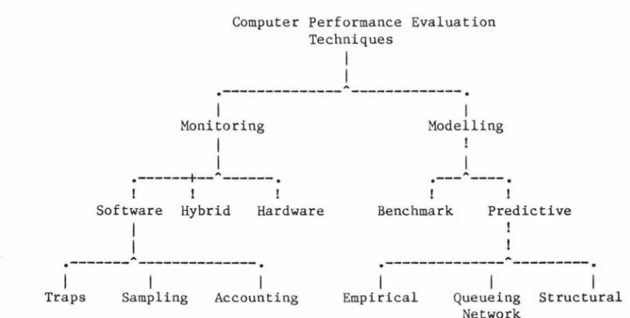
others are Operations Research techniques. Fig 2.2, and the rest of

this chapter, describe some of the more common techniques and their

relationships to one another. Other categorizations are possible and

some techniques are also known by other names.

A specific monitoring tool could be made up of more than one of these

techniques. For an example see the hybrid model of [SCHW78].

Computer Performance Evaluation Techniques

Monitoring

I

I

.---+--A---.

A

I

I

I Modelling

I

Benchmark Predictive

.---

---.

.--- ---.

Traps Sampling Accounting Empirical

The CPE tree Fig 2.2

11

Queueing Network