Designs for generalized linear models with several variables and model uncertainty

Designs for Generalized Linear Models with Several Variables and

Model Uncertainty

D.C. Woods _and S.M. Lewis Southampton Statistical Sciences

Research Institute School of Mathematics University of Southampton Southampton SO17 1BJ, UK ([email protected])

([email protected])

J.A. Eccleston Center for Statistics School of Physical Sciences

University of Queensland Brisbane QLD 4072, Australia

([email protected])

K.G. Russell

School of Mathematics and Applied Statistics University of Wollongong

Wollongong NSW 2522, Australia ([email protected])

Standard factorial designs may sometimes be inadequate for experiments that aim to estimate a generalized linear model, for example, for describing a binary response in terms of several variables. A method is proposed for finding exact designs for such experiments which uses a criterion that allows for uncertainty in the link function, the linear predictor or the model parameters, together with a design search. Designs are assessed and compared by simulation of the distribution of efficiencies relative to locally optimal designs over a space of possible models. Exact designs are investigated for two applications and their advantages over factorial and central composite designs are demonstrated.

KEY WORDS: Binary response; D-optimality; Logistic regression; Robust design; Simulation.

1. INTRODUCTION

The most common type of planned experiment in scientific and industrial research is one in which the design for the experiment is the “best” choice when the observations are adequately described by a linear model. Experiments sometimes take place which use such designs when this assumption is not justified. An important example is when a combination of values of the explanatory variables, or treatment, is applied to each unit and a binary response is observed; either a “success” or a “failure”. A design that is efficient under a linear model may then be inadequate for obtaining accurate description, prediction and understanding of the system under investigation, even when the experimental data are analyzed using an appropriate nonlinear model, such as a generalized linear model. Particular circumstances when this problem may arise include experiments in which the probability of success is near 0 or 1 for one or more of the treatments, see Cox and Reid (2000, p.180).

Sections 3 and 5, where it is shown that the methods in this paper have advantages over the use of standard factorial designs. A further example from our own consulting is an investigation by a food manufacturing company, Dalgety plc, into the use of protected atmosphere packing to give peeled potatoes a shelf-life of one week. This experiment studied the effect of three quantitative variables, namely, vitamin concentration in the pre-packaging dip and the levels of two gases in the packing atmosphere, on several binary responses including the presence or absence of liquid in the pack after seven days. In Section 7, we demonstrate the advantage of using a design obtained by the proposed methods compared with the central composite design used by the experimenters. Further industrial experiments where a generalized linear model described the response were discussed by Myers, Montgomery, and Vining (2002).

Research to date on the generation of designs tailored for generalized linear models has concen-trated mainly on simple models with only one or two explanatory variables; see, for example, Minkin (1987), Chaloner and Larntz (1989) and Sitter and Torsney (1995). For larger numbers of variables, Torsney and Gunduz (2001) extended the work of Ford, Torsney, and Wu (1992) to several variables but the results obtained do not lead to a general method for the generation of designs. Where more than one variable may jointly affect a response, theoretical results are scarce and have not resulted in generally applicable methods for the generation of optimal de-signs. A flexible algorithmic approach is needed that allows a range of models to be considered, together with an appropriate method of evaluating design performance.

The key difference between the design of experiments for linear and for nonlinear models is that, for nonlinear models, initial estimates of the model parameters must be available from previous studies or scientific understanding, in order to allow an optimal design to be constructed. Three approaches to finding a design using such estimates are: Bayesian methods, described by Chaloner and Larntz (1989), Chaloner and Verdinelli (1995) and Firth and Hinde (1997), a sequential approach developed, for example, by Abdelbasit and Plackett (1983), Wu (1985) and Minkin (1987), and the use of a minimax criterion, see, for example, Sitter (1992) and King and Wong (2000). A review of design methods for generalized linear models was given by Atkinson and Haines (1996).

less computational effort than a minimax or a fully Bayesian method, particularly when several variables are to be investigated. The algorithms for finding and assessing the designs, writ-ten in C++, are available from http://www.maths.soton.ac.uk/staff/woods/glm design, together with supplementary material.

2. GENERALIZED LINEAR MODELS

Suppose an experiment involves f explanatory variables and a set of design points xj =

(x1j, . . . , xf j), for j = 1, . . . , n, where −1 ≤ xij ≤ 1 is the value of the ith variable at the jth design point and thendesign points are not necessarily distinct. The distinct design points are called the treatments in the experiment or, alternatively, the support points of the design. It is assumed that the units in the experiment are exchangeable, in the sense that the distri-bution of the response to a treatment does not depend on the unit to which the treatment is applied, and that one observation Yj is made on each unit. The observations are assumed to be independent and described by a generalized linear model; see McCullagh and Nelder (1989) or Myers et al. (2002). Such models have three components: (i) a distribution of the response, (ii) a linear predictor, and (iii) a link function g(.) that relates the mean response E(Yj) =µj

to the linear predictor

η=Xβ, (1)

where β = (β0, . . . , βq−1)′ is a vector of unknown parameters, X is an n×q matrix of known

functions of the f explanatory variables andη is ann×1 vector with jth element ηj =g(µj). For a given distribution for the response, a choice of link function is often available. If the response variable at the jth design point has a Bernoulli distribution with success probability

πj =g−1_{(ηj), then a widely used link function is the logit or logistic link}

g(πj) = log

πj

1−πj

, for j = 1, . . . , n. (2)

Alternative link functions for Bernoulli data include the probit link g(πj) = Φ−1_{(πj), where}

Φ−1 is the inverse of the cumulative distribution function of the standard normal distribution, and the complementary log-log link g(πj) = log [−log(1−πj)]. The methods described here may be applied to the wide class of generalized linear models including, for example, a Poisson response with log link function. They are demonstrated in this paper for binary and binomial responses.

Suppose that a design d for a generalized linear model s = (g,η,β) consists of t treatments, where the kth treatment is applied tomk units (k = 1, . . . , t) chosen at random. The assump-tion of independent observaassump-tions and exchangeability of units allows the number of successes observed on the kth treatment to be modeled by a binomial(mk, pk) distribution, where pk is the probability of success when the kth treatment is applied to a unit.

The maximum likelihood estimators ofβ(from (1)) have asymptotic variance-covariance matrix that is the inverse of the Fisher information matrix

M(d, s) = X′W X , (3)

d. For Bernoulli data, the weights are

w(xj) =

dπj dηj

2

/{πj(1−πj)}.

For example, w(xj) = πj(1−πj) for the logistic link function.

For a generalized linear model, a locallyD-optimal design minimizes the volume of the asymp-totic confidence ellipsoid for the model parameters or, equivalently, maximizes the objective function

φD(d, s) = ln|M(d, s)|1/qs

, (4)

where qs is the number of parameters in s.

For a given model s, we define the local efficiency under D-optimality of a particular design d

relative to a locally optimal design dl as

eD(d, dl;s) = exp

φD(d, s)−φD(dl, s) . (5)

We assess the performance of a design through the distribution of its local efficiency over a set of models. The same approach may be applied to any nonlinear model.

3. PERFORMANCE OF FACTORIAL DESIGNS

When an initial screening experiment is being planned, a lack of detailed prior knowledge about the generalized linear model may preclude the use of a locally optimal design. Experimenters then often use two-level factorial or fractional factorial designs which are readily available and are efficient under linear models. Such designs do not require initial parameter estimates but their performance for parameter estimation and prediction is still determined by the unknown values of the model parameters and varies across the parameter space. This property may lead to poor performance in some regions of the parameter space as illustrated in this section.

Suppose that f variables are to be investigated in an initial study using a design d0 composed

of m replicates of a factorial or fractional factorial design. Suppose also that a first-order or “main effects only” linear predictor is assumed for the jth design point given by

ηj =β0+ f

X

i=1

βixij, for j = 1, . . . , n . (6)

The response variable for thekth treatment is assumed to follow a binomial(m, pk) distribution, where pk is related to the model parameters βi (i= 0, . . . , f) through the logit link.

In order to assess the performance of designd0asβ = (β0, . . . , βq−1)′ takes values in a parameter

space B ⊂ Rq_{, where q =f + 1, the distribution of its local efficiency (5) is approximated as}

Table 1: Ranges of each model parameter for the parameter spaces Bj (j = 1,2,3)

Parameter space

Parameter B1 B2 B3

β0 [-3,3] [-1,1] [-3,3] β1 [-2,4] [0,2] [4,10] β2 [-3,3] [-1,1] [5,11]

β3 [0,6] [2,4] [-6,0]

β4 [-2.5,3.5] [-0.5,1.5] [-2.5,3.5]

(i) A sample ofn0 parameter vectors, β, is drawn at random from B.

(ii) For each vector

(a) a design ds is found that maximizes φD_{(d, s), and}

(b) the local efficiency eD_(d

0, ds;s) of the design d0 is calculated, from (5).

The above approach is now used to investigate the design d0 for f = 4 factors, composed of m= 3 replicates of the 2f _{factorial treatments (±1, . . . ,±1), which is a possible design for the}

crystallography application. The performances of this design are assessed and compared for the three parameter spaces B1, B2 and B3, defined in Table 1, using a sample of n0 = 10,000

parameter vectors. Here B2 has the same centroid asB1 but substantially smaller volume, and

B3 has the same volume asB1 but is centered further from (0, . . . ,0).

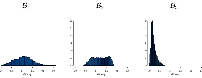
Figure 1 shows the distribution of the relative efficiency of d0 for each of the three spaces. For

B1, the design has median efficiency of 0.43 and lower quartile 0.31. The minimum efficiency

of almost 0 indicates that, for certain β values, very little information is available for the es-timation of the parameters by maximum likelihood. The concern that a design may lead to data from which maximum likelihood estimates cannot be obtained was addressed by Silva-pulle (1981) and, for sequential design, by Wu (1985). It can be investigated by the approach of Hamada and Tse (1996) or, more feasibly for large experiments, through simulation. For d0

andβ located at the centroid of the spaceB1, the probability of the non-existence of maximum

likelihood estimates is approximately 0.77. There is therefore a high chance that an alternative method would have to be used to analyze the data. The method of Firth (1993), based on pe-nalized likelihood, guarantees finite parameter estimators with smaller bias than the maximum likelihood estimators and the same asymptotic variance-covariance matrix. Hence maximiza-tion of (4) remains an appropriate criterion for design choice for this analysis method. This method is applied in Section 7 to the potato packing experiment.

The distribution of the efficiency of the factorial design varies according to the parameter space. For example, the efficiency distribution of d0 for B2 compared with the corresponding

distribution for B1 has smaller spread, a higher median (0.48) and a larger minimum (0.16),

as shown in Figure 1. The worst performance of the factorial design is for B3 which has the

B1 B2 B3

efficiency

0.0 0.2 0.4 0.6 0.8 1.0

0

2

4

6

8

10

12

efficiency

0.0 0.2 0.4 0.6 0.8 1.0

0

2

4

6

8

10

12

efficiency

0.0 0.2 0.4 0.6 0.8 1.0

0

2

4

6

8

10

12

Figure 1: Histograms of the efficiency of the 24 _{factorial design relative to locally optimal}

designs for each of the parameter spaces B1, B2 and B3.

4. COMPROMISE DESIGN SELECTION CRITERIA

The above example demonstrates the need for designs that take account of uncertainty in the values of the parameters in the linear predictor. Further uncertainty in a generalized linear model may arise from the choice of link function or from the functional form of the linear predictor; for example, whether first or second order is appropriate. We represent uncertainty in the models= (g,η,β) through setsG, (N |g) and (B |g,η) of possible link functions, linear predictors and model parameters, respectively. This formulation allowsη to depend on g, and the model parametersβwithin the linear predictor to depend on bothg andη. The sets may be incorporated into a general criterion for design selection that maximizes an objective function ΦI obtained by integrating or averaging a local objective function φ(d, s) across a model space

Mto give

ΦI(d,M) =

Z

g

Z

η|g

Z

β|g,η

φ(d, s) dh1(β|g,η) dh2(η|g) dh3(g), (7)

where M = {(g,η,β) :g ∈ G,η∈(N |g),β∈(B |g,η)} and h1, h2 and h3 are appropriate

cumulative distribution functions. In practice, G and (N |g) will often be finite sets and the corresponding Stieltjes integrals in (7) are then evaluated as summations. In some applications of the criterion, (B |g,η) is also a finite set, as illustrated in Section 6.

The maximization of (7) is a generalization of the average criterion of Fedorov and Hackl (1997) which includes only uncertainty in β. Pettersson and Nyquist (2003) found optimal designs under the average criterion for generalized linear models where only a fixed and finite choice of possible values is allowed for each variable. The concept of compromise criteria can, in fact, be traced back to Stigler (1971) who considered polynomial regression models. Further work on this idea for linear models includes that of Atkinson and Cox (1974), Studden (1982), Cook and Nachtsheim (1982) and Cook and Wong (1994).

The evaluation of ΦI for design selection is mathematically intractable and hence numerical

methods must be used. When designs involve several variables, the usual deterministic and Monte Carlo methods (see, for example, Evans and Swartz (2000)) are too computationally intensive for incorporation within a search algorithm. Hence we use a surrogate for (7), namely,

Φ(d,S) =X

s∈S

where S ={(g,η,β) :g ∈ S1,η∈(S2|g),β∈(S3|g,η)}, for the finite sets

S1 ⊂ G, (S2|g)⊂(N |g) and (S3|g,η)⊂(B|g,η), and wherep(s) is a probability mass function.

The set S is chosen to represent the model space M, as described in the following sections. Similar criteria for uncertainty in linear models have also been considered by L¨auter (1974, 1976) and Dette and Studden (1995). When the approach is viewed from a Bayesian perspective as, for example, by Zhou et al. (2003), it may exhibit the dichotomy discussed by Etzioni and Kadane (1993) and, most recently, by Han and Chaloner (2004), that different prior distributions are used for design and analysis.

Under D-optimality, that is whenφ =φD _{from (4), it is not necessary to adjust (8) to scale for}

the maximum obtainable value ofφD _{achieved by locally optimal designds for eachs∈ S. This}

is because a design that maximizes (8), that is, maximizes ΦD(d,S) =P

s∈Sp(s) ln|M(d, s)|/qs, will also maximize

exp ΦD(d,S) =Y

s∈S

|M(d, s)|p(s)/qs

. (9)

Since M(ds, s) does not depend on d, the same choice of design will maximize the geometric mean Q

s∈S

|M(d, s)|p(s)_{/|M(ds, s)|}1/qs

. The maximization of (9) requires less computation than the alternative of maximizing a weighted sum of efficiencies

X

s∈S

p(s)

|M(d, s)| |M(ds, s)|

1/qs

, (10)

as it does not require locally optimal designs to be obtained. We have found that the difference between the performances of designs found via (9) and (10) is small when they are assessed using the method and model spaces of Section 3. This situation is analogous to that of exactD- and

A-optimal designs for a linear statistical model, where the objective functions are respectively geometric and arithmetic means of eigenvalues of the information matrix.

Throughout this paper, D-optimality is employed and a uniform probability mass function is assumed for p(s). If certain generalized linear models were believed to be more appropriate than others, then a distribution that assigns greater weight to those models would be used. A design that maximizes (8) will be called a compromise design with respect to φ, S and p(s). Such designs are obtained and compared with alternative designs where there is uncertainty in the model parameters (Section 5) and in the form of the linear predictor and/or the link function (Sections 6 and 7).

5. COMPROMISE ACROSS A PARAMETER SPACE

In the early stages of an investigation, a design is needed to detect those variables that have a substantial effect on the response. A design might then be sought which performs well under a model with a first-order linear predictor (6) and a fixed link function. This was the situation for the crystallography example described in Section 1.

Suppose that the experimenters provide feasible, possibly wide, ranges of values for each model parameter. These ranges identify a spaceB ⊂ Rq _{of plausible model vectors where, for}

Parameter Set

Fraction plus centroid Centroid Coverage

P ar am et er S p ac e B1 efficiency

0.0 0.2 0.4 0.6 0.8 1.0

0

2

4

6

efficiency

0.0 0.2 0.4 0.6 0.8 1.0

0

2

4

6

efficiency

0.0 0.2 0.4 0.6 0.8 1.0

0 2 4 6 B2 efficiency

0.0 0.2 0.4 0.6 0.8 1.0

0

2

4

6

efficiency

0.0 0.2 0.4 0.6 0.8 1.0

0

2

4

6

efficiency

0.0 0.2 0.4 0.6 0.8 1.0

0 2 4 6 B3 efficiency

0.0 0.2 0.4 0.6 0.8 1.0

0

2

4

6

efficiency

0.0 0.2 0.4 0.6 0.8 1.0

0

2

4

6

efficiency

0.0 0.2 0.4 0.6 0.8 1.0

0

2

4

6

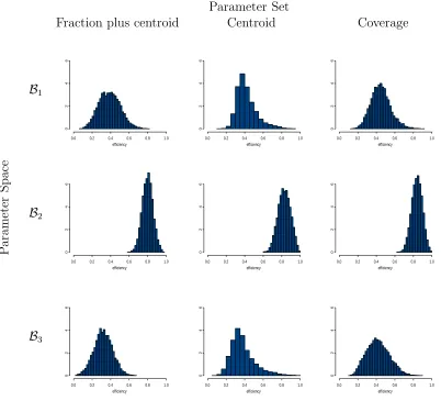
Figure 2: Distributions of efficiencies of nine compromise designs for three parameter spaces and three parameter sets.

whereS3 is a finite set of parameter vectors withinB that is chosen to representB. Thus there

are three stages to finding a “parameter compromise” design: (i) definition of the parameter space B, (ii) choice of a subset S3 of size n1, and (iii) search for the design.

We now apply this method to the four variable crystallography example to find designs com-posed of three replicates of 16 design points under a logistic regression model, using the pa-rameter spaces of Section 3 for illustration. We compare compromise designs found from the following choices of S3:

S31: A 25−2 resolution III fraction, where the levels of factor i are the limits of the βi range,

augmented by the centroid of B to given1 = 9 terms in (8).

S32: The centroid ofBalone, that is, the locally optimal design for the center of the parameter

space; this is a degenerate compromise design withn1 = 1.

S33: A coverage, or U-optimal, set of n1 = 9 parameter vectors obtained from a candidate set

of 65 _{equally-spaced points acrossB (see Johnson, Moore, and Ylvisaker, 1990).}

For each parameter space Bj, j = 1,2,3, a compromise design was found for each set of

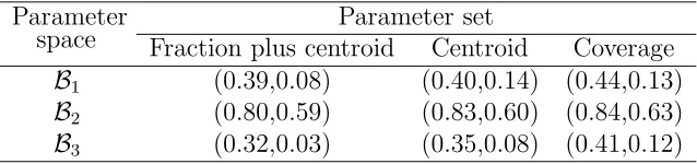
Table 2: Median and minimum local efficiencies for compromise designs found from three sets of parameter vectors under parameter space Bj (j = 1,2,3)

Parameter

space _{Fraction plus centroid}Parameter set_{Centroid Coverage}

B1 (0.39,0.08) (0.40,0.14) (0.44,0.13)

B2 (0.80,0.59) (0.83,0.60) (0.84,0.63)

B3 (0.32,0.03) (0.35,0.08) (0.41,0.12)

paper, are available at the website. Each of the nine designs was assessed for the parameter space for which it was constructed using the method of Section 3. The distributions of the local efficiencies in Figure 2, having median and minimum efficiencies given in Table 2, indicate that design performance varies with parameter space. The designs forB2, the space of smallest

volume, have the highest median and minimum efficiencies and the smallest variation in effi-ciency for each parameter set. The designs perform better across B1, which has centroid closer

to (0, . . . ,0), than across B3.

For each space Bj, the design obtained from using the 25−2 fraction plus centroid has poorer

performance than the locally optimal design found from the centroid alone. This finding sug-gests that the locally optimal designs for parameter values at the vertices of a parameter space are poor representatives of the uncountably infinite number of locally optimal designs for the entire space. The designs obtained from the coverage set S33 generally produced better

perfor-mances than those from S31 and S32, with the greatest improvement occurring for B3, which

has large volume and is centered furthest from (0, . . . ,0). Each compromise design has higher minimum efficiency than that of the 24 _{design d}

0 of Section 3 for each of the three parameter

spaces, with the most dramatic improvements in the efficiency distribution obtained for designs found for space B3 (see Figures 1 and 2). The minimum local efficiencies of the two designs

found from the centroid and from the coverage sets for B3 both exceed the median efficiency

achieved by design d0 for space B3.

From the above study and other examples, we recommend that, when the suggested ranges for the βi are not large, then a reasonable choice of design for an initial experiment is a locally optimal design found for the midpoints of the ranges of the parameter values. (The assessment software can be used to gauge the meaning of ‘large’ for a particular application). When the

βi ranges are large, and particularly when some are centered away from zero, a compromise design found from a coverage set may offer a better local efficiency distribution and will usually perform better than a factorial design.

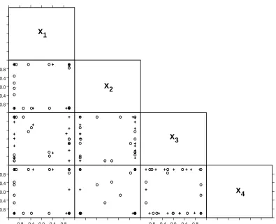
The two-dimensional projections in Figure 3 show the distinct combinations of variable values for the compromise designs forB1 found from S31, the fraction plus centroid, and from S33, the

coverage set. Both designs have a greater number of distinct values for each variable than d0.

The design found from S33 has more points in the extremes of the region than the S31 design

and a better performance across B1 for (8) under D-optimality. The tendency for D-optimal

designs to have points mainly concentrated in the extremes of the design region is well known for linear models.

-1.2 -0.8 -0.4 0.0 0.4 0.8

-1.2 -0.8 -0.4 0.0 0.4 0.8

-1.2 -0.8 -0.4 0.0 0.4 0.8 -1.2 -0.8 -0.4 0.0 0.4 0.8

x

x

x

x

Figure 3: Two-dimensional projections for compromise designs for B1 found from the fraction

plus centroid (◦) and the coverage set (+).

design in which each variable has somewhat fewer distinct values may be preferred by exper-imenters. Such a design may be obtained by replacing variable values that are close together by their average to give a slightly sub-optimal design.

A further way of selecting a design for the example is to allow the algorithm to find the best allocation d∗ of the 48 design points. This is a larger, more complex and more time-consuming optimization problem. The speed of the search and the efficiency of the resulting design are greatly improved by the use of a starting design dr composed of three replicates of

the corresponding compromise design for 16 runs, instead of a random starting design. The gain in performance of d∗ compared with dr can be quite small. For example, when designs d∗ anddrare found forB1 using the coverage set, a comparison of their performances by evaluation

of the ratio h(dr, d∗, s) = exp

φD_{(dr, s)−φ}D_(d

∗, s) , for a sample of 10,000 parameter vectors fromB1, gives a ratio greater than 1 for about 50% of the sample and first and third quartiles

of 0.93 and 1.04 respectively; in fact,dr has the best performance, relative to d∗, of any design composed of ureplicates of v runs such thatuv= 48.

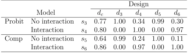
effective-Table 3: Efficiencies calculated from (5) of a compromise design dc and four locally optimal designs di under models si (i= 3, . . . ,6), where Comp denotes complementary log-log

Design

Model dc d3 d4 d5 d6

Probit No interaction s3 0.77 1.00 0.34 0.99 0.30

Interaction s4 0.80 0.00 1.00 0.00 0.97

Comp No interaction s5 0.64 0.99 0.24 1.00 0.11

Interaction s6 0.86 0.00 0.97 0.00 1.00

ness of the method is assessed and, in Section 7, its benefits are demonstrated for the potato packing experiment.

Example: Suppose there are two explanatory variables and uncertainty in whether an

inter-action term should be included in the linear predictor. The set N then consists of

η(1) =β0(1)+β (1)

1 x1+β2(1)x2 (11)

and

η(2)=β₀(2)+β₁(2)x1 +β2(2)x2+β3(2)x1x2. (12)

Then B |η(1)

={β(1)} and B |η(2)

={β(2)}, where β(1) = (β₀(1), β₁(1), β₂(1))′ _and

β(2) = (β₀(2), β₁(2), β₂(2), β₃(2))′_{. Suppose that initial estimates of β}(1) _{and β}(2) _{are available and,}

for simplicity, that a single logit link functiong is considered. The model spaceMthen consists of only two models, so thatS =Mwith elements s1 = (g, η(1),β(1)) ands2 = (g, η(2),β(2)).

A design dc that achieves a compromise in performance across the linear predictors is found by maximizing the objective function (8) for S = M and its performance is assessed through local efficiencies (5) for s1 and s2. For example, for designs with n = 6 points under

mod-els (11) and (12), if β(1) = (3.0,1.6,4.1)′ _{and β}(2) _{= (1.2,1.7,5.4,−1.7)}′_{, a design search finds} a compromise design with efficiencies 0.88 and 0.89 relative to d1 and d2, respectively.

Suppose that, in addition, there is uncertainty in whether the probit or complementary log-log (comp) link is appropriate. There are then four models in S, namely, s3 = (probit, η(1),β(1)), s4 = (probit, η(2),β(2)), s5 = (comp, η(1),β(1)), s6 = (comp, η(2),β(2)). Table 3 shows that

a compromise design enables estimation of all four models with efficiencies of at least 0.64. The locally optimal designs for the two models with first-order linear predictors do not allow models with an interaction to be fitted. The locally optimal designs for the models including the interaction can be used to estimate all four models. However, they have poor efficiencies (0.11-0.34) for estimating the first-order models. It is clear that the link function is less important than the form of the linear predictor in the performance of the designs for these parameter values.

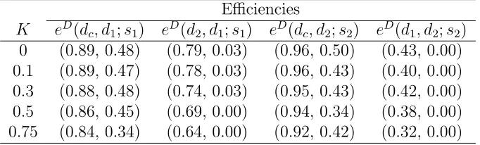
Table 4: Median and minimum values of the efficiency distributions for compromise designsdc

and locally optimal designs d1 and d2 for respective models s1 and s2 for various values ofK

Efficiencies

K eD_{(dc, d}

1;s1) eD(d2, d1;s1) eD(dc, d2;s2) eD(d1, d2;s2)

0 (0.89, 0.48) (0.79, 0.03) (0.96, 0.50) (0.43, 0.00) 0.1 (0.89, 0.47) (0.78, 0.03) (0.96, 0.43) (0.40, 0.00) 0.3 (0.88, 0.48) (0.74, 0.03) (0.95, 0.43) (0.42, 0.00) 0.5 (0.86, 0.45) (0.69, 0.00) (0.94, 0.34) (0.38, 0.00) 0.75 (0.84, 0.34) (0.64, 0.00) (0.92, 0.42) (0.32, 0.00)

variety of values of β(1) and β(2) by the following simulation procedure, which is defined and illustrated for compromise over s1 and s2. The steps are:

(i) A set ofn0 values ofβ(2) is drawn from a specified distribution.

(ii) Values forβ(1)are chosen to capture the fact that the removal of an interaction term from a linear predictor is likely to change or perturb the values of the remaining parameters, but not necessarily by large amounts. Hence, for each draw of β(2), the value of β(1) is obtained as β_j(1) = β_j(2)+zj, where zj ∼ N(0, σ2

j0) (j = 0,1,2) and σj0 = |Kβj(2)|, where

| · | denotes absolute value. This dependence of the variation in the perturbation on the size of the realized coefficients in model s2 (see (12)) gives a higher chance of greater

perturbations on larger, than on smaller, coefficients.

(iii) For each choice of values of β(1) and β(2), a compromise design dc and locally optimal designs d1 and d2 are each found by search and assessed through the local efficiencies eD_{(di, dj;sj) fori∈ {c,1,2}, j = 1,2, i6=j.}

The above procedure is illustrated for values of β(2) drawn from anMN(0, σ2_Iq

s

2×qs

2)

distribu-tion, where qs2 = 4 is the number of terms in the larger model and σ2 = 6 is used to produce

fairly wide ranges of parameter values. Table 4 gives the median and minimum efficiencies for the various compromise designs and locally optimal designs for models s1 and s2, for a choice

of values of K and n0 = 10,000. It shows that the compromise designs are more robust to the

choice of model than the individual locally optimal designs, with median efficiencies of 0.84 -0.89 for s1 and 0.92 - 0.96 for s2. (This is not surprising as the performance of locally optimal

designs is known to be sensitive to the choice of model). The locally optimal designs are also more sensitive to the value of K; for example, for designs found under s1 (s2), the decrease in

the median efficiency for estimating model s2 (s1) between K = 0 and K = 0.75 is 0.15 (0.11);

the corresponding decrease for the compromise designs is only 0.05 (0.04).

7. POTATO PACKING EXAMPLE

package available for R (R Development Core Team, 2006), gives the parameter estimates and standard errors shown in Table 5.

Usually, a pilot experiment would be used to obtain approximate ranges of the variables to be explored and preliminary parameter estimates. In our investigation, we use the estimates given in Table 5 to find a 16 run compromise design d†

c that incorporates uncertainty in whether

the form of the linear predictor is first-order (η(1)_{), first-order plus all two-variable interactions}

(η(2)_{) or full second-order (η}(3)_{); that is, compromising acrosssi = (logit, η}(i)_,β(i)_{), fori= 1,2,3.}

Table 6 gives the efficiencies (5) relative to the locally optimal designdi for model si, ford†c and

for the central composite designda. The compromise design has corresponding local efficiencies that are 36.7%, 111.8% and 44.6% larger than those for da. Its minimum efficiency (0.72) is, in fact, greater than the maximum efficiency (0.60) of the CCD across the models; estimation of the largest model (s3) is not possible for d1 and d2.

To investigate whether the advantage of a compromise design over the CCD is maintained across a variety of parameter values, a simulation was performed for the modelss1–s3, similar to that

of Section 6. For each of 10,000 iterations, a value of β(3) was drawn from a multivariate normal distribution with a mean vector whose elements are the parameter estimates for s3,

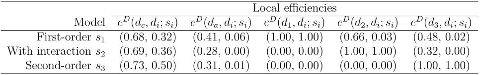
and diagonal variance-covariance matrix containing the corresponding estimated variances, see Table 5. Values forβ(2) and β(1) were obtained usingK = 0.3 in perturbations ofβ(3) andβ(2), respectively. The summary of the simulation results in Table 7 shows that, under each modelsi, the compromise design performs better than the CCD, with the minimum efficiency exceeding the median efficiency for the CCD under both s2 and s3. The results again demonstrate the

weakness of locally optimal designs under model uncertainty.

The advantage of the compromise design over the CCD is due to the use of prior information on the parameters but this information may be inaccurate. For the potato packing example, we can examine the impact of inaccuracies on the relative performance of d†

c compared with

the CCD by using the 10,000 simulated sets of parameter values (models) which, for s3, are

centered close to the parameter estimates from Table 5. For each of the 10,000 parameter draws, the relative efficiency h(da, d†c, si), defined in Section 5, was calculated. It was found

Table 5: Potato packing experiment: penalized likelihood parameter estimates and standard errors (S.E.) for the parameters in each of the models s1–s3

First-order s1 With interaction s2 Second-order s3

Term Estimate S.E. Estimate S.E. Estimate S.E. Intercept -0.28 0.57 -1.44 1.13 -2.93 1.98

x1 0 0.67 0 0.88 0 0.73

x2 -0.76 0.72 -1.95 1.32 -0.52 0.76

x3 -1.15 0.75 -2.36 1.38 -0.79 0.71

x1x2 – – 0 1.05 0 0.86

x1x3 – – 0 0.99 0 0.86

x2x3 – – -2.34 1.47 -0.66 0.86

x2

1 – – – – 0.94 1.18

x2

2 – – – – 0.79 1.18

x2

Table 6: Local efficiencies of a compromise design d†

c, a central composite designdaand locally

optimal design di under models si (i= 1,2,3) using parameter values from Table 5

Design Model d†

c da d1 d2 d3

First-order s1 0.82 0.60 1.00 0.91 0.70

With interaction s2 0.72 0.34 0.37 1.00 0.29

Second-order s3 0.81 0.56 0.00 0.00 1.00

Table 7: Median and minimum local efficiencies for compromise designs dc, a central composite design da and locally optimal designs di under model si (i= 1,2,3)

Local efficiencies Model eD_{(dc, di;si) e}D_{(da, di;si) e}D_(d

1, di;si) eD(d2, di;si) eD(d3, di;si)

First-order s1 (0.68, 0.32) (0.41, 0.06) (1.00, 1.00) (0.66, 0.03) (0.48, 0.02)

With interaction s2 (0.69, 0.36) (0.28, 0.00) (0.00, 0.00) (1.00, 1.00) (0.32, 0.00)

Second-order s3 (0.73, 0.50) (0.31, 0.01) (0.00, 0.00) (0.00, 0.00) (1.00, 1.00)

that, under s1 and s2, design dc† has a clear advantage with median values for h(da, d†c, si) of

0.68 and 0.62, respectively; while for the second-order model s3, the median value is 1.01.

8. DISCUSSION

A method of finding exact designs has been presented for use with generalized linear models with several explanatory variables. The method takes account of uncertainties in some, or all, of the model parameters, the form of the linear predictor and the link function. The advantages of the proposed method over the application of standard designs have been demonstrated through considering experiments in crystallography and food technology. An investment in preliminary runs to obtain rough estimates of parameter values leads to a substantial increase in the information gained from subsequent experiments compared with standard designs.

ACKNOWLEDGEMENTS

This work was supported by EPSRC e-Science grant GR/R67729 (Combechem). It benefited from visits by John Eccleston and Ken Russell to the Southampton Statistical Sciences Research Institute (S3_{RI), with the former supported by EPSRC grant GR/S85139. We are grateful}

to Mike Hursthouse (Director of the ESPRC National Crystallography Service, University of Southampton) for helpful discussions and to Mary Garratt and Peter Border for supplying details of the potato packing experiment.

REFERENCES

Abdelbasit, K. M. and Plackett, R. L. (1983), “Experimental Design for Binary Data,”Journal of the American Statistical Association, 78, 90–98.

Atkinson, A. C. and Cox, D. R. (1974), “Planning Experiments for Discriminating Between Models (with discussion),” Journal of the Royal Statistical Society, Ser. B, 36, 321–48.

Atkinson, A. C. and Fedorov, V. V. (1975), “The Design of Experiments for Discriminating Between Two Rival Models,” Biometrika, 62, 57–70.

Atkinson, A. C. and Haines, L. M. (1996), “Designs for Nonlinear and Generalized Linear Models,” inHandbook of Statistics, Vol. 13, eds. S. Ghosh and C. R. Rao, New York: Elsevier Science, pp. 437–475.

Chaloner, K. and Larntz, K. (1989), “Optimal Bayesian Design Applied to Logistic Regression Experiments,” Journal of Statistical Planning and Inference, 21, 191–208.

Chaloner, K. and Verdinelli, I. (1995), “Bayesian Experimental Design: A Review,” Statistical Science, 10, 273–304.

Cook, R. D. and Nachtsheim, C. J. (1980), “A Comparison of Algorithms for Constructing Exact D-optimal designs,” Technometrics, 22, 315–324.

— (1982), “Model Robust, Linear-Optimal Designs,” Technometrics, 24, 49–54.

Cook, R. D. and Wong, W. K. (1994), “On the Equivalence of Constrained and Compound Optimal Designs,” Journal of the American Statistical Association, 89, 687–692.

Cox, D. R. and Reid, N. (2000), The Theory of the Design of Experiments, Boca Raton: Chapman and Hall/CRC.

Dette, H. and Studden, W. J. (1995), “Optimal Designs for Polynomial Regression when the Degree is not Known,”Statistica Sinica, 5, 459–473.

DuMouchel, W. and Jones, B. (1994), “A Simple Bayesian Modification of D-optimal Designs to Reduce Dependence on an Assumed Model,”Technometrics, 36, 37–47.

Etzioni, R. and Kadane, J. B. (1993), “Optimal Experimental Design for Another’s Analysis,” Journal of the American Statistical Association, 88, 1404–1411.

Evans, M. and Swartz, T. (2000), Approximating Integrals via Monte Carlo and Deterministic Methods, Oxford: Oxford Science Publications.

Fedorov, V. V. and Hackl, P. (1997), Model-Oriented Design of Experiments, New York: Springer.

Firth, D. (1993), “Bias Reduction of Maximum Likelihood Estimates,” Biometrika, 80, 27–38.

Firth, D. and Hinde, J. P. (1997), “Parameter Neutral Optimum Design for Non-Linear Mod-els,” Journal of the Royal Statistical Society Ser. B, 59, 799–811.

Ford, I., Torsney, B., and Wu, C. F. J. (1992), “The Use of a Canonical Form in the Construction of Locally Optimal Designs for Nonlinear Problems,”Journal of the Royal Statistical Society, Ser. B, 54, 569–583.

Haines, L. M. (1987), “The Application of the Annealing Algorithm to the Construction of Exact Optimal Designs for Linear-Regression Models,” Technometrics, 29, 439–447.

Hamada, M. and Tse, S. K. (1996), “The Existence of Maximum Likelihood Experiments from Designed Experiments,” Journal of Quality Technology, 28, 244–254.

Han, C. and Chaloner, K. (2004), “Bayesian Experimental Design for Nonlinear Mixed-Effects Models with Application to HIV Dynamics,”Biometrics, 60, 25–33.

Johnson, M. E., Moore, L. M., and Ylvisaker, D. (1990), “Minimax and Maximin Distance Designs,” Journal of Statistical Planning and Inference, 26, 131–148.

King, J. and Wong, W. K. (2000), “Minimax D-optimal Designs for the Logistic Model,” Biometrics, 56, 1263–1267.

L¨auter, E. (1974), “Experimental Design in a Class of Models,” Mathematische Operations-forschung und Statistik, 5, 379–396.

— (1976), “Optimal Multipurpose Designs for Regression Models,” Mathematische Operations-forschung und Statistik, 7, 51–68.

Lewis, S. M. and Woods, D. C. (2006), “Continuous Optimal Designs under Model Uncertainty,” Tech. Rep. 389, University of Southampton, School of Mathematics.

McCullagh, P. and Nelder, J. A. (1989), Generalized Linear Models, New York: Chapman and Hall, 2nd ed.

Minkin, S. (1987), “Optimal Designs for Binary Data,” Journal of the American Statistical Association, 82, 1098–1103.

Myers, R. H., Montgomery, D. C., and Vining, G. G. (2002), Generalized Linear Models with Applications in Engineering and the Sciences, New York: Wiley.

Pettersson, H. and Nyquist, H. (2003), “Computation of Optimum in Average Designs for Ex-periments with Finite Design Space,” Communications in Statistics, Simulation and Com-putation, 32, 205–221.

R Development Core Team (2006),R: A Language and Environment for Statistical Computing, R Foundation for Statistical Computing, Vienna, Austria, ISBN 3-900051-07-0.

Silvapulle, M. J. (1981), “On the Existence of Maximum Likelihood Estimators for the Binomial Response Model,” Journal of the Royal Statistical Society, Ser. B, 43, 310–313.

Sitter, R. R. and Torsney, B. (1995), “Optimal Designs for Binary Response Experiments with Two Variables,” Statistica Sinica, 5, 405–419.

Stigler, S. M. (1971), “Optimal Experimental Design for Polynomial Regression,” Journal of the American Statistical Association, 66, 311–318.

Studden, W. J. (1982), “Some Robust-Type D-optimal Designs in Polynomial Regession,” Journal of the American Statistical Association, 77, 916–921.

Torsney, B. and Gunduz, N. (2001), “On Optimal Designs for High Dimensional Binary Re-gression Models,” in Optimum Design 2000, eds. A. C. Atkinson, B. Bogacka, and A. A. Zhigliavskii, Boston: Kluwer Academic Publishers, pp. 275–286.

Wu, C. F. J. (1985), “Efficient Sequential Designs with Binary Data,”Journal of the American Statistical Association, 80, 974–984.