Claremont Colleges Claremont Colleges
Scholarship @ Claremont
Scholarship @ Claremont
HMC Senior Theses HMC Student Scholarship
2019
Using Neural Networks to Classify Discrete Circular Probability
Using Neural Networks to Classify Discrete Circular Probability
Distributions
Distributions
Madelyn GaumerFollow this and additional works at: https://scholarship.claremont.edu/hmc_theses
Part of the Artificial Intelligence and Robotics Commons, Categorical Data Analysis Commons, and the Other Statistics and Probability Commons
Recommended Citation Recommended Citation
Gaumer, Madelyn, "Using Neural Networks to Classify Discrete Circular Probability Distributions" (2019). HMC Senior Theses. 226.
https://scholarship.claremont.edu/hmc_theses/226
This Open Access Senior Thesis is brought to you for free and open access by the HMC Student Scholarship at Scholarship @ Claremont. It has been accepted for inclusion in HMC Senior Theses by an authorized administrator of Scholarship @ Claremont. For more information, please contact [email protected].
Using Neural Networks to Classify Discrete
Circular Probability Distributions
Madelyn Gaumer
Michael Orrison, Advisor
Neil Rhodes, Advisor
Department of Mathematics
Copyright©2019 Madelyn Gaumer.
The author grants Harvey Mudd College and the Claremont Colleges Library the nonexclusive right to make this work available for noncommercial, educational purposes, provided that this copyright statement appears on the reproduced materials and notice is given that the copying is by permission of the author. To disseminate otherwise or to republish requires written permission from the author.
Abstract
Given the rise in the application of neural networks to all sorts of interesting problems, it seems natural to apply them to statistical tests. This senior thesis studies whether neural networks built to classify discrete circular probability distributions can outperform a class of well-known statistical tests for uniformity for discrete circular data that includes the Rayleigh Test (1), the Watson Test (2), and the Ajne Test (3). Each neural network used is relatively small with no more than 3 layers: an input layer taking in discrete data sets on a circle, a hidden layer, and an output layer outputting probability values between 0 and 1, with 0 mapping to uniform and 1 mapping to nonuniform. In evaluating performances, I compare the accuracy, type I error, and type II error of this class of statistical tests and of the neural networks built to compete with them.
Acknowledgments
To Michael Orrison, Neil Rhodes, Alex Smith, Cat Ngo, Karina Cho, and Nina Brown without whom this document would not exist in its present form.
Contents
Abstract iii
Acknowledgments v
1 Introduction 1
2 What is a Neural Network? 3
2.1 Perceptrons . . . 3
2.2 Sigmoid Neurons . . . 5
2.3 A Simple Model for Decision Making . . . 10
2.4 Layers . . . 12
2.5 Gradient Descent and Learning . . . 13
3 Generating Data 17 3.1 Training and Validation Data . . . 17
3.2 Uniform Distribution . . . 18
3.3 Linear Distribution . . . 18
3.4 von Mises Distribution . . . 19
3.5 Semicircular Distribution . . . 20
3.6 Duplicates . . . 21
4 Tests for Uniformity 23 4.1 Beran’s Test for Uniformity . . . 23
5 Creating the Network 27 5.1 Initial Network Structure . . . 27
5.2 Mimicking Beran’s Test . . . 29
viii Contents
6 Results 35
6.1 Running Statistical Tests on Data Instances Sample from
Uniform and Nonuniform Distributions . . . 35
6.2 Training and Validating Neural Networks on Data Without Preprocessing . . . 38
6.3 Data Preprocessing: Discrete Cosine Transform . . . 45
6.4 Data Preprocessing: Discrete Sine Transform . . . 54
6.5 Data Preprocessing: Fast Fourier Transform . . . 62
6.6 Four Distribution Classifier . . . 70
7 Conclusion 73 7.1 Summary of Results . . . 73
7.2 Future Work . . . 75
List of Figures
2.1 Neuron with four inputs and one output . . . 3
2.2 Perceptron with weights and bias . . . 4
2.3 Neural network built with perceptrons . . . 5
2.4 A slight change in weights in perceptron network results in a different output . . . 6
2.5 Neural network built with sigmoid neurons . . . 7
2.6 A slight change in weights in sigmoid neuron network results in a similar output . . . 8
2.7 An input that fails to trigger the activation function of a network 9 2.8 An input that triggers the activation function of a network . 10 2.9 Modeling the majority function with a perceptron neural network . . . 11
2.10 Adjusting the weights of a neural network . . . 12
2.11 Feedforward, fully connected neural network . . . 13
2.12 Log loss (4) . . . 16
3.1 Example of a sample of points coming from a uniform distri-bution of circular data . . . 18
3.2 Example of a sample of points coming from a linear distribu-tion of circular data . . . 18
3.3 Example of a sample of points coming from a unimodal distribution of circular data . . . 19
3.4 von Mises probability density function for a range ofκvalues (5) . . . 20
3.5 Example of a sample of points coming from a semicircular distribution on circular data . . . 21
3.6 Two similar data instances sampled from different distributions 21 4.1 Function on the cyclic group onNelements . . . 24
x List of Figures
4.2 Before and after rotating by a group element . . . 24
5.1 Initial neural network structure . . . 27
5.2 Training loss of a small neural network . . . 29
5.3 Computing Beran’s statistic . . . 30
6.1 Accuracy for von Mises and uniform distribution classifier . 38 6.2 Loss for von Mises and uniform distribution classifier . . . . 39
6.3 Type I and II error for von Mises and uniform distribution classifier . . . 39
6.4 Accuracy for linear and uniform distribution classifier . . . . 41
6.5 Loss for linear and uniform distribution classifier . . . 41
6.6 Type I and II error for linear and uniform distribution classifier 42 6.7 Accuracy for semicircular and uniform distribution classifier 43 6.8 Loss for semicircular and uniform distribution classifier . . . 44
6.9 Type I and II error for semicircular and uniform distribution classifier . . . 45
6.10 Accuracy for DCT preprocessed von Mises and uniform dis-tribution classifier . . . 47
6.11 Loss for DCT preprocessed von Mises and uniform distribu-tion classifier . . . 48
6.12 Type I and II error for DCT preprocessed von Mises and uniform distribution classifier . . . 49
6.13 Accuracy for DCT preprocessed linear and uniform distribu-tion classifier . . . 50
6.14 Loss for DCT preprocessed linear and uniform distribution classifier . . . 51
6.15 Type I and II error for DCT preprocessed linear and uniform distribution classifier . . . 51
6.16 Accuracy for DCT preprocessed semicircular and uniform distribution classifier . . . 52
6.17 Loss for DCT preprocessed semicircular and uniform distri-bution classifier . . . 53
6.18 Type I and II error for DCT preprocessed semicircular and uniform distribution classifier . . . 53
6.19 Accuracy for DST preprocessed von Mises and uniform dis-tribution classifier . . . 55
6.20 Loss for DST preprocessed von Mises and uniform distribution classifier . . . 56
List of Figures xi
6.21 Type I and II error for DST preprocessed von Mises and uniform distribution classifier . . . 56 6.22 Accuracy for DST preprocessed linear and uniform
distribu-tion classifier . . . 57 6.23 Loss for DST preprocessed linear and uniform distribution
classifier . . . 58 6.24 Type I and II error for DST preprocessed linear and uniform
distribution classifier . . . 59 6.25 Accuracy for DST preprocessed semicircular and uniform
distribution classifier . . . 60 6.26 Loss for DST preprocessed semicircular and uniform
distri-bution classifier . . . 61 6.27 Type I and II error for DST preprocessed semicircular and
uniform distribution classifier . . . 61 6.28 Accuracy for FFT preprocessed von Mises and uniform
distri-bution classifier . . . 63 6.29 Loss for FFT preprocessed von Mises and uniform distribution
classifier . . . 64 6.30 Type I and II error for FFT preprocessed von Mises and
uniform distribution classifier . . . 64 6.31 Accuracy for FFT preprocessed linear and uniform
distribu-tion classifier . . . 65 6.32 Loss for FFT preprocessed linear and uniform distribution
classifier . . . 66 6.33 Type I and II error for FFT preprocessed linear and uniform
distribution classifier . . . 67 6.34 Accuracy for FFT preprocessed semicircular and uniform
distribution classifier . . . 68 6.35 Loss for FFT preprocessed semicircular and uniform
distribu-tion classifier . . . 69 6.36 Type I and II error for FFT preprocessed semicircular and
uniform distribution classifier . . . 69 6.37 Accuracy for four distribution classifier . . . 71 6.38 Loss for a 4 distribution classifier . . . 71
List of Tables
5.1 Loss for a small neural network . . . 28 6.1 von Mises and uniform distribution through Rayleigh w/ 0.01
confidence level. . . 36 6.2 Linear and uniform distribution through Watson w/ 0.01
confidence level . . . 37 6.3 Semicircular and uniform distribution through Ajne w/ 0.03
confidence level. . . 37 6.4 Summary of statistical test results. . . 38 6.5 Accuracy comparison of the Rayleigh test and the network
trained on von Mises and uniform distributions . . . 40 6.6 Accuracy comparison of the Watson test and the network
trained on linear and uniform distributions . . . 42 6.7 Accuracy comparison of the Ajne test and the network trained
on semicircular and uniform distributions . . . 45 6.8 Accuracy comparison of the Rayleigh test, no preprocessing,
and DCT . . . 49 6.9 Accuracy comparison of the Watson test, no preprocessing,
DCT . . . 52 6.10 Accuracy comparison of the Ajne test, no preprocessing, DCT 54 6.11 Accuracy comparison of the Rayleigh test, no preprocessing,
DCT, DST . . . 57 6.12 Accuracy comparison of the Watson test, no preprocessing,
DCT, DST . . . 59 6.13 Accuracy comparison of the Ajne test, no preprocessing, DCT,
DST . . . 62 6.14 Accuracy comparison of the Rayleigh test, no preprocessing,
xiv List of Tables
6.15 Accuracy comparison of the Watson test, no preprocessing, DCT, DST, FFT . . . 67 6.16 Accuracy comparison of the Ajne test, no preprocessing, DCT,
DST, FFT . . . 70 7.1 Summary of statistical test results. . . 73 7.2 Accuracy comparison of the Rayleigh test, no preprocessing,
DCT, DST, FFT . . . 74 7.3 Accuracy comparison of the Ajne test, no preprocessing, DCT,
DST, FFT . . . 74 7.4 Accuracy comparison of the Watson test, no preprocessing,
Chapter 1
Introduction
This thesis attempts to discover if neural networks built to test for uniformity on circular data can outperform a class of well-known statistical tests for uniformity. Each neural network used in this paper is relatively small with no more than 3 layers: an input layer taking in discrete data sets on a circle, a hidden layer, and an output layer outputting a number between 0 and 1 with 0 mapping to uniform and 1 mapping to nonuniform.
In his 1968 and 1969 papers (6; 7), Beran constructs a test statistic for uniformity of circular data that takes into account an alternative density, a density for the data to be tested against. Beran’s explicit use of an alternative density in his statistic helped him identify the implicit use of a specific alternative density in other test statistics for uniformity of circular data including the Rayleigh Test (1), the Watson Test (2), and the Ajne Test (3). The fact that this class of tests works to pick up on the presence of an alternative density in an instance of circular data allows for an interesting comparison between this class of tests and binary classifiers.
In the last few years neural networks have been used for tasks as simple as differentiating between an image of a dog and a cat and for tasks as complicated as furthering the capabilities of autonomous driving vehicles. There are lots of places, in the field of mathematics alone, where even simple neural networks can be used to improve the status quo.
In this thesis, I compare the accuracy, type I, and type II error of this class of statistical tests and of the neural networks built to compete with them. I also discuss how data sets were generated for training and testing and my process for developing the final structure of the neural networks.
Chapter 2
What is a Neural Network?
2.1
Perceptrons
Many people think of a neural network as a mysterious black box that takes in some input and gives some output based on something it has "learned". However, a neural network actually functions in a much more concrete way. The overall goal of a neural network is to "learn" something about an input that helps it determine the correct corresponding output. The two major components of the structure of a neural network are neurons and layers. Aneurontakes in input and emits an output in the network. Figure 2.1 shows an example of a neuron taking in four inputs and emitting an output. The perceptron was the first kind of artificial neuron that was developed. Frank Rosenblatt developed the perceptron in 1957 at the Cornell Aeronautical Laboratory (8). It takes a set of binary inputs and produces a binary output.
4 What is a Neural Network?
The overall output of an individual perceptron is determined by whether the weighted sum of all its inputs is less than or greater than some threshold. Aweightis a number that scales a particular input to a neuron indicating how important that particular input is to that particular neuron’s output. It’s also important to note that because you can make a NAND logic gate entirely out of perceptrons, perceptrons can be as powerful as any other computing device (9).
Figure 2.2 Perceptron with weights and bias.
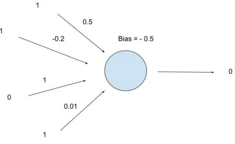
Each perceptron in a network has a correspondingbiasthat is added to the output of that perceptron before the output gets passed as input to the next layer. If the sum of all the weighted inputs into a perceptron plus the bias of that perceptron is greater than or equal to 0, then that perceptron will output a 1. Otherwise, that perceptron will output a 0. As a result of this, the negative bias of a perceptron is sometimes referred to as the threshold. Figure 2.2 shows an example of a perceptron with four inputs where the output is 0. This is because
[1(0.5)+1(−0.2)+0(1)+1(0.01)] −0.5−0.19 <0.
When we bring the concepts of both weights and biases together, it gives us the ability to start thinking about how to tune a neural network to help us make decisions.
Sigmoid Neurons 5
2.2
Sigmoid Neurons
The main problem with perceptrons is that making subtle changes to the weights and biases can sometimes result in massive changes to the output, which is not ideal. For example, let’s build a network with 3 input perceptrons and 1 output perceptron. The starting weights and the bias of the output perceptron can be initialized randomly. Figure 2.3 shows that the output of this neural network is 1 for the input 1,0,1. This is because
[1(0.9)+0(0.4)+1(−0.5)]+(−0.4)0≥0.
Figure 2.3 Neural network built with perceptrons.
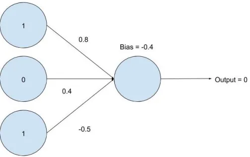
Let’s now consider this same network, but with slightly different weights. Let’s change the weight of the edge from the topmost input perceptron to the output perceptron from 0.9 to 0.8 in Figure 2.4. With the same input of 1,0,1, the network now outputs 0. This is because
6 What is a Neural Network?
Figure 2.4 A slight change in weights in perceptron network results in a differ-ent output.
Subtle changes in the network’s weights and biases should ideally result in subtle changes in the network’s output, allowing the network’s weights and biases to be tuned. The second type of artificial neuron, the sigmoid neuron, has this property.
Thesigmoid neuron is the main neuron model that is used today in neural networks. Its function is similar to that of perceptrons, but when there are subtle changes to the weights and biases, there are not massive changes to the output. The inputs to a sigmoid neuron can be anywhere between 0 and 1, and the output is determined by the weights of the inputs and the bias along with the sigmoid functionσ, where
σ(z) ≡ 1 1+e−z.
This sigmoid function is what prevents massive changes in the output when the network is tuned. This is because
lim x→−∞σ (z)0 and lim x→∞σ (z)1.
Sigmoid Neurons 7
This means that a sigmoid neuron’s output will always be contained in[0,1]. Let’s consider the two networks built with perceptrons in Figure 2.3 and Figure 2.4, but let’s use sigmoid neurons in the networks instead of perceptrons. Using the same weights and bias as in Figure 2.3, this sigmoid neuron network in Figure 2.5 outputs 0.5 with the input 1,0,1. This is because
σ([1(0.9)+0(0.4)+1(−0.5)]+(−0.4))σ(0) 1
1+e−0 0.5.
Figure 2.5 Neural network built with sigmoid neurons.
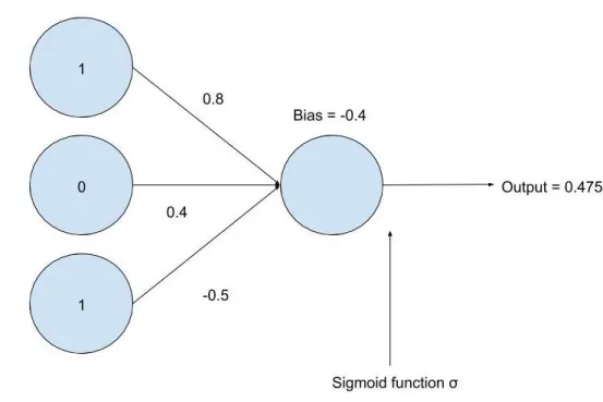
Changing the weights in the same way as in Figure 2.4 gives us a new network in Figure 2.6. This network outputs 0.475 with the input 1,0,1. This is because
σ([1(0.8)+0(0.4)+1(−0.5)]+(−0.4))σ(−0.1) 1
1+e0.1 0.475.
This shows that a subtle change in the weights of a sigmoid neuron network resulted in a subtle change in its output.
8 What is a Neural Network?
Figure 2.6 A slight change in weights in sigmoid neuron network results in a similar output.
The sigmoid function is an example of an activation function. An
activation functionis a function applied to the outputs of a layer in a neural network to introduce nonlinearities before this output is used as input in the next layer. Without activation functions, a neural network would just be one large affine transformation. In the context of activation functions, biases are used to shift an activation function left or right depending on at what inputs the activation function is triggered. For example, one popular activation function is theReLU function, defined as
f(x)max(0,x). Consider the networks in Figure 2.7 and Figure 2.8.
Sigmoid Neurons 9
Figure 2.7 An input that fails to trigger the activation function of a network.
In Figure 2.7, the network computes
ReLU([1(0.5)+0(0.4)+1(−0.5)]+1)ReLU(1)1.
In this case, the ReLU function wasn’t really used since ReLU(1)1. This is the same output the network would’ve given if there was no activation function on the output neuron at all.
10 What is a Neural Network?
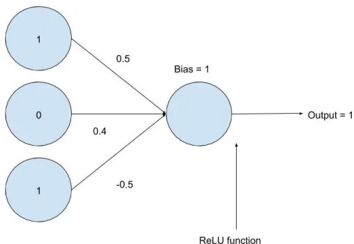
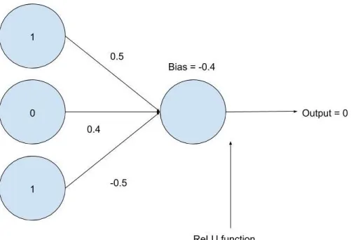
Figure 2.8 An input that triggers the activation function of a network.
In Figure 2.8, the network computes
ReLU([1(0.5)+0(0.4)+1(−0.5)]+(−0.4))ReLU(−0.4)0.
In this case, the Relu function is used since ReLU(−0.4) , −0.4. This is different from the output the network would’ve given if there was no activation function on the output neuron at all. Thus, changing the bias shifted the activation function to the right, allowing it to have an impact on the output of the network.
2.3
A Simple Model for Decision Making
The same process used to change the weights and biases of a perceptron network is also used for a sigmoid network. However, for the sake of simplicity, this section will demonstrate how a neural network made of perceptrons changes its weights and biases. The mathematics behind this will be discussed more in Section 2.5.
Let’s build a network that models the majority function (10). If the majority of inputs are 1, the correct output is 1. If the majority of inputs
A Simple Model for Decision Making 11
are 0, the correct output is 0. This network has 3 input perceptrons and 1 output perceptron. Let’s say we randomize the network’s weights and the output perceptron’s bias. Figure 2.9 shows a diagram of this network. With an input of 1,0,1, the network computes
[1(−0.5)+0(.4)+1(−0.5)]+(0)−1<0.
The network then outputs 0, which is incorrect in this case. The correct answer was 1, giving an error of 2.
Figure 2.9 Modeling the majority function with a perceptron neural network.
This error of 2 now gets split up between the perceptron weights that contributed to the network’s output. Because the input perceptron with an input of 0 didn’t contribute to the output at all, only two of the weights change. Figure 2.10 shows the result of adding 1 to each of the weights of the two perceptrons that contribute to the output.
12 What is a Neural Network?
Figure 2.10 Adjusting the weights of a neural network.
After adjusting these weights, with the same input of 1,0,1, the network compute
1(0.5)+0(0.4)+1(0.5)1≥0. This gives an output of 1, which is correct for this input.
2.4
Layers
The overall architecture of a neural network includes 3 main types of layers. The first layer of a neural network is known as theinput layerand is where the input data is recorded. The dimension of the instance of input data corresponds to the number of input neurons in the network. For example, if the data is a set of 5 by 5 matrices, then there will be 25 input neurons, each encoding a number in our matrix.
The second type of layer is called ahidden layer. There can be multiple hidden layers in a neural network, and the number of neurons in each layer is something to be experimented with depending on what the neural network is built to accomplish.
Theoutput layeris the final type of layer. If the network needs to have 3 outputs, each with its own meaning, there should be 3 different output
Gradient Descent and Learning 13
neurons, one for each output.
Some machine learners have different terms for different types of neural networks. One of the most common terms isdeep neural network. A deep neural network has a certain number of hidden layers. This number has changed over time as computation has improved. Currently, a deep neural network might contain at least 5-10 hidden layers. Afeedforward neural network is a network that only passes outputs from individual neurons forward from the input layer to the output layer. Afully connected neural networkis a network in which there is a weighted edge passing output from every neuron in a given layer to every neuron in the next layer as input. The neural networks built and used for this thesis are all feedforward networks that are fully connected. Figure 2.11 is an example of a small feedforward, fully connected network.
Figure 2.11 Feedforward, fully connected neural network.
2.5
Gradient Descent and Learning
Learning algorithmsare the method by which a network can tune its weights and biases according to training data. Training datais a set of data that is run through a neural network repeatedly to adjust the network’s weights and biases. After running a particular data instance through a network, the network adjusts its weights and biases based on how far away its output is from the correct output.
14 What is a Neural Network?
its weights and biases in an optimal way for a particular type of input and output. Two different data sets are used when learning with gradient descent. The first is a training data set, which will be inputted into the network multiple times in order to adjust the network’s weights and biases. The second is the validation set. Thevalidation settests the neural network’s knowledge after it is trained. The general rule of thumb if there is a limited amount of data to work with is sometimes known as the "80/20 Rule". The rule is to split the data so that 80% is training data and 20% is validation data.
When training a network using gradient descent, let y(x)be the desired output. Gradient descent uses a loss function to comparey(x)top(x), the network’s actual output. Aloss functionis a function that describes how far the network’s actual output is from the expected or desired output.
Let’s define a loss function,L, that gradient descent will try to minimize:
L(w,b) ≡ 1 2n Õ x | |y(x) −a(x)| |2 where
• wis the set of weights in the network
• bis the set of biases
• nis the total number of training inputs
• a(x)is the vector of outputs from the network whenxis the input
• y(x)is the correct or desired output from the network whenxis the input
• xis a particular training input.
The value of the loss functionLshould ideally be as small as possible since it represents the difference between the neural network’s actual output and desired output. In order to find this minimum, the algorithm needs to make small changes inwandb, denoted∆wand∆b. These small changes
∆wand∆bcorrespond to∆L, the small change inL:
∆L ≈ ∂L
∂w∆w+
∂L
Gradient Descent and Learning 15
Notice that∇L, the gradient ofL, is
∇L≡ (∂L
∂w,
∂L
∂b)
T.
Rewriting∆Lusing∇Lyields
∆L≈ ∇L·∆v
where v [w,b]. Gradient descent is a way of taking small steps in the direction which does the most to immediately decreaseL, so∆Lshould be negative. In order to make∆Lnegative, the learning algorithm needs to choose∆wand∆baccordingly. Let’s choose
∆v−η∇L
whereηis small and positive. The parameterηis known as thelearning rateand represents the size of the step the algorithm takes during gradient descent. This equation is then used to repeatedly computeveach time the algorithm takes a new step towards the minimum ofLsuch that
∆vvf −vi η∇L.
Because learning requires the computation of many derivatives, it can sometimes be a slow process. Stochastic gradient descentis meant to be a quicker version of gradient descent because instead of calculating ∇L for all of the training inputs, in stochastic gradient descent, the algorithm just calculates∇Lfor a small sample of randomly chosen inputs. This greatly improves the speed of the gradient descent since it is no longer necessary to calculate∇Lfor every data instance in the training set.
There are many different types of loss functions used throughout machine learning, but the one I use in my binary classification neural networks is called a binary cross entropy function. Abinary cross entropy function
is a function that measures the performance of a model whose output is a probability value between 0 and 1. A binary cross entropy function B(x,y(x),a(x))can be written as
B(x,y(x),a(x))−[y(x)log(p(x))+(1−y(x))log(1−p(x))] where
16 What is a Neural Network?
• y(x)is the correct or desired output from the network whenxis the input
• p(x)is the predicted probability of that classification.
A binary cross entropy function is also sometimes referred to as alog loss function. Figure 2.12 shows the log loss function when y(x)1 for a particular inputx, meaning the correct labeling of an inputxis 1. If a neural network predicts a label of 0, the log loss function in Figure 2.12 gives a large loss. This is desirable since 0 was not the correct labeling. If a neural network predicts a label of 1, the log loss function in Figure 2.12 gives a small loss. Again, this is desirable since 1 is the correct labeling.
Chapter 3
Generating Data
3.1
Training and Validation Data
I used MATLAB (11) to generate large amounts of data for training and validation of the neural networks I created for this thesis. Each of the training sets and validation sets I generated contained 20,000 data instances. I then took the csv files outputted by my MATLAB code and used a Python (12) package called Pandas (13) to create data structures called dataframes, which are essentially large matrices with labels.
Since I am considering data on a circle, it is useful to consider binning the data so that there is a finite number of points on the circle. In this case, I always generated data instances with a total of 128 total points. I did this by having my MATLAB code pick a bin on the circle according to some probability distribution and then increase that bin value by 1. I would then repeat this process 128 times, where 128 is the total number of points on the circle.
I generated data for the uniform distribution, the von Mises distribution, the semicircular distribution (where each half of the circle has a different probability), and the linear distribution (where the probability of picking a bin increases linearly around the circle) using 128 bins on the circle. I chose 128 purely because it is a power of 2. In addition, for each data instance I generated, I chose a random number between 1 and 128 and rotated the data instance that number of bins so that every data instance wouldn’t have a high number of points in the same general area. Failing to do this would have made it easier for a neural network to distinguish between uniform and nonuniform distributions.
18 Generating Data
3.2
Uniform Distribution
In generating the uniform distribution, each bin has an equal probability of being chosen, meaning fornbins each bin has probability n1 of being chosen. In this case, since there are 128 bins, each bin has probability1281 of being chosen. Figure 3.1 shows an example of a sample of points coming from uniform distribution on a circle.
Figure 3.1 Example of a sample of points coming from a uniform distribution of circular data.
3.3
Linear Distribution
To understand the linear distribution on circular data, imagine a line of slope mwrapped around a circle. Figure 3.2 shows an example of a sample of points coming from a linear distribution on a circle.
Figure 3.2 Example of a sample of points coming from a linear distribution of circular data.
In order to generate this data, I randomly chose a slopembetween 0.1 and 0.2. This range of slopes was chosen because the values are small and
von Mises Distribution 19
can work for circles that don’t have a large number of points, but the values are not so big that it visually gives away the fact there is a linear distribution on the circle. Then, in order to randomly sample from the distribution to choose bins, I calculated the area, A, under a line with slope m and x-length equivalent to the number of bins on our circlen, in this case 128, by calculating
A 1
2 ·n· (m·n).
Then I calculated the area, Y, under a line with slope m and x-length equivalent to a number,x, between 1 andnby calculating
Y 1
2 ·x· (m·x).
Thus, the probability of choosing thexth bin or less is P(X≤ x) Y
A x2
1282.
I found the probability of choosing thexth bin exactly using P(Xx) Y − (1 2 · (x−1) · (m· (x−1))) A 2x−1 2 A 2x−1 mn2 .
3.4
von Mises Distribution
The von Mises distribution is a type of unimodal distribution on circular data controlled by two parametersµandκ. The parameterµcontrols the location of where the majority of the points are concentrated on the circle, and the parameterκis a measure of how concentrated the points are around the chosen location. Figure 3.3 shows an example of a sample of points coming from a unimodal distribution on a circle.
Figure 3.3 Example of a sample of points coming from a unimodal distribution of circular data.
20 Generating Data
The probability density function for the von Mises distribution for an anglexranging between 0 and 2πis given by
f(x|µ, κ) eκ
cos(x−µ)
2πI0(κ)
whereI0(κ)is the modified Bessel function of order 0 (5). Figure 3.4 shows
the von Mises probability distribution for a range ofκvalues.
Figure 3.4 von Mises probability density function for a range ofκvalues (5).
When generating von Mises distributions, I did not take into account the denominator of the probability density function since it is only used for scaling.
3.5
Semicircular Distribution
To generate data coming from the semicircular distribution, it is useful to think about having two uniform distributions, one on some half of the circle and one on the other. One of these uniform distributions is sampled with higher probability than the other. Figure 3.5 shows an example of a sample of points coming from a semicircular distribution on a circle. The top portion of the circle has a uniform distribution that is being sampled with higher probability than the bottom portion.
Duplicates 21
Figure 3.5 Example of a sample of points coming from a semicircular distri-bution on circular data.
3.6
Duplicates
After generating data for the training set, I generated data for the validation set. In doing so, I noticed that there were occasionally duplicate data instances between the two sets. At first, this seemed like a bad thing. In many online examples of neural networks, this would be undesirable, especially if a network was doing something like image processing. It is not desirable to train a network on a particular image multiple times, meaning a particular instance or image is in the training set more than once. This would bias the network towards that image. However, in the context of classifying probability distributions on a circle, having duplicates in the training data and validation data makes sense as long as they are generated by different distributions.
Figure 3.6 Two similar data instances sampled from different distributions.
The two data instances in Figure 3.6 are extremely similar and could both be classified as uniform. However, they could each also be classified
22 Generating Data
as instances of the semicircular distribution with each half of the circle having an almost equal probability. Thus, because a given data instance can be generated using multiple distributions, the network needs to take into account those that are more likely to occur (i.e. generated more frequently). Because some data instances can be classified in multiple ways, the network needs to learn for itself that it shouldn’t be too certain about its classification of one of these frequently generated data instances.
Chapter 4
Tests for Uniformity
4.1
Beran’s Test for Uniformity
In his 1968 and 1969 papers (6; 7), Beran constructs a test statistic for discrete circular data to test for uniformity that implicitly uses Fourier coefficients of the data. I will use this section to outline his test statistic.
Let’s view an instance of discrete circular data as a function on the cyclic groupGZ/NZwhere the bins on the circle correspond to group elements. Let f, another function on this same cyclic group, be some nonuniform alternative density where Í
g∈G f(g) |G| N. Consider the following
statistic Tn 1 nN Õ g∈G [ n Õ i1 f(g gi) −N]2 where
• nis the total number of data points in the data instance
• Nis the dimension of the data instance
• Gis the cyclic group onNelements
• g gi is the data instance on theith group element moved by another
group element g.
24 Tests for Uniformity
Figure 4.1 Function on the cyclic group onNelements.
Let’s writeaas a vector
a a0 a1 ... an−1 .
The function on the 0th element, ¯0, isa0. The function on the 1st element, ¯1,
isa1and so on.
Figure 4.2 Before and after rotating by a group element.
Figure 4.2 shows the before and after of rotatingaby one bin on the circle whena1 4.This is equivalent to a group element acting ona, causinga to
shift on the circle. Theg gi term in Beran’s statistic represents shifting the
group elementgi by a group action using g ∈ Gand enables the statistic
to take into account rotated versions ofa. This is how Beran accounts for the rotational symmetry of a circle in his statistic. TheÍni1 f(g gi)term represents taking the inner product of the alternative density f with one rotated version of the data instanceato get a measure of how similar f and
Beran’s Test for Uniformity 25
that version ofaare. The−Npart of Beran’s statistic represents removing the pieces of both f andathat contribute to the uniform distribution. Essentially, Beran’s statistic considers the pieces of f andathat are orthogonal to the all-ones density and then uses inner products to compare how similar this piece of f is to all the rotated versions of this piece ofa. He measures how similar they are by summing up all of the squares.
Cross correlationis exactly the idea of taking an inner product of one function with a shifted version of another function. In fact, because f anda in this context are both real-valued, cross correlation can be computed using convolution, and the convolution of two functions in the time domain is just the product of their Fourier transforms in the frequency domain. This means that in his statistic, Beran is usingFourier coefficientsof the data instance and the alternative density (7).
Chapter 5
Creating the Network
5.1
Initial Network Structure
When I was learning how to actually code up a neural network, I started with a very small network. It had the same structure as the network in Figure 5.1.
Figure 5.1 Initial neural network structure.
This network has 8 input neurons, 1 hidden layer with 8 neurons, and 1 output neuron. Each neuron in a particular layer is connected to every
28 Creating the Network
neuron in the next layer, making this network fully-connected. This network is also feedforward.
Training Epoch Loss
0 0.4598 1 0.4886 2 0.5058 3 0.5149 4 0.5186 5 0.5189 6 0.5168 7 0.5134 8 0.5090 9 0.4989 10 0.4935 11 0.4880 12 0.4825 13 0.4768 14 0.4768 15 0.4712 16 0.4657 17 0.4601 18 0.4546 19 0.4492
Mimicking Beran’s Test 29
Figure 5.2 Training loss of a small neural network.
Table 5.1 and Figure 5.2 show that while the loss of this small network does decrease after 20 training epochs, it decreases only a small amount and increases a good amount in the middle of training. This sort of output is not ideal and signals that a larger network is needed to get better results.
5.2
Mimicking Beran’s Test
Remember Beran’s statistic (6; 7) is
Tn 1 nN Õ g∈G [ n Õ i1 f(g gi) −N]2 where
• nis the total number of data points in the data instance
• Nis the dimension of the data instance
• Gis the cyclic group onNelements
• g gi is the data instance on theith group element moved by another
30 Creating the Network
Let an example input vector be
a 3 5 9 7
such thatn 24 andN4. Let our alternative density f be the semicircular distribution with probability 0.33 on one semicircle and probability 0.67 on the other semicircle. Remember that since this is a density all of the entires in f must sum toN. f 2 3 2 3 4 3 4 3 .
We can compute the inner portion of the statistic, meaning theÍ
g∈GÍni1 f(g gi)
portion, very easily with a simple neural network in Figure 5.3.
Network Structure 31
In terms of squaring the outputs from the hidden layer like Beran does in his statistic, there is the possibility of using a special activation function between layers. However, squaring doesn’t seem to be an activation function that is commonly used among the neural network community. However, the ReLU function is quite commonly used. Since the ReLU function is 0 when the input is less than 0 and is equal to the value of the input otherwise, it almost acts as an absolute value. While the ReLU function does not have the same utility as squaring the input, for the purposes of trying to measure the largeness of something, taking something similar to the absolute value has meaning.
The main problem with this network once it was created and tested was that it was too small both in the number of nodes in all of the non-output layers and in the number of layers itself, meaning it didn’t do a great job of classifying the inputted probability distributions.
While a such a small neural network was not powerful enough to compute Beran’s statistic, it is known that a neural network can approximate Beran’s statistic arbitrarily well (14).
5.3
Network Structure
In playing around with network size, I tried a much larger network of 5 layers. However, when training this network, the network was able to reach 100% training accuracy way too quickly while the validation accuracy was still quite low, signaling the network was big enough to memorize the inputs and outputs in the data. Eventually, I found that a network with 1 input layer, 1 smaller hidden layer, and 1 output layer is able to differentiate between uniform and nonuniform probability distributions on circular data quite well.
Below, I provide some snippets of code in Python (12) used to construct the neural networks used for this thesis. There are many different Python libraries people like to take advantage of when trying to build neural networks. This thesis uses PyTorch (15) and Pandas (13).
After importing the necessary tools and importing the data as Pandas dataframes, I separated the training data from the validation data. Note that
datais the name of the Pandas dataframe containing the training data and
valis the name of the Pandas dataframe containing our validation data.
Because I generated my own data, I was not restricted to the 80/20 rule and had training sets and validation sets of equal size. Both the training set and
32 Creating the Network
validation set contained 20,000 data instances each.
f = data.as_matrix(columns=[List of Column Names]) g = val.as_matrix(columns=[List of Column Names])
After separating out the validation set from the training set, I separated the labels for a data instance as to whether it is uniform or nonuniform from the data instances themselves. In this case, these answers are contained in a column denoted with the nameU.
x_train = torch.Tensor(f)
y_train = torch.Tensor(data.as_matrix(columns=[’U’])) x_val = torch.Tensor(g)
y_val = torch.Tensor(val.as_matrix(columns=[’U’]))
Then I created a TensorDataset, which I used to load the data and split into groups. Each of these groups is called abatch. Each batch is run through the network once during each period of training and validation, called an
epoch. Over one epoch, the whole training data set and validation data set will have been run through the network once in batches.
train_ds = TensorDataset(x_train, y_train)
train_dl = DataLoader(train_ds, batch_size=1024, shuffle=True) val_ds = TensorDataset(x_val, y_val)
val_dl = DataLoader(val_ds, batch_size=1024, shuffle=True) #batch size: how many samples per batch to load (default: 1)
After creating the TensorDataset, I named and created the model and set the learning rate. This learning rate has to do with how large of a step is taken during gradient descent.
def get_model():
model = UniformPredictor()
return model, optim.SGD(model.parameters(), lr=0.01)
Here the input layer has 128 neurons, the hidden layer has 4 neurons, and the output layer has 1 neuron.
class UniformPredictor(nn.Module): def __init__(self):
super().__init__()
Network Structure 33 self.fc2 = nn.Linear(4,1) self.m = torch.nn.Sigmoid() def forward(self, xb): return self.m(self.fc2(F.relu(self.fc1(xb)))) model,opt = get_model()
The training loop loops over the training data 10 times sinceepochs = 10. Within this loop, the model is trained on sets of data instances that are of the chosen batch size set above. This means the model makes a prediction using an instance of training data, measures how well that prediction matches the correct answer, and adjusts its weights and biases accordingly.
epochs = 10
loss_func = F.binary_cross_entropy for epoch in range(epochs):
#train
for xb,yb in train_dl: pred = model(xb)
loss = loss_func(pred, yb) loss.backward()
opt.step() opt.zero_grad()
Here is the validation loop. Note that here the model makes a prediction and then later compares that to the correct answer. However, the model does not adjust its weights and biases at all based on these predictions.
for epoch in range(epochs): for xv,yv in val_dl:
Chapter 6
Results
In this section, I share the results of running the Rayleigh Test (1), the Watson Test (2), and the Ajne Test (3) on discrete circular data instances sampled from uniform and nonuniform distributions, and I also describe the results of training and validating neural networks to differentiate between these same data instances. These data instances each contain 128 data points distributed over 128 bins based on which distribution is being sampled. In addition to comparing the accuracy, type I error, and type II error of this set of statistical tests and the networks trained on data instances without any preprocessing, I also compare the effects of training and validating networks on preprocessed data.
6.1
Running Statistical Tests on Data Instances
Sam-ple from Uniform and Nonuniform Distributions
This section contains the results of running the Rayleigh Test (1), the Watson Test (2), and the Ajne Test (3) on discrete circular data instances sampled from uniform and nonuniform distributions. In running these three tests, I empirically calculated p-values by comparing test statistics obtained by running the training and validation data of the networks I created through this set of statistical tests with the test statistics for a separate group of data instances sampled from a uniform distribution. Because I calculated p-values empirically, I needed to choose a significance level for each test. I did so by calculating accuracy using a wide range of significance levels and then picked the significance level for which a test had the highest accuracy. Atype I erroris when the null hypothesis is incorrectly rejected. In
36 Results
this case, the null hypothesis is that a data instance is being sampled from a uniform distribution, so a type I error is when a data instance sampled from a uniform distribution is incorrectly classified as being sampled from a nonuniform distribution. Atype II erroris when the null hypothesis is incorrectly not rejected. In this case, a type II error is when a data instance being sampled from a nonuniform distribution is incorrectly classified as being sampled from a uniform distribution.
Beran identifies the alternative density in the Rayleigh Test (1) as the unimodal distribution. Table 6.1 shows the accuracy percentage, type I error as percentage of total error, and type II error as a percentage of total error from running 20,000 data instances sampled from a uniform distribution and 20,000 data instances sampled from the von Mises distribution through the Rayleigh Test (1) using a confidence level of 0.01. The von Mises distribution is a type of unimodal distribution.
von Mises and uniform distribution through Rayleigh w/ 0.01 confidence level
Correct% 99.6% Type I Error as % of all Error 100% Type II Error as % of all Error 0%
Table 6.1 von Mises and uniform distribution through Rayleigh w/ 0.01 confi-dence level.
Beran identifies the alternative density in the Watson Test (2) as the linear distribution. Table 6.2 shows the accuracy percentage, type I error as percentage of total error, and type II error as a percentage of total error from running 20,000 data instances sampled from a uniform distribution and 20,000 data instances sampled from a linear distribution with a randomly chosen slope ranging from 0.1 to 0.2 through the Watson Test (2) using a confidence level of 0.1.
Running Statistical Tests on Data Instances Sample from Uniform and Nonuniform Distributions 37
Linear and uniform distribution through Watson w/ 0.01 confidence level
Correct% 99.5% Type I Error as % of all Error 91.4% Type II Error as % of all Error 8.6%
Table 6.2 Linear and uniform distribution through Watson w/ 0.01 confidence level
Beran identifies the alternative density in the Ajne Test (3) as the semicir-cular distribution. Table 6.3 shows the accuracy percentage, type I error as percentage of total error, and type II error as a percentage of total error from running 20,000 data instances sampled from a uniform distribution and 20,000 data instances sampled from the semicircular distribution through the Ajne Test (3) using a confidence level of 0.03. This semicircular distribution has a random number of points uniformly distributed on a randomly chosen half of the circle and then has 128 minus the random number of points on the chosen first half uniformly distributed on the remaining second half.
Semicircular and uniform distribution through Ajne w/ 0.03 confidence level
Correct% 86.82% Type I Error as % of all Error 10.8% Type II Error as % of all Error 89.2%
Table 6.3 Semicircular and uniform distribution through Ajne w/ 0.03 confi-dence level.
Table 6.4 contains the accuracy percentage, type I error as percentage of total error, and type II error as a percentage of total error from running 20,000 data instances sampled from a uniform distribution and 20,000 data instances sampled from a nonuniform distribution through a set of statistical tests for uniformity. Each test in the table was run on the data instances sampled from the nonuniform distributions that come from the corresponding alternative densities. Table 6.4 shows that the Rayleigh Test (1) had the best accuracy out of all the tests shown.
38 Results
Test Confidence Level Correct% Type I Error Type II Error Ajne 0.03 86.82% 10.76% 89.24% Watson 0.01 99.5% 91.4% 8.6% Rayleigh 0.01 99.57% 100% 0%
Table 6.4 Summary of statistical test results.
6.2
Training and Validating Neural Networks on Data
Without Preprocessing
In this section, I give results for the accuracy, type I, and type II errors for training and validating specific neural networks trained on data instances that were not preprocessed.
6.2.1 Network Trained to Compete with the Rayleigh Test
In this section, I discuss the results from training and validating a neural network to distinguish between data instances sampled from a uniform distribution and data instances sampled from the von Mises distribution. Even with very little training time, this network was able to achieve an extremely high accuracy and was able to outperform the Rayleigh Test (1).
Training and Validating Neural Networks on Data Without Preprocessing 39
The validation accuracy rose very quickly to 100% in Figure 6.1, and the loss dropped very quickly in Figure 6.2.
Figure 6.2 Loss for von Mises and uniform distribution classifier.
In addition, since the accuracy rose so quickly, the type I and type II error dropped very quickly to 0 in Figure 6.3.
40 Results
There are many reasons why this network might have been able to do so well. One worth noting is that even to the human eye, a unimodal distribution is easier to pick out from a group of uniform distributions since the majority of points are concentrated in one region on the circle. Remember that the Rayleigh test was able to achieve 99.6% accuracy, but this network was able to achieve 100% validation accuracy. Table 6.5 gives an accuracy comparison between the Rayleigh Test (1) and this network.
Rayleigh Test Network 99.6% 100%
Table 6.5 Accuracy comparison of the Rayleigh test and the network trained on von Mises and uniform distributions
6.2.2 Network Trained to Compete with the Watson Test
In this section, I discuss the results from training and validating a neural network to distinguish between data instances sampled from a uniform distribution and data instances sampled from the linear distribution. While this network was trained for a much longer training period of 200 training epochs as opposed to the 70 epoch training period for the network in Section 6.2.1, most of the increase in accuracy happens within the first 60 epochs in Figure 6.4.
Training and Validating Neural Networks on Data Without Preprocessing 41
Figure 6.4 Accuracy for linear and uniform distribution classifier.
This network was able to achieve a validation accuracy of 98.9%, which is slightly lower than the Watson Test’s (2) accuracy of 99.5%. In Figure 6.5, the loss drops slightly slower than the accuracy rises in Figure 6.4.
42 Results
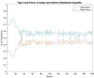
Figure 6.6 shows the type I and type II error as a fraction of the total error. This is interesting in comparison to Table 6.2. Most of the Watson Test’s (2) and this network’s errors are coming from type I errors, meaning they are more likely to incorrectly classify a uniform distribution as a nonuniform distribution.
Figure 6.6 Type I and II error for linear and uniform distribution classifier.
Table 6.6 gives an accuracy comparison between the Watson Test (2) and this network.
Watson Test Network 99.5% 98.9%
Table 6.6 Accuracy comparison of the Watson test and the network trained on linear and uniform distributions
6.2.3 Network Trained to Compete with the Ajne Test
In this section, I discuss the results from training and validating a neural network to distinguish between data instances sampled from a uniform distribution and data instances sampled from the semicircular distribution. Similarly to the network in Section 6.2.2, this network also trained for a
Training and Validating Neural Networks on Data Without Preprocessing 43
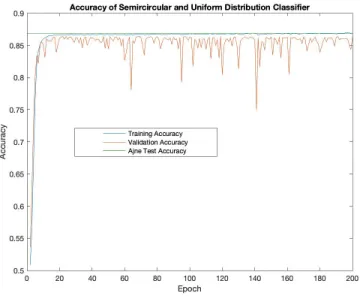
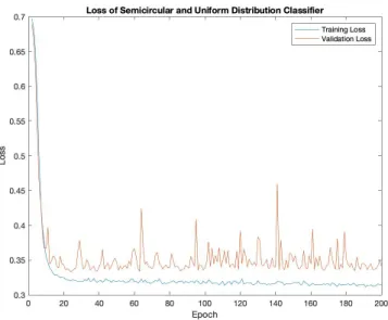
longer training period, but most of the increase in accuracy happened within the first 20 training epochs in Figure 6.7. Both Figure 6.7 and Figure 6.8 show that the validation accuracy and loss respectively have a fairly large variance over the training period. This suggests that while the validation accuracy and loss is tracking the training accuracy and loss (which signals the network has learned to pick up on features in the data), it can still be quite difficult for the network to classify instances it hasn’t seen before.
44 Results
Figure 6.8 Loss for semicircular and uniform distribution classifier.
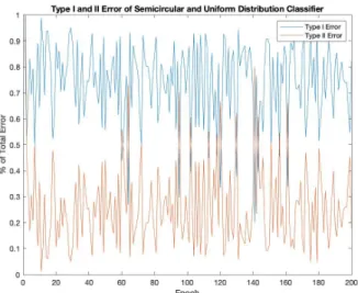
Like the network in Section 6.2.2, this network tends to make more type I errors than type II errors in Figure 6.9. Remember that the Ajne test (3) only had 10.8% of its error coming from type I error, meaning that majority was type II error. This means that this network is most likely to incorrectly classify a data instance being sampled from a uniform distribution as being sampled from a nonuniform distribution whereas the competing statistical test is more likely to incorrectly classify a data instance being sampled from a nonuniform distribution as being sampled from a uniform distribution.
Data Preprocessing: Discrete Cosine Transform 45
Figure 6.9 Type I and II error for semicircular and uniform distribution classi-fier.
Table 6.7 gives an accuracy comparison between the Ajne Test (3) and this network.
Ajne Test Network 86.8% 86.5%
Table 6.7 Accuracy comparison of the Ajne test and the network trained on semicircular and uniform distributions
6.3
Data Preprocessing: Discrete Cosine Transform
In this section, I give results for the accuracy, type I, and type II errors for training and validating specific neural networks trained on data instances that were preprocessed with the discrete cosine transform. Preprocessing in general can often results in shorter training times or better accuracy results since it picks out distinguishing characteristics of the data for the network instead of the network trying to pick these itself. The discrete cosine
46 Results transform is y(k) r 2 N−1 N Õ n1 x(n)√ 1 1+δk1+δkNcos ( π N−1(n−1)(k−1)) where
• Nis the length of a signalx
• kgoes from 1 toN
• δkiis the Kronecker delta(16).
The DCT is often used in similar contexts where a Fourier transform might be used. This is because the Fourier transform is a projection onto the space spanned by cosines and sines, a complex-valued space. However, since the DCT is a projection only onto the cosines, the outputs of the DCT are all real-valued.
6.3.1 DCT for Network Trained to Compete with the Rayleigh Test
In this section, I discuss the results from training and validating a neural network to distinguish between data instances sampled from a uniform dis-tribution and data instances sampled from the von Mises disdis-tribution. Before passing a data instance as input to the network, the data was preprocessed with the discrete cosine transform.
Data Preprocessing: Discrete Cosine Transform 47
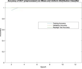
Figure 6.10 Accuracy for DCT preprocessed von Mises and uniform distribu-tion classifier.
Figure 6.10 shows that a network trained and validated with instances sampled from the von Mises and uniform distributions can perform really well. Preprocessing the data in this case with the DCT did not seem to impact the results of this network. The validation accuracy reaches 100% as it did in the network trained on data that was not preprocessed, and overall this network does better than the 99.6% accuracy achieved by the Rayleigh test (1).
48 Results
Figure 6.11 Loss for DCT preprocessed von Mises and uniform distribution classifier.
Figure 6.11 shows the loss of this network during training and validation dropping very quickly, and Figure 6.12 shows the error dropping very quickly as well.
Data Preprocessing: Discrete Cosine Transform 49
Figure 6.12 Type I and II error for DCT preprocessed von Mises and uniform distribution classifier.
Table 6.8 gives an accuracy comparison between the Rayleigh Test (1) and two networks trained and validated with data instances, not preprocessed and preprocessed with the DCT, sampled from the uniform distribution and the von Mises distribution.
Rayleigh Test No preprocessing DCT 99.6% 100% 100%
Table 6.8 Accuracy comparison of the Rayleigh test, no preprocessing, and DCT
6.3.2 DCT for Network Trained to Compete with the Watson Test
In this section, I discuss the results from training and validating a neural network to distinguish between data instances sampled from a uniform distribution and data instances sampled from the linear distribution. Before passing a data instance as input to the network, the data was preprocessed with the discrete cosine transform.
50 Results
This network was able to achieve a validation accuracy of 98.7% in Figure 6.13. This is slightly lower than the 98.9% accuracy that the network trained on linear and uniform distributions that were not preprocessed was able to achieve in Figure 6.4. This network also failed to beat the Watson test’s (2) 99.5% accuracy in Table 6.2.
Figure 6.13 Accuracy for DCT preprocessed linear and uniform distribution classifier.
Figure 6.14 shows that the loss for this network doesn’t drop as quickly as the accuracy rises in Figure 6.13.
Data Preprocessing: Discrete Cosine Transform 51
Figure 6.14 Loss for DCT preprocessed linear and uniform distribution classi-fier.
Figure 6.15 shows that while this network is similar to the one trained on the nonpreprocessed data in that it is most likely to make a type I error, they are different in that this network’s type I and type II error fractions are much closer.
Figure 6.15 Type I and II error for DCT preprocessed linear and uniform distri-bution classifier.
52 Results
Table 6.9 gives an accuracy comparison between the Watson Test (2) and two networks trained and validated with data instances, not preprocessed and preprocessed with the DCT, sampled from the uniform distribution and the linear distribution.
Watson Test No preprocessing DCT 99.5% 98.9% 98.7%
Table 6.9 Accuracy comparison of the Watson test, no preprocessing, DCT
6.3.3 DCT for Network Trained to Compete with the Ajne Test
In this section, I discuss the results from training and validating a neural network to distinguish between data instances sampled from a uniform distribution and data instances sampled from the semicircular distribu-tion. Before passing a data instance as input to the network, the data was preprocessed with the discrete cosine transform.
Figure 6.16 Accuracy for DCT preprocessed semicircular and uniform distri-bution classifier.
Data Preprocessing: Discrete Cosine Transform 53
beat the Ajne test (3), but it achieved a comparable accuracy score. Figure 6.17 shows the loss for this network.
Figure 6.17 Loss for DCT preprocessed semicircular and uniform distribution classifier.
Figure 6.18 Type I and II error for DCT preprocessed semicircular and uniform distribution classifier.
54 Results
Figure 6.18 is similar to the error in Figure 6.9, with type I error making up the majority of the error.
Table 6.10 gives an accuracy comparison between the Ajne Test (3) and two networks trained and validated with data instances, not preprocessed and preprocessed with the DCT, sampled from the uniform distribution and the semicircular distribution.
Ajne Test No preprocessing DCT 86.8% 86.5% 86.1%
Table 6.10 Accuracy comparison of the Ajne test, no preprocessing, DCT
6.4
Data Preprocessing: Discrete Sine Transform
In this section, I give results for the accuracy, type I, and type II errors for training and validating specific neural networks trained on data instances that were preprocessed with the discrete sine transform. The discrete sine transform is y(k) N Õ n1 x(n)sin(π kn N+1) where
• Nis the number of bins on the circle
• k 1,· · · ,N.
The DST is often used in similar contexts where a Fourier transform might be used. This is because the Fourier transform is a projection onto the space spanned by cosines and sines, a complex-valued space. However, since the DST is a projection only onto the sines, the outputs of the DST are all real-valued.
6.4.1 DST for Network Trained to Compete with the Rayleigh Test
In this section, I discuss the results from training and validating a neural network to distinguish between data instances sampled from a uniform dis-tribution and data instances sampled from the von Mises disdis-tribution. Before
Data Preprocessing: Discrete Sine Transform 55
passing a data instance as input to the network, the data was preprocessed with the discrete sine transform.
Figure 6.19 Accuracy for DST preprocessed von Mises and uniform distribution classifier.
Figure 6.19 shows again that a network trained with data coming from the von Mises and uniform distribution can do really well in terms of accuracy. Preprocessing the data in this case with the DST did not seem to impact the results of this network. The validation accuracy reaches 100% as it did in the network trained on data that was not preprocessed, and overall this network does better than the 99.6% accuracy achieved by the Rayleigh test (1).
56 Results
Figure 6.20 Loss for DST preprocessed von Mises and uniform distribution classifier.
Figure 6.20 shows the loss drop very quickly, and Figure 6.21 shows the error dropping to 0 even more quickly.
Figure 6.21 Type I and II error for DST preprocessed von Mises and uniform distribution classifier.
Data Preprocessing: Discrete Sine Transform 57
Table 6.11 gives an accuracy comparison between the Rayleigh Test (1) and three networks trained and validated with data instances, not preprocessed and preprocessed with the DCT and DST, sampled from the uniform distribution and the von Mises distribution.
Rayleigh Test No preprocessing DCT DST 99.6% 100% 100% 100%
Table 6.11 Accuracy comparison of the Rayleigh test, no preprocessing, DCT, DST
6.4.2 DST for Network Trained to Compete with the Watson Test
In this section, I discuss the results from training and validating a neural network to distinguish between data instances sampled from a uniform distribution and data instances sampled from the linear distribution. Before passing a data instance as input to the network, the data was preprocessed with the discrete sine transform.
Figure 6.22 Accuracy for DST preprocessed linear and uniform distribution classifier.
58 Results
Using the DST instead of a DCT to preprocess the data produces two networks with almost the exact same accuracy, both of which are slightly lower than the accuracy for the network trained on nonpreprocessed data. All three networks fail to beat the accuracy of the Watson test (2), but they achieve comparable accuracy.
Figure 6.23 Loss for DST preprocessed linear and uniform distribution classi-fier.
Figure 6.24 shows much more overlap in type of error than Figure 6.6 or Figure 6.15, which is surpising because one might think that the type of error would be similar for two networks, one trained on data preprocessed with the DCT and one trained on data preprocessed with the DST.
Data Preprocessing: Discrete Sine Transform 59
Figure 6.24 Type I and II error for DST preprocessed linear and uniform distri-bution classifier.
Table 6.12 gives an accuracy comparison between the Watson Test (2) and three networks trained and validated with data instances, not prepro-cessed and preproprepro-cessed with the DCT and DST, sampled from the uniform distribution and the linear distribution.
Watson Test No preprocessing DCT DST 99.5% 98.9% 98.7% 98.6%
Table 6.12 Accuracy comparison of the Watson test, no preprocessing, DCT, DST
6.4.3 DST for Network Trained to Compete with the Ajne Test
In this section, I discuss the results from training and validating a neural network to distinguish between data instances sampled from a uniform distribution and data instances sampled from the semicircular distribu-tion. Before passing a data instance as input to the network, the data was preprocessed with the discrete sine transform.