A Behavioral Synthesis System for
Asynchronous Circuits
Matthew Sacker, Andrew D. Brown
, Senior Member, IEEE
, Andrew J. Rushton, and Peter R. Wilson
, Member, IEEE
Abstract—Behavioral synthesis of synchronous systems is a well established and researched area. The transformation of behavioral description into a datapath and control graph, and hence, to a structural realization usually requires three fundamental steps: 1) scheduling (the mapping of behavioral operations onto time slots); 2) allocation (the mapping of the behavioral operations onto abstract functional units); and 3) binding (the mapping of the functional units onto physical cells). Optimization is usually achieved by intelligent manipulation of these three steps in some way. Key to the operation of such a system is the (automatically generated) control graph, which is effectively a complex sequence generator controlling the passage of data through the system in time to some synchronizing clock. The maximum clock speed is dictated by the slowest time slot. (This is the timeslot containing the longest combinational logic delay.) Timeslots containing quicker (less) logic will effectively waste time: the output of the combinational logic in the state will have settled long before the registers reading the data are enabled. If we allow the state to change as soon as the data is ready, by introducing the concepts of “ready” and “acknowledge,” the control graph becomes a disjoint set of single-state machines—it effectively disappears, with the consequence that the timeslot–timeslot transitions become self controlling. Having removed the necessity for the timeslots to be of equal duration the system becomes selftiming: asynchronous. This paper describes a behavioral asynchronous synthesis system based on this concept that takes as input an algorithmic description of a design and produces an asynchronous structural implementation. Several example systems are synthesized both synchronously and asynchronously (with no modification to the high level de-scription). In keeping with the well-established observation that asynchronous systems operate at average case time complexity rather than worse case, the asynchronous structures usually operate some 30% faster than their synchronous counterparts, although interesting counterexamples are observed.
Index Terms—Asynchronous synthesis, behavioral synthesis.
I. INTRODUCTION
A
SYNCHRONOUS circuits have many potential ad-vantages over their synchronous equivalents [1]–[3], including lower latency, lower power consumption, and lower electromagnetic interference. However, their acceptance into industry has been slow, which may be due to a number of reasons: First, the techniques required to design synchronous circuits are well known and taught to all students of electronics, whereas few people have the skills to design asynchronousManuscript received March 27, 2003; revised August 19, 2003. This work was supported by the Royal Society and the Engineering and Physical Science Research Council (EPSRC), U.K.
The authors are with the University of Southampton, Hampshire SO17 1BJ, U.K. (e-mail: [email protected]; [email protected]; [email protected]; [email protected]).
Digital Object Identifier 10.1109/TVLSI.2004.832944
circuits. Second, few tools are available outside of the aca-demic community to aid the design of asynchronous circuits, compared to the large number of commercial tools available for the design of synchronous circuits. To address both these problems an asynchronous behavioral synthesis tool has been created that supports the implementation of large asynchronous designs without the need to understand the architectures of the circuit produced.
Behavioral synthesis allows circuits with different architec-tures to be quickly realized from a single specification. Trade-offs between parameters such as area and delay can be used to explore different points within thedesign space, while the tech-nology independent specification allows the design to be tar-geted at different technologies. The MOODS [4]–[7] synthesis system is an advanced tool for synthesizing synchronous cir-cuits. It has now been extended to allow both synchronous and asynchronous circuits to be synthesized from a single behavioral description, withnochange to the design definition.
Behavioral synthesis is the process of transforming an algo-rithmic specification into a physical architecture (“Algorithms to Silicon”). This is a well studied problem [8], [9], and many techniques have been developed [10]–[12] to attack it. As with asynchronous technology, behavioral synthesis has yet to pen-etrate deeply into the design community. Design teams under-standably exhibit high inertia, a new technology is not readily accepted until someone else has used it extensively.
Asynchronous circuits can be designed at various levels of abstraction, from manual design, to the synthesis of low-level asynchronous state machines, through data transfer level (DTL) specification and onto behavioral synthesis.
As for synchronous circuits, asynchronous circuits can also be designed by hand. The AMULET [13]–[15] processors are a good example of the use of asynchronous circuits, based on micropipelines [16], designed by hand to be ARM compatible and have comparable performance.
The synthesis of asynchronous controllers has been an area of considerable research. The two most notable techniques are the synthesis of Petri-net.[17] specifications using Petrify [18], and the synthesis of burst mode state machines using minimalist [19] or three-dimensional (3-D) [20], [21]. Although these sys-tems have different input specification style, they all create asyn-chronous state machines from two-level hazard free logic.
Stepping up from small asynchronous state machines, there are several synthesis tools that operate at the DTL, equivalent to the register transfer level (RTL) of synchronous design. Balsa [22], [23] and Tangram, [24] both use similar input languages based on CSP [25] and OCCAM [26], and generate circuits using the handshake circuit methodology. These tools have been
SACKERet al.: BEHAVIORAL SYNTHESIS SYSTEM FOR ASYNCHRONOUS CIRCUITS 979
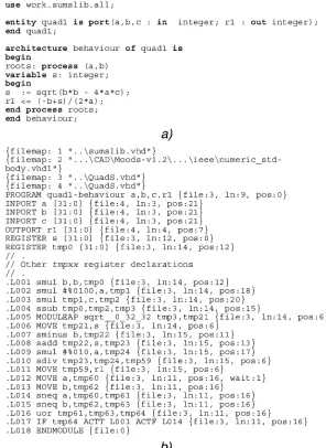
Fig. 1. ICODE generated from VHDL. (a) Generating HDL. (b) Generated intermediate code.
used to create significant designs, such as the SPA [27] using Balsa and a low power pager [28] using Tangram. Another approach is that used by the ACK Framework [29], that parti-tions designs specified using Verilog [30] into separate control and datapath parts. The controller is synthesized using 3-D, while the datapath is synthesized using standard commercial synthesis tools. Theseus Logic, Inc., use a technique known as NCL [31] that also uses commercial synthesis tools, but to create asynchronous circuits that use dual rail encoding and are delay insensitive; however they tend to be some three-to-five times larger than their synchronous equivalent and may have a larger delay and power consumption.
At the behavioral level, Tan has created a tool [32], which allows a limited subset of VHDL to be synthesized onto micropipeline [16] structures, using basic naïve techniques; and [33] which creates optimized controllers for a predefined control data flow graph (CDFG). Finally Bachman [34], [35] has modified many of the standard synchronous synthesis algorithms [8], [9] to be made suitable for the asynchronous domain.
A separate approach to the design of asynchronous circuits is the translation of a synchronous design into an asynchronous one. An approach to this is presented by Cortadella in [36], which allows the registers and clock tree of a synchronous de-sign to be replaced by master slave latches and asynchronous handshaking.
The MOODS synthesis system has been a synthesis research vehicle for over 15 years. Its optimization algorithms work quite differently to many other tools (see above) and including the commercially available Behavioral Compiler from Syn-opsys [37], and Monet from Mentor Graphics [38].
MOODS takes as input the behavior of the system speci-fied in behavioral VHDL [39] or SystemC [40]. (Semantically, there is little to distinguish between the two languages, and throughout the rest of this paper VHDL will be used as the I/O stream, although SystemC could equally well have been used.) Theoutput of the synthesis process is a structural netlist, de-scribing a physical system that displays the desired behavior.
implementa-Fig. 2. Datapath generated from ICODE.
tion. This description is target neutral, in that it applies equally well to a synchronous and asynchronous final implementation.
Section III describes how optimization of the design may be effected by manipulation of the representation of the design. Again, this description is target neutral.
Section IV describes the implementation details of the asyn-chronous synthesis system. (The corresponding minutiae of the synchronous system have been published elsewhere [7], [41].)
[image:3.594.319.532.64.380.2]Finally, in Section V a set of example designs are presented and analyzed, some in detail. The principal point of this section is not to illustrate how good the optimization algorithm is; this has been published extensively [4]–[6], [42], but how the syn-chronous and asynsyn-chronous implementations differ, given the same behavioral input and optimization parameters. The design statistics enumerated in the results are for the same set of de-signs, run under the same optimizer with the same optimization criteria, making them directly comparable.
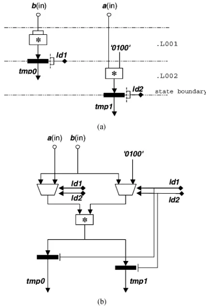
Fig. 3. Sharing functional units. (a) Two multiply operations. (b) Operations shared on one operator.
II. THEGENERICSYNTHESISPROCESS
This section provides a brief description of the overall syn-thesis process, from VHDL behavioral input through (almost) to structural output. The structure produced by this process will be large, slow and inefficient, but functionally correct. The process is generic in that the explanation applies equally and without modification to both synchronous and asynchronous implemen-tations. Specifically, the term “timeslot” doesnotimply the time intervals are of equal length. In a synchronous system, they are. In an asynchronous system, this may not be the case. We also stop short of committing the design to a synchronous or asyn-chronous implementation.
[image:3.594.41.292.65.520.2]SACKERet al.: BEHAVIORAL SYNTHESIS SYSTEM FOR ASYNCHRONOUS CIRCUITS 981
Fig. 4. Controller synthesis.
the quality of the design produced in this manner is generally extremely poor. Any overall aggressive optimization system has no realistic choice but to consider the three activities alongside each other. However, for the sake of clarity, in this section they are described separately.
A. Compilation to Intermediate Code
In common with most synthesis systems, the first step is to take the input description and translate this into a language neu-tral form. We call this ICODE (intermediate code), and it is essentially a hardware assembly language. It has an extremely simple syntax, but whereas most assembly languages use the notion of multiple control threads sparingly if at all, multiple threads are fundamental to the semantics of ICODE.
Fig. 1 shows a small fragment of VHDL describing a system to solve a (cut down) quadratic equation, and the corresponding ICODE.
• For the sake of keeping the example to a manageable size, we have made the process sensitive to only and , and omitted both the evaluation of the second root, and the trap necessary to detect . Note that use of a high level behavioral tool does not (necessarily) absolve the de-signer from the responsibility of defining theentiresystem behavior.
[image:4.594.308.544.67.306.2]• The example uses integer coefficients; by changing the variable declarations and the cell library, the design could equally well generate fixed or floating point or even a com-plex arithmetic implementation. Depending on the level of sophistication (physical size) of the library cells, the de-sign could be made to (automatically) tolerate the condi-tion , by having the low-level cells propagate NaNs.
Fig. 5. Chaining synchronous operations. (a) Two multiply operations: two timeslots. (b) Two multiply operations chained together.
This would generatepredicablebehavior, but is no substi-tute for sensible design.
• Note the back annotation file:3, ln:14, pos:12 associ-ated with each ICODE statement: this allows complete back annotation from the final hardware to the generating HDL source.
• The square root operation is implemented as a function call, the divide as a built in operation, even though the un-derlying functionality is virtually identical. This is a direct reflection of the way the HDL source was written. • Most register declarations(tmpxx)are omitted for the sake
of brevity.tmp61, tmp63, andtmp64are one bit wide; all others are 32 bits.
• The figure shows a single process, and hence the ICODE has a single control thread. (In a multiple process de-sign, the “start” of each process loop would have its own thread.) At this stage, the text can be interpreted as a se-quential set of (labeled) low-level instructions, reading from and writing to “variables.” At the end of each state-ment is an implied “activate next statestate-ment.” Uncondi-tional branching is supported by anACTivatestatement (there are none in Fig. 1.), and conditional branching by
the IF xxx ACTT label ACTF label statement.
(xxx is a Boolean,ACTTmeans “activate if true,”ACTF means “activate if false.”) More complex structures also exist: two multiway branching instructions (SWITCH and DECODE); a detailed description of ICODE is not the focus of this paper.
Fig. 6. Three-dimensional (dynamic) design space trajectory.
B. Scheduling
Scheduling involves mapping the sequence of operations described in the intermediate form onto specific time slots. (For a synchronous implementation, these time slots are naturally clock cycles, but from the dataflow perspective there is no reason why the slots have to be of equal width, which is the ob-servation that opens the door to asynchronous implementation described later). For the simplest possible schedule, we can simply take the instructions of Fig. 1 and map them temporally, as in Fig. 2.
A few points to note.
• The figure represents the data flow within the design. Or-chestrating and controlling the flow of information is im-plied, but not yet specified. In essence, we note that if a variable is written to in one timeslot and read in another, then it must be registered. In Fig. 2, only one thing ever happens in each slot, so each operation has an implied reg-ister associated with it.
• The statement labels of Fig. 1(b) map directly onto the time slots.
• The dataflow associated with the evaluation of the root (.L001 to .L012) is readily identifiable in the figure; the MOVEs of .L012 and .L013, the inequality tests (.L014 and .L015) and the single bit OR (.L016) implement the dataflow aspects of the HDL WAIT construct; in this
case inferred from the process sensitivity list. The “old” values of a and b are stored in tmp60 and tmp62: if either change, the appropriate “not equal” variables (tmp61 or tmp63) will be asserted, triggering the reactivation of the entire instruction sequence by the mechanism described in Section II-E.
C. Allocation
Allocation is the process of mapping the abstract operations of Fig. 2 onto abstract operators. The most naive allocation is to map each abstract operation on to a physical operator. Thus, the system of Fig. 2 would require four multipliers, two subtrac-tors, one adder, and so on. These operators all take up silicon real estate, and clearly such a mapping is ridiculously wasteful. The operators are only in use during the timeslot the operation occupies; for 15 of the 16 timeslots of Fig. 2, each physical oper-ator is doing nothing. Far more sensible is to share the physical operators between timeslots, as in Fig. 3.
SACKERet al.: BEHAVIORAL SYNTHESIS SYSTEM FOR ASYNCHRONOUS CIRCUITS 983
Fig. 7. Chaining asynchronous operations.
of Fig. 3(b) is just over half the size of that in Fig. 3(a). As each timeslot in Fig. 2 has only one operation, this argument can be extended to the point that the entire structure can be realized with exactly one instance of each type of functional unit.
D. Binding
Binding refers to the choice of functional unit used to imple-ment a physical operator; for example, the single multiplier in Fig. 3(b) could be a Booth structure, a carry lookahead, or any of the host of available microarchitectures that will implement the multiply operation. The tradeoffs introduced by this added level of complexity will not be discussed here.
E. Controller Synthesis
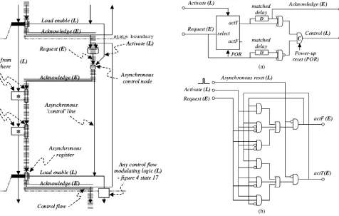
Each operation in Fig. 2 has an implied register after it (explicitly depicted in Fig. 3). Each one of these registers has a ‘load enable’ line, which has to be driven by something. The sequence of load enables that allows the dataflow part of the circuit to deliver the required overall functionality is generated by a state machine: the controller. The controller associated with the dataflow of Fig. 2 is shown in Fig. 4.
The distinction between abstract representation and physical structure is deliberately blurred here, to illuminate how one may be generated from the other: the controller is a graph, where the nodes represent the states of the sequence generator. It is essentially a one-hot machine, which may be thought of as a Petri net.
In reality, in a synchronous system, each controller graph node maps exactly onto a D-type flipflop, which has a clock input, and hence the machine states are of equal length. There
Fig. 8. Asynchronous control cell. (a) Asynchronous control cell. (b) Event-based selector.
is no intrinsic reason why the state intervals should be of equal length: once the logic within a state has completed, the transi-tion to the next state can occur at any time.
The pair of gates in slot 17 are state machine glue logic, also known as one-bit MUX, also known as a switch unit in the Petri net. The salient point is that the behavior of the se-quence generator is altered by a primary input from the dataflow (tmp64 in Fig. 2). On power-up, the generator will cycle through states .L001 to .L016, in accordance with the semantics of the VHDL process. Then the machine will enter a tight “busy loop,” (.L014-.L015-.L016-.L014 ), continually checking to see ifa orbhas changed. (The VHDL “wait” construct.) As and when either of these changes, the sequence diverts up to state .L001 again, and the process body is reevaluated.
III. OPTIMIZATION
It is worth reemphasizing here that the term “timeslot” does not necessarily imply time intervals of equal length in this ex-planation.
Behavioral synthesis is an application that has been ret-rofitted onto hardware description languages, and one of the consequences of this is that any sensible optimizing synthesis system almost inevitably either breaks the temporal semantics of the input language or places severe restrictions on its use. This is the price that has to be paid for allowing the optimizer the freedom to do its work.
[image:6.594.59.535.65.368.2] [image:6.594.43.299.65.360.2]Fig. 9. Asynchronous functional unit.
Fig. 10. The asynchronous register. (a) Asynchronous register. (b) Double edge flipflop.
although sometimes delay is data-dependant). Other attributes, such as power distribution and RF spectra can only be evaluated by dynamic analysis, i.e., simulation: they depend critically on the actual excitation of the system. Irrespective of this, the term “optimization” in the context of behavioral synthesis means moving the metrics toward some user-defined target, while at the same time maintaining the overall functional behavior of the system. One such “peephole” optimization was shown in Fig. 3: the multiplier was shared, thereby saving a considerable amount of area. Other transformations to the structure have different effects. Consider Fig. 5(a), which is another fragment of the overall system of Fig. 2. This is trivially transformed into the structure of Fig. 5(b). The functional behavior is the same, but the area and delay metrics are considerably different:
1) Temporal: The two operations have been pushed into the same timeslot, so ostensibly for synchronous design, the speed
Fig. 11. Operations in parallel: neither operator shared.
has doubled, unless the propagation delay of the chained opera-tions is larger than the slot period. In which case, the clock may have to be slowed, which may or may not reduce the overall process loop delay. Another way round the problem (if the in-structions concerned are not on the critical path) is to cycle-skip that particular pair of operations.
2) Spatial: We have removed a register, and reduced the number of states in the controller, both of which will reduce the overall area. If the controller is one-hot, each state will have a linear area cost. If it is an encoded architecture, the spatial saving is likely to be logarithmic with the total state count. Note also that the variabletmp1 is now a piece of wire, not a register. The most important consequence of applying this transforma-tion, however, is that by so doing we have prevented the possi-bility of sharing the operations on one operator. We cannot now use the transform outlined in Fig. 3, because both multiplica-tions take place in the same timeslot, so we have no choice but to use two discrete multipliers.
[image:7.594.57.268.209.525.2]SACKERet al.: BEHAVIORAL SYNTHESIS SYSTEM FOR ASYNCHRONOUS CIRCUITS 985
Fig. 12. Sharing units. Multiplexing in time, the asynchronous version of Fig. 3(b).
Two optimization techniques have been outlined in this section and many others exist [41]; the topic of behavioral optimization is immense, and it is not the purpose of this paper to contribute to that field. The point illustrated by this section is that optimizing almost inevitably involves resolving, by some mechanism, conflicting pressures between extremely diverse metrics.
Finally, it is worth reinforcing that all practical behavioral synthesis breaks the semantics of the generating HDL source. The concept of a process is common to all hardware description languages: it enables the designer to separate out the temporal and functional aspects of a description. A process is a loop, con-taining a sequence of calculations of arbitrary complexity, that “executes” in zero time. Real time passes, only at “wait” or the equivalent statements. Synthesis is the process of automatically translating a behavioral description into a structure. It follows, then, that the behavior of the actual synthesized structure only approaches that described by the HDL as the timeslot period approaches zero, which it clearly cannot do in reality.
IV. ASYNCHRONOUSSYNTHESIS
[image:8.594.42.284.66.392.2]Any synthesized system, is simply an automatically generated network, where the flow of data through the network is regulated such that the behavior of the system is what the user/designer wanted. In a synchronous system, the dataflow is regulated by a discrete controller, itself controlled by a fixed clock. Each
Fig. 13. The asynchronous control DEMUX.
Fig. 14. Asynchronous dataMUX.
[image:8.594.323.526.373.628.2]controller with a “stage complete” flag, we effectively have an asynchronous implementation.
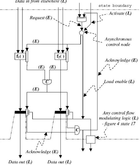
The “flow of control” passes through the control cellsandthe datapath units: see the thick grey arrow in Fig. 7. The details will be explained later.
In principle, this is all that is required to produce a function-ally correct structure, but in practice there are a number of other modifications worthy of note.
A. Optimization—Measure of Goodness
The optimization function attempts to minimize some “mea-sure of goodness” (MOG) numerically defining the quality of the design. (In this paper, we are largely restricting this to the area and delay of the design.) The derivation of the MOG changes if we move to an asynchronous implementation:
1) Area: The functional units are now bigger, not only do they have to support the defined functionality, but they also are now responsible for generating the “stage complete” signal, and reacting to the “request” input.
The control cells have a completely different internal structure to their synchronous counterparts (see Section IV-B), and hence will have a different area. In the general case, it is impossible to predict whether the synchronous or asynchronous controller will be smaller. For a synchronous system, the architecture of the controller is usually one-hot for less than about eight states (the size of the controller grows roughly linearly with the number of states), or encoded (where the size grows logarithmically with state count) for larger systems. In an asynchronous system, the same tradeoff exists, but the size of the larger encoded system depends significantly on the number of dummy cycles1
necessary to avoid race hazards, which makes the size difficult to predict from abstract reasoning. It is partly for this reason that we have chosen to use the distributed one-hot asynchronous architecture for the controller.
2) Delay: For a synchronous system, the delay of a process is the critical path length (including any knownloop informa-tion) multiplied by the clock period.
For an asynchronous system, it is simply the sums of the state delays (including as before any known loop information) in the critical path.
1In asynchronousstate machine, the actual bit patterns used to distinguish
the states (the state vector) are irrelevant from the point of view of the behavior of the machine. The state–state transitions are dictated by the “glue logic” and orchestrated by the clock. In anasynchronousmachine, adjacent state codes must have a Hamming distance of exactly 1, to avoid race hazards in the combinational logic. If this is not possible, a dummy cycle (state) must be inserted to ensure that everystate transition satisfies the above criteria. Consider the trivial example of a three-state machine, cycling in a loop. With a synchronous implementation, without loss of generality, the state encoding could be A(00) ) B(01) ) C(10) ) A(00) and so on. This coding
cannotbe used in an asynchronous machine, because theB ) Ctransition cannot be realized in combinational logic without a race. To realize this particular example in asynchronous logic, a dummy cycle would be inserted to eliminate the race: A(00) ) B(01) ) C(11) ) dummy(10) ) A(00). The dummy state is unconditionally unstable, and once entered, transitions
[image:9.594.305.557.64.301.2]immediately to its successor state. Note that in this example, the only cost of this is a slight increase in gate count and a slightly longer delay in the C ) A transition. However, in a more complex system, it may be necessary to insert multiple chainsof dummy cycles, and it may also be necessary to increase the lengthof the state vector well abovelog (total states) to accommodate this. These latter points make it virtually impossible to estimate the size of the machine without actually designing it in totality.
Fig. 15. AsynchronousIFrealization (compare with Fig. 4).
Fig. 16. Extension of the IF construct (Fig. 15) to the generic select (SWITCH-CASE) construct.
B. Controller
The synchronous control cells (see Fig. 4) are simply D-type flip-flops, with a reducing-ORfunction on the inputs (Fig. 4, state 14, for example). The flow of control is trivially modulated using a switch configuration like that shown in Fig. 4, state 17. The clock and global reset is implied. Essentially, two signals go from control state to control state: theclockand thecontrol line.
With an asynchronous implementation, the controller state machine is similar in topology, a sequence of one-hot cells, but there is no clock, and the cells communicate with each other and the datapath using request–activate handshakes. Fig. 7 shows an example of a single state containing a chain of two multiplies [compare this with Fig. 5(b)]. Again, two signals go from con-trol state to concon-trol state:acknowledgeandcontrol.
[image:9.594.312.542.349.486.2](level-SACKERet al.: BEHAVIORAL SYNTHESIS SYSTEM FOR ASYNCHRONOUS CIRCUITS 987
TABLE I
SYNCHRONOUSPORTFOLIODESIGNSTATISTICS
based)XORgate symbol in Fig. 7 implements the reducing-OR function for events. The internal structure of the control node is shown in Fig. 8: compare the structure of the event based switch [Fig. 8(b) [43]] with the level based synchronous version (Fig. 4 state 17). The Muller-C gate in Fig. 8(a) implements the event-based reducing-ANDfunction [16], [43].
C. Datapath Units
The asynchronous datapath units are simply synchronous combinational units with a disjoint event based network in parallel providing the “all done” handshake information, see Fig. 9. This gives the same worst case performance for a single
DPU as for synchronous. However, if a cell library exists that contains units with completion detection, these could be used instead to give average case performance for each DPU. Note that if a datapath unit has been shared, then a demultiplexer is required for the output acknowledge in order to prevent acknowledge events being issued to parts of the circuit where they are not required.
D. Registers
TABLE II
ASYNCHRONOUSPORTFOLIODESIGNSTATISTICS
Fig. 10 (taken from .[44]). The event selector box in Fig. 10(a) is the same device as used in the controller, shown in Fig. 8(b).
E. Signal Encoding
There exist several popular design methodologies for the de-sign of asynchronous systems: these affect how handshaking is performed and how data is represented. For the handshaking protocol, the main choice is between two-and four-phase or re-turn-to-zero handshaking protocols [45], [46]. For four phase, there are three variations on the theme: early, broad and late data. These differ in the phase in which the data is valid.
SACKERet al.: BEHAVIORAL SYNTHESIS SYSTEM FOR ASYNCHRONOUS CIRCUITS 989
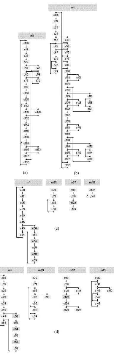
Fig. 17. The quadratic equation solver control graphs. (a) Synchronous target, optimized for area. All procedure calls inlined. (b) Asynchronous target, optimized for area. All procedure calls inlined. (c) Synchronous target, optimized for area. Procedure calls not inlined. (d) Asynchronous target, optimized for area. Procedure calls not inlined.
tighter timing constraints when used with bundled handshake signals, as this configuration is not delay insensitive.
We use single rail encoding with two phase signaling, which in principle puts the correct functioning of the circuit at the mercy of unbalanced delays introduced by” (APR) sub-system; however, conservative choice of the delay parameters [Figs. 8(a), 9, and 10(b)] mean that this has not been a problem to date.
F. Optimization Structures
Practical optimization relies for the main in taking a naive dataflow and schedule (Fig. 2, for example) and perturbing it.
Two principal techniques are used: first, moving the opera-tions between timeslots. (Where the operaopera-tions have some data dependency, this is known aschaining, Fig. 7. Where there is no dependency, the process is called grouping. Obviously, groups may contain chains.) This effectively changes theschedule, and affects the overall latency of the design.
Second, individual abstract operations may be mapped onto the same physical operator (Fig. 3)—this changes the alloca-tion and affects primarily the overall area of the design. The tradeoffs between these two operations alone are nontrivial and nonmonotonic. Introducing further optimization criteria (for ex-ample, Fig. 6 [6]) makes the situation even more complex.
Chaining, grouping, and sharing are all valid optimization techniques in both the synchronous and asynchronous domains. Figs. 7–10 show asynchronous chaining, and the associated structures, which are relatively straightforward.
Fig. 11 shows two functions: and , grouped in a single state. Although there are no data dependencies between and , note that it is still necessary to synchronize the re-sults together at the state boundary. The reason for this is as fol-lows: although there is guaranteed to be no data feedbackwithin a state (the I/O dataflow relationships of a state can always be written as purely combinational Boolean expressions) it is en-tirely possible that feedbackarounda state (that is, its output connected to its inputs) can occur. If there is more than one output to a state, this data can become temporally misaligned, with unpredictable dataflow results.
Datapath unit sharing, the asynchronous counterpart of Fig. 3(b), is shown in Fig. 12. Note, it is no longer possible or sensible to extend the state boundaries to the dataflow part of the circuit.
The circuit is intrinsically safe, in that there is no possibility of the two control state competing for the single resource. This safety derives not from the local circuit topology, but from the overall organization of the synthesis system: if the threat of com-petition exists (which can be determined from a static analysis of the dataflow) then the abstract operations are not shared on the resource, so there is no problem.
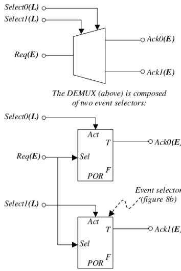
Unit sharing requires two more specialized subunits: the asynchronous control DEMUX (Fig. 13) and the asynchronous dataMUX(Fig. 14).
Note there is no such thing as an asynchronous data DEMUX (it is a piece of wire) and the asynchronous controlMUXis a nonsensical concept.
Fig. 18. Design space for the quartic equation solver, various static optimization criteria. (a) Synchronous target, procedure calls not inlined. (b) Asynchronous target, procedure calls not inlined. Note: “Delay” and “Both” coincide. (c) Synchronous target, procedure calls not inlined. Note: “‘Delay” and “Both” coincide. (d) Asynchronous target, procedure calls inlined.
This is trivially extended (Fig. 16) to support the concept of a generic select (SWITCH-CASE) construct.
V. RESULTS
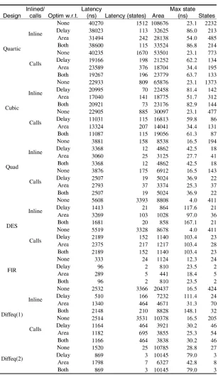
Statistics relating to the synthesis of six behavioral designs are shown in Tables I and II. All the designs are defined in VHDL, and consist of (without loss of generality) a single process with a hierarchy of procedure and function calls under it. The designs are: 1) a quadratic equation solver [47] (which includes a square root and divide); 2) a cubic equation solver [47] (which includes square and cube roots, and forward cosines); 3) a quartic equation solver [47] (which also contains square and cube roots, and forward cosines); 4) the DES block encryption algorithm.[48]; 5) two versions of a differential equation solver as discussed in Section V-A; and 6) a finite impulse response discrete filter. Each of these designs were synthesized forallcombinations of the following parameters:
• synchronous–asynchronous;
• optimized with respect to nothing/area/delay/both area and delay;
• procedure and function inlining or not.
(The filter has no hierarchy, so the inlined–not inlined results are identical.) Table I shows the synchronous results, Table II the asynchronous.
Inlined–calls indicates if the design hierarchy is flattened be-fore optimization. (Flattening enablesconsiderably more unit sharing, both spatially and temporally, but usually from a larger initial spatial configuration.)
Optim w.r.t. indicates the static optimization criteria asserted by the user.
Latency (ns) is the length of the critical path through the design, in nanoseconds, when the clock is run at its maximum possible value (column Max clk).
Latency (states) is the number of states in the critical path. Area is a relative figure; the cell library used was designed for Xilinx Virtex devices [49], the figures refer to the estimated slice count.
Max clk (ns) is the period of the fastest clock that can be used to drive the system. Another way of looking at it is as the longest combinational logic delay through any state (minus the register setup time).
SACKERet al.: BEHAVIORAL SYNTHESIS SYSTEM FOR ASYNCHRONOUS CIRCUITS 991
Fig. 19. Design space for the DES encryption block, various static optimization criteria.
Waste in a synchronous design, all states have the same (tem-poral) width, but the delay of the functional units with that state will usually be less than that width. (Except for the slowest, nat-urally, as thisdictates the maximum clock speed.) Thus most states will have a nonzero “dead time.” The waste column is the sum over all the states of the dead time. (It isnotthe sum over the critical path.) The average waste figure of the 44 entries is 0.65, i.e., 65% of the elapsed time is spent doing nothing.
It is tempting, at first sight, to attempt a comparison between the wasted space in a synchronous design and the performance increase in the asynchronous counterpart. However, they are not directly comparable, for two reasons: First, the optimizer will have made different atomic decisions as the relative timings change in the two regimes, i.e., the scheduling and allocation
will be different (see Fig. 11). Second, thewaste metric (see Table I) refers to the total waste summed over all states of the design; the latency figures refer to the states in the critical path. Max state (ns) is the length of the longest state in an asyn-chronous design. (This may or may not be on the critical path.)
A. Optimization: Scheduling
Fig. 20. Wasted time in the synchronous inlined cubic equation solver.
and asynchronous platforms has resulted in significantly dif-ferent structures for the implementations. Closer examination of the designs indicate that this effect arises from two causes:
• For an asynchronous target, there is less pressure to chain functional units, because the incremental effect on the la-tency is negligible.
• For a synchronous target, preemptive calculation costs area, but no time. For the asynchronous counterpart, it costs time. Thus, it is better to have lots of short asynchronous states. The design generating the DIFFEQ(2) results in Tables I and II is taken from [50]. It solves a fixed equation
with a fixed method (forward Euler) and so is intrinsically much smaller and simpler than DIFFEQ(1), which supports solution via Euler, modified Euler and Runge-Kutta [51]. It is interesting to note that latency when optimized for area is greater than the naive (unoptimized) implementation because theMUXlatency is greater than the control overhead of having every operation in its own state.
B. Optimization: Static Design Space
Fig. 18 shows the static design spaces for the quartic equa-tion solver, again for the four combinaequa-tions of (inlined–unin-lined)/(synchronous–asynchronous) solution.
On each design space four points are shown: a) for a naïve de-sign with no optimization; b) for a dede-sign optimized to minimize delay; c) for a design optimized to minimize area; and d) for a design optimized to minimize both delay and area. The naive design is usually the largest and slowest point (top right hand corner of the design space). Note that the naïve asynchronous circuits have a significantly smaller latency to that of their syn-chronous equivalent, despite the schedule being the same as if no optimization has occurred, due the large waste of an unuti-lized synchronous system. Similarly, the design optimized for minimum area is the point nearest the horizontal axis; however the design optimized for minimum latency is not always. This is
due to inaccuracies in estimating the latency during synthesis, as the number of iterations around loops that are not bounded (i.e., they are data dependant) is usually impossible to infer. The final optimization is a compromise between optimizing for minimum delay and minimum area.
The uninlined designs have smaller area than their inlined equivalents. An inlined design reproduces the data and con-trol path for each procedure, which has the potential to achieve more optimization across procedural boundaries, however in this case the inherently shared uninlined procedure modules are smaller. The asynchronous designs are faster than their syn-chronous equivalents except for the case of the uninlined de-sign optimized to minimize both area and delay. On average the quartic asynchronous designs require 66% of the time of their synchronous equivalents.
Fig. 19 shows the design space for the DES block. The dra-matic difference between synchronous and asynchronous la-tency derive from the internal structure of the algorithm: DES comprises mainly table lookups (which are effectively bit shuf-fles) and theXORoperation. The numerous bit-shuffling opera-tions further resolve to a series of bit-wise concatenaopera-tions. In a synchronous implementation, this is realized, literally, as pieces of wire; the cost in terms of both area and delay is completely negligible. In an asynchronous implementation, each concate-nation requires asynchronous control, which as a penalty asso-ciated with it. Finally, theXORoperation itself is intrinsically slower asynchronously than it is synchronously.
C. Temporal Utilization (Waste)
SACKERet al.: BEHAVIORAL SYNTHESIS SYSTEM FOR ASYNCHRONOUS CIRCUITS 993
of the way from the left axis) dictates the fastest clock that can be used for the entire design. The optimizer attempts to chain operations (combining control states) to decrease the amount of low occupancy states in the design, but obviously it can only do so where data or control flow conflicts permit. Of the 114 states in the design, a few have extremely low occupancy; these are used to move data before–after entering–leaving a control loop. No temporal optimization is possible here.
VI. FINALREMARKS
A technique for the behavioral synthesis of asynchronous cir-cuits has been presented, and the physical parameters of the re-sulting implementations compared to a synchronous equivalent. The technique is based on methods established for use in syn-thesizing synchronous circuits, which are modified to support the design of asynchronous circuits.
The results show that the asynchronous circuit generated can perform significantly faster than the synchronous equivalent, at the cost of extra area, which is to be expected. However, thus is by no means guaranteed, and the only real conclusion that can be drawn is that the availability of a choice between syn-chronous and asynsyn-chronousmayallow an implementation with significantly different static parameters. The ability of advanced behavioral synthesis tools to explore design space from a target neutral specification means that designers can easily have the best of both worlds: architectural exploration means just that the designer can trivially ask the tools what the best solution is, and simply go with it.
Future work is focused on the idea of extending the concept further by allowing large “islands of synchronicity” to exist in an asynchronous “sea,”where the boundaries between the do-mains are identified and handledautomaticallyby the synthesis system, transparently to the user.
REFERENCES
[1] E. Brunvand, S. Nowick, and K. Yun, “Practical advances in asyn-chronous design and in asynchronous/synchronous interfaces,” presented at theProc. Design Automation Conf., Piscataway, NJ, 1999. [2] S. Hauck, “Asynchronous design methodologies: An overview,”Proc.
IEEE, vol. 83, pp. 69–93, 1995.
[3] C. J. Myers,Asynchronous Circuit Design. New York: Wiley, 2001. [4] A. D. Brown, K. R. Baker, and A. C. Williams, “Online testing of
stat-ically and dynamstat-ically scheduled synthesized systems,”IEEE Trans. Computer-Aided Design, vol. 16, pp. 47–57, Jan., 1997.
[5] Z. A. Baidas, A. D. Brown, and A. C. Williams, “Floating point be-havioral synthesis,”IEEE Trans. Computer-Aided Design, vol. 20, pp. 828–839, July.
[6] A. C. Williams, A. D. Brown, and M. Zwolinski, “Simultaneous opti-mization of dynamic power, area and delay in behavioral synthesis,” in
Proc. Inst. Elect. Eng. Computers Digital Techniques, vol. 147, 2000, pp. 383–390.
[7] K. R. Baker and A. J. Currie, “Multiple objective optimization in a be-havioral synthesis system,” inProc. Inst. Elect. Eng., vol. 140, 1993, pp. 253–260.
[8] M. C. McFarland, A. C. Parker, and R. Camposano, “Tutorial on high-level synthesis,” presented at theDesign Automation Conf., 1988. [9] G. De Micheli,Synthesis and Optimization of Digital Circuits. New
York: McGraw-Hill, 1994.
[10] H. Shiraishi and F. Hirose, “Efficient placement and routing techniques for master slice LSI,” presented at theDesign Automation Conf., Min-neapolis, MN, 1980.
[11] P. G. Paulin and J. P. Knight, “Force-directed scheduling for the behav-ioral synthesis of ASIC’s,”IEEE Trans. Computer-Aided Design, vol. 8, pp. 661–679, June, 1989.
[12] T. Yoshimura and E. S. Kuh, “Efficient algorithms for channel routing,”
IEEE Trans. Computer-Aided Design, vol. 1, pp. 25–35, Jan., 1982. [13] S. B. Furber, J. D. Garside, S. Temple, J. Liu, P. Day, and N. C. Paver,
“AMULET2e: An asynchronous embedded controller,” presented at the
Advanced Research in Asynchronous Circuits and Systems, Eindhoven, The Netherlands, 1997.
[14] S. B. Furber, P. Day, J. D. Garside, N. C. Paver, and J. V. Woods, “AMULET1: A micropipelined ARM,” presented at theIEEE Com-puter Conf. (COMPCON), San Francisco, CA, 1994.
[15] J. D. Garside, W. J. Bainbridge, A. Bardsley, D. M. Clark, D. A. Ed-wards, S. B. Furber, J. Liu, D. W. Lloyd, S. Mohammadi, J. S. Pepper, O. Petlin, S. Temple, and J. V. Woods, “AMULET3i—An asynchronous system-on-chip,” presented at theAsynchronous Circuits and Systems, 2000.
[16] I. E. Sutherland, “Micropipelines,” Commun. ACM, vol. 32, pp. 720–738, 1989.
[17] T. Murata, “Petri nets: Properties, analysis and applications,” Proc. IEEE, vol. 77, pp. 541–580, 1989.
[18] J. Cortadella, M. Kishinevsky, A. Kondratyev, L. Lavagno, and A. Yakovlev, “Petrify: A Tool for Manipulating Concurrent Specifications and Synthesis of Asynchronous Controllers,” Departament d’Arquitec-tura de Computadors, Universitat Politecnica de Catalunya, Tech. Rep., 1996.
[19] R. M. Fuhrer, N. K. Jha, S. N. Nowick, B. Lin, M. Theobald, and L. Plana,MINIMALIST: An Environment for the Synthesis, Verification, and Testability of Burst-Mode Asynchronous Machines, 1999. [20] K. Y. Yun and D. L. Dill, “Automatic synthesis of extended burst-mode
circuits: Part I (specification and hazard-free implementations),”IEEE Trans. Computer-Aided Design, vol. 18, pp. 101–117, Jan., 1999. [21] , “Automatic synthesis of extended burst-mode circuits: Part II
(au-tomatic synthesis),”IEEE Trans. Computer-Aided Design, vol. 18, pp. 118–132, Jan., 1999.
[22] A. Bardsley and D. A. Edwards, “The balsa asynchronous circuit syn-thesis system,” inProc. Forum Design Languages, Tübingen, Germany, 2000.
[23] A. Bardsley, “Implementing Balsa Handshake Circuits,” Ph.D. disserta-tion, Univ. Manchester, Manchester, U.K., 2000.
[24] J. Kessels and A. Peeters, “The tangram framework (embedded tutorial): Asynchronous circuits for low power,” inProc. Asia South Pacific De-sign Automation Conf., Yokohama, Japan, 2001.
[25] C. A. R. Hoare, “Communicating sequential processes,”Commun., vol. 21, pp. 666–677, 1978.
[26] Occam 2 Reference Manual. Englewood Cliffs, NJ: Prentice-Hall, 1988.
[27] L. Plana, P. A. Riocreux, W. J. Bainbridge, A. Bardsley, J. D. Garside, and S. Temple, “SPA—A synthesisable amulet core for smartcard ap-plications,” inProc. Int. Symp. Asynchronous Circuits Systems, Man-chester, U.K., 2002.
[28] J. Kessels and P. Marston, “Designing asynchronous standby circuits for a low-power pager,” inProc. IEEE, Feb. 1999, pp. 257–267.
[29] H. Jacobson, E. Brunvand, G. Gopalakrishnan, and P. Kudva, “High-level asynchronous system design using the ACK framework,” inProc. Int. Symp. Advanced Research Asynchronous Circuits Systems, Eilat, Is-rael, 2000.
[30] IEEE Standard Hardware Description Language Based on the Verilog Hardware Description Language, 1995. IEEE Std. 1364-1995. [31] M. Ligthart, K. Fant, R. Smith, A. Taubin, and A. Kondratyev,
“Asyn-chronous design using commercial HDL synthesis tools,” inProc. Int. Symp. Advanced Research Asynchronous Circuits Systems, Eilat, Israel, 2000.
[32] S.-Y. Tan, S. B. Furber, and W.-F. Yen, “The Design of an asynchronous VHDL synthesizer,” inProc. Design, Automation Test Europe, Los Alamitos, CA, 1998.
[33] M. Theobald and S. M. Nowick, “Transformations for the synthesis and optimization of asynchronous distributed control,” inProc. Design Au-tomation Conf., Las Vegas, NV, 2001.
[34] B. M. Bachman, “Architectural-Level Synthesis of Asynchronous Sys-tems,” Masters Thesis, Univ. Utah, Salt Lake City, UT, 1998. [35] B. M. Bachman, Z. Hao, and M. C. J, “Architectural synthesis of timed
asynchronous systems,” inProc. IEEE Int. Conf. Computer Design (ICCD), Austin, TX, 1999.
[37] Behavioral Compiler User Guide Synopsys, 2000. Reference Manual Version 2000.11.
[38] Monet, www.mentor.com/monet, 1998. Mentor Graphics.
[39] IEEE Standard VHDL Reference Manual, IEEE Std 1076-1993, 1993. [40] Functional Specification for SystemC 2.0, 2001.
[41] A. C. Williams, “A Behavioral VHDL Synthesis System Using Data Path Optimization,” Ph.D. dissertation, Univ. Southampton, Southampton, U.K., 1997.
[42] A. D. Brown, A. C. Williams, and Z. A. Baidas, “Hierarchical module expansion in a VHDL behavioral synthesis system,” inElectronic Chips & Systems Design Languages, J. Mermet, Ed. Norwell, MA: Kluwer, 2001, pp. 249–260.
[43] K. Maheswaran and V. Akella, “Hazard-Free Implementation of the Self-Timed Cell Set in a Xilinx FPGA,” Univ. Calif. Davis, Davis, CA, Tech. Report, 1994.
[44] M. Pedram, Q. Wu, and X. Wu, “A new design for double edge triggered flip-flops,” inProc. Asia South Pacific Design Automation Conf., Yoka-hama, Japan, 1998, pp. 417–421.
[45] S. S. Appleton, A. V. Morton, and M. J. Liebelt, “Two-phase asynchronous pipeline control,” inProc. Int. Symp. Advanced Research Asynchronous Circuits Systems, Eindhoven, The Netherlands, 1997. [46] S. B. Furber and P. Day, “Four-phase micropipeline latch control
cir-cuits,”IEEE Trans. VLSI Syst., vol. 4, pp. 247–253, Aug., 1996. [47] Schaum’s Outline Series Mathmatical Handbook of Formulas and
Tables, McGraw-Hill, New York, 1968.
[48] “Designing DES with MOODS,” LME Design Automation Ltd., In-ternal Report, 2001.
[49] “The Programmable Logic Data Book,” Xilinx Incorporation, 2000. [50] K. Y. Yun, P. A. Beerel, V. Vakilotojar, A. E. Dooply, and J. Areceo,
“The design and verification of high-performance low-control-overhead asynchronous differential equation solver,” inIEEE Trans. VLSI Syst., vol. 6, Dec. 1998, pp. 1–14.
[51] J. Press, S. A. Teukolsky, W. T. Vetterling, and B. P. Flannery,Numerical Recipes in C—The Art of Scientific Computing, 2nd ed. Cambridge, U.K.: Cambridge Univ., 1992.
Matt Sackerreceived the B.Eng. in electronic engineering from the Univer-sity of Southampton, Southampton, U.K., in 2000, and is currently working toward the Ph.D. degree with the Electronic System Design Group at the same university.
He worked in the DSP group of CRL Ltd, and now works as a Consultant for Detica Ltd., Guildford, U.K.
Andrew D. Brown(M’90–SM’96) was born in the U.K. in 1955. He received the B.Sc. degree (Hons.) in physical electronics and the Ph.D. degree in mi-croelectronics from Southampton University, Southampton, U.K., in 1976 and 1981, respectively.
He was appointed Lecturer in electronics at Southampton University in 1981, a Senior Lecturer in 1989, a Reader in 1992, and appointed to an established chair in 1998. He was a Visiting Scientist at IBM, Hursley Park, U.K., in 1983, a Visiting Professor at Siemens NeuPerlach, Munich, Germany, in 1989, and a Visiting Professor at Trondheim University, Trondheim, Norway, in 2004. He is currently Head of the Electronic System Design Group, Electronics Depart-ment, Southampton University. The research interests include all aspects of sim-ulation, modeling, synthesis, and testing.
Dr. Brown is a Fellow of the IEE, a Chartered Engineer, and a European Engineer.
Andrew J. Rushtonreceived the B.Sc. and Ph.D. degrees in electronics from the Department of Electronics and Computer Science at Southampton Univer-sity, Southampton, U.K., in 1983 and 1987, respectively.
Between 1988 and 1992, he was with Plessey Research Roke Manor (now part of Siemens), involved in RTL Synthesis. He was a founding member of TransEDA Limited, joining the company in 1992 and working for them as Re-search Manager until 1999. During this time, he worked on RTL synthesis, HDL verification and VHDL compilers. From 1999 to 2001, he was with LME De-sign Automation, working on the commercialization of a behavioral synthesis system. Currently, he is a Research Fellow in the School of Electronics and Computer Science, Southampton University. His interests include VHDL, com-piler design, behavioral synthesis, RTL synthesis and C++ library development. He is the author ofVHDL for Logic Synthesis(New York: Wiley, 1998).
Peter R. Wilsonreceived the B.Eng. degree in electrical and electronic en-gineering and the Postgraduate Diploma in digital systems enen-gineering from Heriot-Watt University, Edinburgh, Scotland, in 1988 and 1992, respectively, an M.B.A. degree from the Edinburgh Business School, Edinburgh, in 1999 and the Ph.D. degree from the University of Southampton, Southampton, U.K., in 2002.
He is currently a Senior lecturer with the School of Electronics and Com-puter Science, University of Southampton. From 1988 to 1990, he worked with the Navigation Systems Division of Ferranti plc., Edinburgh, Scotland, on fire control computer systems. In 1990, he joined the Radar Systems Division of GEC-Marconi Avionics, Edinburgh, Scotland. From 1990 to 1994 he worked on modeling and simulation of power supplies, signal processing systems, Servo and mixed technology systems. From 1994 to 1999, he worked as a European Product Specialist with Analogy Inc., Swindon, U.K. During this time he devel-oped a number of models, libraries, and modeling tools for the Saber simulator, especially in the areas of power systems, magnetic components and telecommu-nications. Since 1999, he has been with the Electronic Systems Design group, University of Southampton. His current research interests include modeling of magnetic components in electric circuits, power electronics, renewable energy systems, VHDL-AMS modeling and simulation, and the development of elec-tronic design tools.