On the computation of the multivariate structured total least
squares estimator
Ivan Markovsky
1;∗;†, Sabine Van Huel
1and Alexander Kukush
21K.U. Leuven;ESAT-SCD;Kasteelpark Arenberg 10;B-3001 Leuven-Heverlee;Belgium 2National Taras Shevchenko University;Vladimirskaya st. 64;01601;Kiev;Ukraine
SUMMARY
A multivariate structured total least squares problem is considered, in which the extended data matrix is partitioned into blocks and each of the blocks is Toeplitz=Hankel structured, unstructured, or noise free. Two types of numerical solution methods for this problem are proposed: (i) standard local optimization methods in combination with ecient evaluation of the cost function and its rst derivative, and (ii) an iterative procedure proposed originally for the element-wise weighted total least squares problem. The computational eciency of the proposed methods is compared with this of alternative methods. Copyright? 2004 John Wiley & Sons, Ltd.
KEY WORDS: parameter estimation; total least squares; structured total least squares; system identi-cation
1. INTRODUCTION
1.1. Identication of a moving average time series model as an STLS problem
We introduce the structured total least squares (STLS) problem by an example. Consider the moving average time series model
a(i)x(1) + a(i−1)x(2) = b(i) for i= 1; : : : ; m (1)
∗Correspondence to: I. Markovsky, K.U.Leuven, ESAT-SCD, Kasteelpark Arenberg 10, B-3001 Leuven-Heverlee, Belgium.
†E-mail: [email protected]
Contract=grant sponsor: Research Council KUL; contract=grant numbers: GOA-Mesto 666, IDO=99=003, IDO=02=009
Contract=grant sponsor: Flemish Government FWO; contract=grant numbers: G.0200.00, G.0078.01, G.0407.02, G.0269.02, G.0270.02
Contract=grant sponsor: AWI Contract=grant sponsor: IWT
Contract=grant sponsor: Belgian Federal Government; contract=grant number: IUAP IV-02; IUAP V-22 Contract=grant sponsor: EU
The vector x:= [x(1) x(2)] of the weights is the parameter vector of the model, {a(i)}m i=1
is the input time series, {b(i)}m
i=1 is the output time series, and a(0) is the initial condition.
With A:=
a(1) a(0)
a(2) a(1) ..
. ...
a(m) a(m−1)
and b:= b(1) b(2) .. . b(m)
the time-series model (1) is written as a linear system of equations Ax= b, with structured data matrix C:= [ A b] ( A Toeplitz and b unstructured). The structure parameter vector is the vector
p:= [ a(0) a(1) · · · a(m) b(1) · · · b(m) ]
i.e. there exists a mapping S:R2m+1→Rm×3 (linear, in the example), such that C=S( p).
Suppose that we measure the input, the output, and the initial condition with additive noise: p= p+ ˜p. Here p is the true value and ˜pis the measurement noise that is assumed to be a realization of a zero mean random vector with known covariance matrix2I. The noise level
2 is not given but is estimated on the way of solving the problem.
We consider the following system identication problem: given the measurementsp, nd an estimate of the true value of the model parameter vector x (i.e. Ax= b). With [A b] :=S(p), in general, we have an incompatible system of equations Ax≈b. Thus, the considered iden-tication problem is equivalent to the problem of solving the over-determined system of equations Ax≈b with structured data matrix C:= [A b].
One can take as an estimate the solution of the least squares (LS) problem
min x;bb
2
2 s:t: Ax=b−b
It is well known, however, that this approach leads to a biased estimate, see Reference [1]. In Reference [2], a bias corrected least squares estimator is proposed that leads to a consistent estimator. Another approach that yields a consistent estimator, see Reference [3], is the total least squares (TLS) method [4, 5],
min
x;A;b[ A b]
2
F s:t: (A−A)x=b−b (2)
Both the bias corrected LS and the TLS methods, however, ignore the structure in the data matrixC, i.e. the corrected data matrices [A b−b], in the LS case, and [A−A b−b], in the TLS case, do not necessarily have the required structure. Taking into account the structure leads to statistically more ecient estimates and also to computationally faster algorithms.
A TLS-like problem, that performs minimization (2) over the class of matrices with the required structure is
min x;pp
2
2 s:t: S(p−p)
x
−1
= 0
is proven in References [6, 7]. The fact that the STLS estimator is consistent and ecient under mild assumptions, satised in many applications, and the possibility to design ecient algorithms by exploiting the structure on the level of the computations makes the STLS problem attractive.
1.2. The multivariate STLS problem
Other applications, e.g. nite impulse response (FIR) model identication, autoregressive mov-ing average (ARMA) model identication, and approximation of a Hankel matrix by a lower rank Hankel matrix (Hankel low rank approximation), can be formulated and solved as STLS problems. For more examples, see References [8, 9]. Dierent applications, however, result in dierent structures of the extended data matrix C. Also some applications, e.g. the Hankel low rank approximation problem, require a multivariate linear model AX≈B. We dene a multivariate STLS problem as one that has a exible structure specication, covering a wide spectrum of applications.
Consider the multivariate linear errors-in-variables (EIV) model
AX≈B; A= A+ ˜A; B= B+ ˜B; AX= B (3)
where A∈Rm×n and B∈Rm×d are observations, andX∈Rn×d is a parameter of interest. We denote the corresponding (non-stochastic)true valuesby bar and measurement errorsby tilde. Typically the dimensions of the estimated parameter are small compared with the number of measurements, i.e. ndm.
We assume that there is ana priori known ane function S:Rnp→Rm×(n+d),
S(p) =S0+
np
l=1
Slpl for all p∈Rnp
with np¿md, such that
C:= [A B] =S(p)
for some structure parameter vectorp∈Rnp. The true data matrix C:= [ A B] also satises the
ane function S, i.e. C=S( p), for some unknown parameter vector p∈Rnp. The vector p
is a noisy measurement of p, i.e. p= p+ ˜p, where ˜p is a zero mean random vector with a covariance matrix 2I. The function S denes the structure in the problem.
The STLS problem for the structured EIV model (3) is dened as
min X;pp
2
2 s:t: S(p−p)
X
−Id
= 0 (4)
The STLS estimate ˆX of X is dened as a global minimum point of the optimization problem (4).
1.3. Computation of the STLS estimate
The main diculty in the numerical solution of the STLS problem is its non-convexity, i.e. the presence of local minima. We derive algorithms that perform local optimization starting from a given initial approximation. Thus there is no guarantee that a global minimum point is found.
With sample size m much larger than the number nd of parameters in the estimate X, however, (4) has a unique solution; see Reference [7]. Due to the consistency results, this implies also more accurate estimation of the true parameter X. Correspondingly, our main objective is to derive algorithms that can deal with large sample sizes.
Standard algorithms [10] for constrained optimization can be applied to the STLS problem. The algorithms are usually compared with respect to the local convergence rate. In our case, however, most important is the computational eciency of the algorithm, measured by the increase of the required amount of computations (or computation time) as a function of m. In this respect, special purpose algorithms can signicantly outperform the straightforward application of the standard optimization methods.
One approach, see References [11–13], to derive special purpose algorithms is to apply an iterative procedure, in which the constraint of (4) is linearized around the current approxima-tion point and an equality constrained least squares problem is solved. Due to the structure of the involved matrices, signicant speedup can be achieved. In Reference [14] the equality constrained least squares problem is eciently solved via the Generalized Schur Algorithm. The resulting algorithms for solving the STLS problem have computational cost linear in m. Unfortunately the developed algorithms are bound to particular structures and univariate STLS problems. For example, in Reference [15],Amust be Toeplitz (or Hankel) andbunstructured, while in Reference [16], [A b] must be Toeplitz (or Hankel). New algorithms are needed for other structures and multivariate STLS problems, and their development is non-trivial.
The contribution of the present paper is a derivation of ecient numerical methods for the solution of a multivariate STLS problem with arbitrary combination of Toeplitz=Hankel structured, unstructured, and noise-free blocks in the data matrix. We note that currently the method of Reference [12] is the only one in the literature that can deal with multivariate problems. Although the problem class being considered is a very general one, restricting to particular cases, the asymptotic computational eciency of the derived algorithms as m→ ∞ is comparable to or better than that of the best currently available algorithms.
Unlike the methods mentioned above, which solve the STLS problem in its original for-mulation (4), the proposed methods solve an equivalent optimization problem, derived by analytically minimizing (4) over p, for a xed X. A similar approach, using a dierent parameterization of the structure, is taken in the derivation of the so-called constrained total least squares(CTLS) problem [17]. However, Reference [17] is restricted to univariate prob-lems and does not use the best optimization techniques in terms of computational eciency and robustness (very good initial estimates are needed). Another STLS problem formulation is based on the Riemannian singular value decomposition [18], where the derived equivalent problem is interpreted as a non-linear singular value decomposition problem.
evaluated eciently under our assumptions. As a result, the computational cost of the standard optimization solvers is linear in m.
Alternatively to the use of standard local optimization methods, we describe an iterative procedure for the solution of the equivalent problem. The proposed iterative method is essen-tially dierent from the standard optimization methods. It is similar to the one used for the solution of the element-wise weighted total least squares (EW-TLS) problem [19, 20]. We compare numerically the eciency of the proposed methods and the methods of References [12, 15, 16].
Standard notation used in the paper is:Rfor the set of the real numbers,Nfor the set of the natural numbers,EZ for the expectation of the random vector or matrixZ; N(0; V) for the zero mean normal distribution with covariance matrix V; x for the Euclidean norm of the vector x, and AF for the Frobenius norm of the matrix A. For any matrix A∈Rm×n, we denote by ai itsith row transposed, i.e. A=: [a1 · · ·am], and by a the vector [a1 · · ·am]=: vec(A). Accordingly vec−1 is dened by A= vec−1(a).
The paper is structured as follows. In Section 2, we derive the equivalent optimization problem. In Section 3, we dene the considered class of structures and identify useful proper-ties that hold in this case. In Section 4, we introduce the proposed algorithms for solving the equivalent optimization problem and in Section 5, we describe their implementation. In Sec-tion 6, we compare numerically the eciency of the proposed algorithms and the algorithms of References [12, 15, 16]. Section 7 gives conclusions and directions for future work.
2. DERIVATION OF AN EQUIVALENT OPTIMIZATION PROBLEM
The rst step towards the solution of the STLS problem is the elimination of the correction p by analytically minimizing it. For a xed X, consider the solution of (4) as a function of X, i.e. consider the function
f0(X) := min
p p
2 s
:t: S(p−p)Xext= 0
where Xext is the extended parameter Xext:=
X −I
. The STLS problem (4) is equivalent to the unconstrained minimization of f0,
min
X f0(X) (5)
Next, we obtain the cost function f0. Denote the residual AX −B by R
R(X) :=AX −B=CXext
and let r be the vectorized R, i.e.
r(X) := vec(R(X)) = vec([r1(X) · · · rm(X) ]) =
r1(X)
.. . rm(X)
∈Rmd×1
Due to the assumption that S is ane, the constraint of (4) is linear in p:
S(p−p)Xext= 0⇔CXext=
np
l=1
SlXextpl⇔R(X) = np
l=1
(SlXext)pl
⇔vec(R(X)) = np
l=1
vec((SlXext))pl⇔r(X) =G(X)p
where
G(X) := [ vec((S1Xext)) · · · vec((SnpXext)
) ]∈Rmd×np
Thus we have to solve the following problem:
min
p p
p s:t: G(X)p=r(X) (6)
Note that for the feasibility of (6), the constraint G(X)p=r(X) has to be solvable. As-suming that G(X) is full rank, at least md parameters are needed, i.e. np¿md. Under this condition, (6) is a least-norm problem and its solution is given by
pmin(X) =G(X)(G(X)G(X))−1r(X)
so that
f0(X) = pmin(X)pmin(X) =r(X)(G(X)G(X)
(X)
)−1r(X) =:r(X)−1(X)r(X) (7)
Note 1 (Relation to the EW-TLS problem [20]) We can write f0 as
f0(X) =
m
i; j=1
ri(X)Mij(X)rj(X)
where Mij(X)∈Rd×d is the (i; j)th block of the matrix M(X) := −1(X). The cost function of the EW-TLS problem [20] is of the same type but Mij(X) = 0 for i=j; equivalently the matrix (X) is block diagonal.
Note 2 (Relation to the CTLS problem [17])
The CTLS problem considers the same optimization problem as dened in (5) but restricted to univariate problems (d= 1) and using a dierent weight matrix due to a dierent pa-rameterization of the structure.
Next, we show that the weight matrix is up to the scale factor 2 equal to the covariance
matrix Vr˜ of the centred residual ˜r. We have ˜r(X) = vec( ˜R(X)) =G(X) ˜p, so that
3. PROPERTIES OF THE WEIGHT MATRIX
For the derivation of the cost function f0 of the equivalent minimization problem (5), only
the assumption that S is an ane function was used. Now we give the following additional assumptions:
(i) Sl(i; j) =
1 if T(i; j) =l
0 otherwise , where T∈ {0;1; : : : ; np}m×
(n+d) is a known matrix;
(ii) T= [T1 · · ·Tq], where Tk∈ {0;1; : : : ; np}m×nk has one of the following structures: T— Toeplitz, H—Hankel, U—unstructured, or F—noise free (Tk= 0);
Assumption (i) allows at most one element ofpto enter the (i; j)th entry of the data matrix S(p):
[S(p)]ij=
S0(i; j) +p(T(i; j)) if 16T(i; j)6np S0(i; j) if T(i; j) = 0
In the latter case, the entry [S(p)]ij is not modied by any of the structure parameters pi. (Clearly we do not modify the noise-free entries.) Assumption (ii) further restrictsS(p) to be a block matrix of which the blocks are structured with one of the four predened structures. Under assumptions (i) and (ii), the specication of the structure describing function S is given by the matrix S0 and an array
T∈ {{T;H;U;F} ×N}q (9)
that describes the structure of the blocks {Tk}qk=1; Tk species the block Tk by giving its type Tk(1) and the number of columnsnk=Tk(2). For example,T1={[T 4]} denes thatT= [T1],
with T1 a Toeplitz matrix with 4 columns. Due to assumption (ii), the matrix T is completely
described by its rst s+ 1 rows, where
s:= max
k∈{1;:::; q}{Tk(2): Tk(1) =T or Tk(1) =H} −1
The entries in the Toeplitz (Hankel) structured submatrices Ck are equal along the diagonals (antidiagonals). Thus the elements in the rst row of C appear at most down the rst s+ 1 rows. This property and the constant s are extensively used later on.
In terms of the measurement errors matrix ˜C, our assumptions imply stationarity in a wide sense ands-dependence of the sequence{c˜i}mi=1 of its row. A centred sequence{vi}of random vectors is called stationary in a wide sense if Evivi+k, for all i and j, depends only on k and does not depend on i. A sequence of random vectors {vi} is called s-dependent, s¿1, if for each i, the two sequences{v1; : : : ; vi} and {vi+s+1; vi+s+2; : : :} are independent from each other.
Assumptions (i) and (ii) are the basic assumptions from Reference [7] for consistency of the STLS estimator.
By denition, the weight matrix (X) is a positive semidenite matrix. Under assumptions (i) and (ii), however, it has useful additional structure. To show this, dene the covariance matrix Vc˜:=Ec˜c˜ of ˜c= vec( ˜C) and let Vc; ij˜ ∈R(n+d)×(n+d); i; j= 1; : : : ; m, be the (i; j)th
block of Vc˜. We have ˜ri(X) =Xextc˜i, so that 2 =Vr˜(X) consists of the blocks
Due to the stationarity of {c˜i}; Vc; ij˜ =Vc; i−j˜ is a function of the dierence i−j only, and
due to the s-dependence of {c˜i}; Vc; ij˜ = 0 for |i−j|¿s+ 1. Consequently, ij(X) = i−j(X), and ij(X) = 0 for |i−j|¿s+ 1. Thus (X) has the block banded Toeplitz structure,
(X) =
0 −1 · · · −s 0
1 . .. ... ... ...
..
. . .. ... ... ... −s
s . .. ... ... ... ... . .. ... ... ... −1
0 s · · · 1 0
(10)
where k(X) = −k(X), for k= 0;1; : : : ; s.
In order to save notation, we will occasionally drop the explicit dependence of r and on X.
4. PROPOSED NUMERICAL ALGORITHMS
We consider numerical methods for the solution of the optimization problem (5). One approach is to use standard algorithms for local optimization. The choice of the optimization method is inspired by the need to use as much as possible the specic features of the problem. Due to the non-dierentiability of the cost function, a natural candidate is the Nelder–Mead simplex algorithm [21]. If the initial approximation is far from the discontinuities, however, more ecient methods such as Quasi–Newton exist that can further exploit the derivative information. Even further improvement is achieved by taking into account the least-squares nature of the problem. The cost function can be written as
r−1r= (−1=2r)(−1=2r) (11)
where −1=2 is the Cholesky factor of −1, and one can exploit special methods for non-linear
least squares problems, e.g. the Gauss–Newton and the Levenberg–Marquardt method [22]. The main computational eort in solving the problem by local optimization methods is in the cost function and the derivative evaluation. Crucial for the eciency is the special structure of .
Another approach for the solution of (5) is an iterative procedure for solving the rst order optimality condition f0(X) = 0. The method is rst proposed in Reference [19] for the
univariate EW-TLS problem, then developed for more general EW-TLS problems in Reference [20], and recently generalized for the STLS problem in Reference [7]. The derivative f0(X)
is, see Reference [23, p. 19],
f0(X) = 2
m
i; j=1
ajri(X)Mij(X)−2 m
i; j=1
[I 0 ]Vc; ij˜ 2
X
−I
Nji(X) (12)
where
M(X) := −1(X); N(X) := −1(X)r(X)r(X)−1(X)
We approach a solution of the equation f0(X) = 0 by organizing an iterative procedure.
Let {X(l)}; l= 0;1; : : : be the sequence of approximations produced by the iterative procedure
starting from a given initial approximationX(0). On the lth step, the following linear equation:
F(X(l+1); X(l)) := m i; j=1
aj(ai X(l+1)−bi)Mij(X(l))
− m
i; j=1
[I 0 ]Vc; ij˜ 2
X(l+1)
−I
Nji(X(l)) = 0
is solved for the approximation X(l+1) on the next step. The proposed iterative algorithm is
1. Find an initial approximation X(0), e.g. the TLS estimate, and let k:= 0.
2. Repeat
(2a) Solve the linear system F(X(l+1); X(l)) = 0 for X(l+1) and let l:=l+ 1. Until
X(l)−X(l−1)
F=X(l)F¡.
3. The computed STLS estimator is ˆX:=X(l).
In References [20, 24] conditions are established under which a similar iterative algorithm for the EW-TLS problem has local convergence. For a xed sample size, the convergence of the algorithm for the EW-TLS problem is linear and as m→ ∞ the convergence rate tends to the quadratic.
5. IMPLEMENTATION OF THE ALGORITHMS
The input data for the algorithms is the data matrixC:=S(p) and the structure descriptionT. First, we show how the compressed structure informationTis used in the computations. Then, we describe the evaluation of the cost function, the derivative f0, and the implementation of
the proposed iterative algorithm.
For the computation of the cost function, we need the matrices {Wc; k˜ :=Vc; k˜ =2}sk=0, which
in turn can be constructed from the structure describing matrix T(1:s+ 1;:). The rst s+ 1 rows of T are constructed by subsequently reading the rows of T and lling in the corre-sponding blocks of T(1:s+ 1;:) with consecutive natural numbers according to the block-type specication. For example, with T={[T 3]; [H 2]; [U 2]; [F 1]}; s= 2 and we have
T(1 :s+ 1;:) =
34 23 1 62 7 7 108 11 13 014 0 5 4 3 8 9 12 15 0
The structured noise matrix ˜C is related to the parameter noise vector ˜p as follows:
˜ C=
np
l=1
Slp˜l= [ ˜p(T(i; j))]j
=1;:::; n+d i=1;:::; m
so that
Wc; k˜ (i; j) =Ec˜1ic˜kj=2=Ep˜(T(1; i)) ˜p(T(k; j))=2=(T(1; i)−T(k; j))
Now, we consider the evaluation of the cost function, i.e. given X, we aim to com-pute f0(X) :=r(X)−1(X)r(X). The weight matrix is symmetric, positive denite, block
banded, and Toeplitz, see (10), with block entries k:=XextWc; k˜ Xext, for k= 0;1; : : : ; s. For
given X, and with {Wc; k˜ }sk=0, constructed as explained above, the sequence {k(X)}sk=0 is
readily computable. Then (X) can be constructed, and from the solution of the system (X)yr(X) =r(X), the cost function is found as f0(X) =r(X)yr(X).
The properties of (X) can be exploited in the solution of the system (X)yr(X) =r(X). The LAPACK solver DPBSV.F is based on the banded Cholesky factorization [25] and has computational cost O(d3s2m) oating point operations (ops). It ignores the Toeplitz structure
of and as a result the cost for this function increases quadratically with respect to the band-width s. The function MB02GD.F from the SLICOT library [26] uses simultaneously the band and the Toeplitz structure of and has computational cost O(d3sm) ops. For the purpose
of the simulation study of the algorithms, see Section 6, we use an m-le implementation of the banded Cholesky factorization.
In the case when a non-linear least squares optimization is used, instead of the cost function f0(X), one has to evaluate the vector −1=2(X)r(X); see (11). It can be computed from the
Cholesky factorization of (X) by back substitution only, so that it is cheaper than computing f0(X).
Next, we consider the computation of the derivative f0(X), given in (12). Let yr be the solution of yr=r, and let yr=: [yr;1 · · ·yr; m], where yr; i∈Rd×1. The rst sum in (12) be-comes
m
i; j=1ajr
i Mij=AYr where Yr:= vec−1(yr) :=
yr;1
.. . yr; m
(13)
The second sum in (12) can be written as
m
i; j=1
[I 0 ]Vc; ij˜ 2
X
−I
Nji= s
k=−s
(Wa; k˜ X −Wa˜b; k˜ )Nk
where
Wc; k˜ =:
Wa; k˜ Wa˜b; k˜
Wa˜b; k˜ Wb; k˜
; k=−s; : : : ; s and Nk:= m−k
i=1
yr; i+kyr; i; Nk=N−k; k= 0; : : : ; s (14)
Thus the evaluation of the derivative f0(X) uses the solution of (X)yr(X) =r(X), already computed for the cost function evaluation.
The steps described above and the required number of ops are summarized in Algorithm 1.
Algorithm 1 (Cost function and rst derivative evaluation)
Input: A; B; X; {Wc; k˜ }sk=0. ops per step
1. k=XWa; k˜ X−XWa˜b; k˜ −(XWa˜b; k˜ )+Wb; k˜ , (s+ 1)(n2d+ 2nd2+ 3d2)
for k= 0;1; : : : ; s,
2. r= vec((AX −B)), m(n+ 1)d
3. Solve (via banded Cholesky factorization) md(s2d2+ 7sd+ 2)
4. f0=ryr. md If only the cost function evaluation is required, output f0 and stop.
5. Yr= vec−1(yr), where vec−1 is dened in (13) 0 6. Nk= m−ki=1 yr; i+kyr; i, for k= 0;1; : : : ; s, msd2−s(s+ 1)d2=2 7. f0= 2AYr−2 ks=−s(Wa; k˜ X−Wa˜b; k˜ )Nk. mnd+ (2s+ 1)(n2d+nd+nd2)
Output f0; f0 and stop.
Algorithm 1 requiresO(md(s2d2+8sd+n)+sn2d+snd2) ops for a cost function evaluation
and O(md(s2d2+ 8sd+ 2n) + 3sn2d+ 3snd2) for cost function and rst derivative evaluation.
Note that the op counts depend on the structure through s. For any structure, however, s6n+d, where the worst case is achieved for T={[H n+d]} and T={[T n+d]}.
Next, we consider the proposed iterative method. First we describe the implementation for the univariate case. Given an approximationx(k)∈Rn on the current iteration step, we form the matrix (x(k)) and the residual vector r(x(k)). Let us take M= −1 and N= (−1r)(−1r).
The approximation x(k+1), on the next iteration step, is obtained from the solution of the
following system:
m
i; j=1
(ajai Mij−Wa; ij˜ Nij)x(k+1)= m
i; j=1
(ajbiMij−Wa˜b; ij˜ Nij)
or equivalently
AYa−
s
k=−sWa; k˜ Nk
x(k+1)=Ay
b− s
k=−sWa˜b; k˜ Nk
(15)
where Ya:= −1A; yb:= −1b, and Wa; k˜ ; Wa˜b; k˜ ; Nk are dened in (14).
Algorithm 2 (MVK1)
Input: A; b; T; . ops per step
1. Compute an initial approximation x, e.g. the TLS or the LS estimate. 2. Form{Wc; k˜ }sk=0 from the given T.
3. Repeat
3.1. k=xWa; k˜ x−2xWa˜b; k˜ +Wb; k˜ , for k= 0;1; : : : ; s, (s+ 1)(n2+ 2n+ 3) 3.2. Solve (via banded Cholesky factorization) m(s2+ (4n+ 7)s+ 2n+ 2)
the system Yc= [A b], where is given in (10),
3.3. yr=Yax−yb, where Yc= [Ya yb], m(n+ 1) 3.4. Nk= m−ki=1 yr; i+kyr; i, for k= 0;1; : : : ; s, ms−s(s+ 1)=2
3.5. G=AYa−Wa;˜0N0−2 sk=1Wa; k˜ Nk, mn+n2(2s+ 3) 3.6. h=Ayb−Wa˜b;˜0N0−2 sk=1Wa˜b; k˜ Nk, m+n(2s+ 3) 3.7. Set xprev:=x and solve Gx=h. 2n3=3
Until x−xprev=x¡.
Output ˆx=x and stop.
In the multivariate case Mij are d×d matrices, so that X(k+1) cannot be extracted out of the sums, as we did in the univariate case. Vectorizing the equation F(X(k+1); X(k)), we have
m i=1 m j=1
Mji⊗aj
⊗ai
x−vec
m
i; j=1
ajbiMij
=
s
k=−s
Nk⊗Wa; k˜
x−vec
s
k=−s
Wa˜b; k˜ Nk
where x:= vec(X(k+1)) and in order to save notation, we do not show the dependence ofM
ij and Nij onX(k). Next we specify how to compute the sums involvingMij without computing the inverse matrix M= −1.
For the second sum, we have
m
i; j=1
ajbiMij=AYb; Yb:= vec−1(yb) :=
yb;1
.. . yb; m
; yb=:
yb;1
.. . yb; m
; yb; i∈Rd×1
with yb being the solution of the system yb= vec(B). The sums mj=1Mji⊗aj; i= 1; : : : ; m are found from the solution of the system YA=A, where
A:=
a1 0 am 0
. .. · · · . ..
0 a1 0 am
∈Rnd×md (16)
Let
YA=: [Q1 · · · Qm] with Qi∈Rnd×d
One can check by inspection that mj=1Mji⊗aj=Qi. Thus the second sum can be compu-ted by m i=1 m j=1
Mji⊗aj
⊗ai = m
i=1
Qi⊗ai
In addition to YA and yb, we have to compute the solution yr of the system yr=r, needed for the evaluation of the matrix N. In total, a system Y= [A vec(B) r] with n+ 2 right-hand sides should be solved in order to assemble the system
m
i=1
Qi⊗ai − s
k=−s
Nk⊗Wa; k˜
x= vec
AYb−
s
k=−s
Wa˜b; k˜ Nk
giving the approximation on the next iteration step.
Algorithm 3 (MVK2)
Input: A; B; T; . ops per step
3. Repeat
3.1. k=XWa; k˜ X−XWa˜b; k˜ −(XWa˜b; k˜ )+Wb; k˜ , (s+ 1)(n2d+ 2nd2+ 3d2)
for k= 0;1; : : : ; s,
3.2. r= vec((AX −B)), m(n+ 1)d
3.3. Solve (via banded Cholesky factorization) the system
md(s2d2+ (4n+ 11)sd+ 2n+ 4)
Y= [A vec(B) r],
where is given in (10), and A is given in (16),
3.4. Nk= m−ki=1 yr; i+kyr; i, for k= 0;1; : : : ; s, mnd+ (2s+ 1)(n2d+nd+nd2) where Y= [YA yb yr],
3.5. G= mi=1Qi⊗ai − sk=−sNk⊗Wa; k˜ , (1 +m)n2d2+ (2s+ 1)n2d2
where YA= [Q1 · · · Qm],
3.6. h= vec(AYb− ks=−sWa˜b; k˜ Nk), where Yb= vec−1(yb) (1 +m)nd+ (2s+ 1)nd2 3.7. Set Xprev:=X and solve Gx=h, 2n3d3=3
3.8. X= vec−1(x). 0
Until X−XprevF=XF¡. Output ˆX=X and stop.
Algorithm 3 requires O(md(s2d2+ 4nsd+n2d) + 2sn2d2+ 2n3d3=3) ops per iteration.
6. COMPARISON OF THE ALGORITHMS
In this section, we compare numerically the statistical and computational eciency of the STLS solution methods. In Section 6.1, we compare the best currently available algorithms from the literature [12, 15, 16], with the proposed algorithms, described in Section 4. In Section 6.2, we check the achievable accuracy of the algorithms by a benchmark problem with analytically known solution. All experiments are carried out in MATLAB 5 running on a
PC i686.
6.1. Comparison with the algorithms of References [12, 15, 16]
For the optimization-based methods, described in Section 4, an option is the choice of the optimization method. We use the following functions from MATLAB’s Optimization Toolbox:
• fminsearch—implements the Nelder–Mead simplex algorithm (labelled with NM),
• fminunc—implements the BFGS Quasi–Newton method (labelled with QN),
• lsqnonlin—implements the Levenberg–Marquardt method (labelled with LM).
Besides the results for the STLS estimator computed with the various solution methods, we show in the comparison the ones for the LS estimate, computed in MATLAB by the command
A\b, and the TLS estimate, computed via the singular value decomposition [4, 5].
The simulation setup is as follows. A true data matrix C= [ A B] with a desired structure T is generated, such that Ax= b, for some true value xof the model parameter vectorx. The measurements available for the estimation arep= p+ ˜p, where ˜p∼N(0; 2I). The estimation
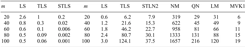
Table I. Left: average relative error of estimation e in per cents as a function ofm. Right: average mega op counts as a function ofm.
m LS TLS STLS m LS TLS STLN2 NM QN LM MVK1
20 2.6 1 0.2 20 0.6 6.2 7.9 319 29 31 6
40 0.8 0.3 0.02 40 1.2 21.6 15.3 622 45 49 9
60 0.6 0.1 0.006 60 1.8 46.2 22.7 958 81 66 11
80 0.5 0.09 0.002 80 2.4 80.7 30.1 1333 131 88 15
[image:14.567.108.448.262.336.2]100 0.5 0.06 0.001 100 3.0 124.1 37.5 1657 216 120 19
Table II. Left: average relative error of estimation e in per cents as a function ofn. Right: average mega op counts as a function ofn.
n LS TLS STLS n LS TLS STLN1 QN LM MVK1
2 1.3 1.3 1.0 2 3 125 167 49 71 21
4 2.3 2.3 1.5 4 8 217 234 127 178 94
8 4.1 4.1 3.1 8 21 421 451 507 619 400
16 5.7 5.4 3.9 16 66 919 750 2235 3021 1446
32 8.9 9.2 5.8 32 219 2355 1877 19568 20643 8478
First we compare the proposed algorithms with the algorithm stln2 from Reference [16] (labelled below STLN2). The structure of the data matrix is Toeplitz withn= 2 andd= 1, i.e. T={[T 3]}, and = 0:015. We use the experiment to show also the asymptotic properties of the estimators. Thus the sample size m is varied from m= 20 to m= 100 with a step of 20 samples.
Table I left shows the average relative error of estimation e= 1=N Nl=1xˆ(l)−x=x in
per cents, where ˆx(l) is the estimate on the lth repetition of the experiment. The various
STLS algorithms have (approximately) equal value of e for all m (in the table the column STLS), which indicates convergence to the same minimum point. Table I right shows the required amount of computations, measured by the average op counts (without those for the computation of the initial approximation). For small n, as in the considered simulation, the most ecient, from the STLS solvers, is the proposed iterative algorithm MVK1, followed by STLN2.
Next we compare the proposed algorithms with the algorithm stln1 from Reference [16] (labelled STLN1). The simulation setup is as the one described above but now the structure is: A Toeplitz, b unstructured, i.e. T={[T n]; [U 1]}, and = 0:05. In this experiment, we x m= 100 and vary n from 2 to 32, in order to illustrate the behaviour of the methods for n=m growing. The NM algorithm is excluded from the comparison because in this experiment its computation is too expensive.
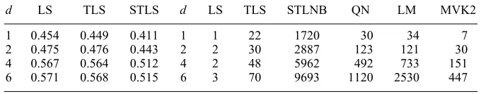
Table III. Left: average relative error of estimation e in per cents as a function ofd. Right: average mega op counts as a function of d.
d LS TLS STLS d LS TLS STLNB QN LM MVK2
1 0.454 0.449 0.411 1 1 22 1720 30 34 7
2 0.475 0.476 0.443 2 2 30 2887 123 121 30
4 0.567 0.564 0.512 4 2 48 5962 492 733 151
6 0.571 0.568 0.515 6 3 70 9693 1120 2530 447
step an unstructured linear system of equations withnequations andnunknowns, which results in computational complexity O(n3). The theoretical computational complexity of STLN1 [15]
is O(n2) in n per iteration.
The last experiment in this subsection deals with a multivariate STLS problem and compares the proposed algorithms with the algorithm of [12] (labelled STLNB). The simulation setup is as described above but the structure of the data matrix is: A Toeplitz with m= 40; n= 2, and B unstructured with d ranging from 1 to 6, i.e. T={[T 2]; [U d]}; = 0:02. The NM algorithm is excluded from the comparison because in this experiment its computation is also too expensive. Table III shows the results. The big dierence between the op counts obtained with STLN1 and STLN2, and those obtained with STLNB is due to the implementation of STLNB, which is not ecient.
6.2. Benchmark test
In Reference [18, Section IV C] an STLS problem with known analytical solution is given. The problem is with n= 1; d= 1, and S( ˆp)—Toeplitz. In this case
ˆ
p(1) pˆ(0) ˆ
p(2) pˆ(1) ..
. ...
ˆ
p(np−1) pˆ(np−2)
S( ˆp)
x
−1
= 0 ⇒ pˆ(l) = ˆp(0)
1 x l
for l= 0; : : : ; np−1
so that the STLS problem
min
x;pˆ p−pˆ 2
2 s:t: S( ˆp)
x
−1
= 0
can be written as
min ;
np−1
l=0
(p(l)−l)2 (17)
where :=p(0) and := 1=x. Eliminating from the rst order optimality condition of (17), the following equation is obtained
H() :=
np−1
l=1
lp(l)l−1
np−1
l=0
2l
−
np−1
l=1
l2l−1
np−1
l=0
p(l)l
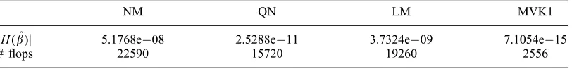
Table IV. Benchmark test.
NM QN LM MVK1
|H( ˆ)| 5.1768e−08 2.5288e−11 3.7324e−09 7.1054e−15
# ops 22590 15720 19260 2556
The left-hand side H() of (18) is a polynomial in of degree 3np−4. The solution ˆ of the STLS problem (17) is the root of H for which the cost function is minimal. The optimal value for is ˆ= np−1
l=0 p(l) ˆl=
np−1
l=0 ˆ2l.
We use equation (18) to check the accuracy of the numerical solutions found by the optimization algorithms. The numerical solutions are computed with the highest possible ac-curacy, i.e. the stopping criterion is x(k−1)−x(k)=x(k−1)¡, where is the machine epsilon.
Table IV shows |H()| when is substituted with the computed STLS solution, and the cor-responding op count. The data for the test isp= [6 5 4 3 2 1] and the initial approximation for the algorithms is the TLS estimate.
The result shows that the MVK1 algorithm achieves better numerical accuracy than the optimization-based algorithms. MVK1 is based on the rst order optimality condition and does not use cost function evaluations. There is a loss of accuracy in the cost function evaluation because the original data C is squared in the computation of f0. Note that the QN method
has 4 more accurate digits than the NM method. This is due to the use of information for the rst derivative in addition to the cost function.
7. CONCLUSIONS
We have proposed ecient numerical methods for the computation of the STLS estima-tor. The structure of the data matrix is specied block-wise, where each of the blocks is Toeplitz=Hankel structured, unstructured, or noise free. The solution methods are based on an equivalent unconstrained optimization problem, in which the correction p is eliminated. The cost function of the equivalent problem is f0(X) =r−1r where the weight matrix
is proportional to the covariance matrix Vr˜ of the centred residual ˜r. Under our structure
assumptions is a block banded Toeplitz matrix.
The proposed numerical methods are (i) standard optimization methods in combination with an ecient cost function and rst derivative evaluation, and (ii) a new iterative method similar to the one proposed in References [19, 20]. Both approaches have computational cost linear in the sample size m. The ecient implementation is possible due to exploitation of the banded structure of the matrix .
ACKNOWLEDGEMENTS
Dr S. Van Huel is a full professor and I. Markovsky is a research assistant at the Katholieke Universiteit Leuven, Belgium. I. Markovsky is supported by a K.U. Leuven doctoral scholarship. Dr A. Kukush is supported by a postdoctoral research fellowship of the Belgian oce for Scien-tic, Technical and Cultural Aairs, promoting Scientic and Technical Collaboration with Central and Eastern Europe. Our research is supported by Research Council KUL: GOA-Mesto 666, IDO=99=003, and IDO=02=009 (predictive computer models for medical classication problems using patient data and expert knowledge), several PhD=postdoc & fellow grants; Flemish Government: FWO: PhD=postdoc grants, projects, G.0200.00 (damage detection in composites by optical bers), G.0078.01 (structured matrices), G.0407.02 (support vector machines), G.0269.02 (magnetic resonance spectroscopic imag-ing), G.0270.02 (non-linear Lp approximation), research communities (ICCoS, ANMMM); AWI: Bil. Int. Collaboration Hungary=Poland; IWT: PhD Grants, Belgian Federal Government: DWTC (IUAP IV-02 (1996-2001) and IUAP V-22 (20IV-02-2006): Dynamical Systems and Control: Computation, Identi-cation & Modelling); EU: NICONET, INTERPRET, PDT-COIL, MRS=MRI signal processing (TMR); Contract Research=agreements: Data4s, IPCOS.
REFERENCES
1. Levin MJ. Estimation of a system pulse transfer function in the presence of noise. IEEE Transactions on Automatic Control 1964;9:229 – 235.
2. Stoica P, Soderstrom T. Bias correction in least-squares identication.International Journal of Control 1982; 35(3):449 – 457.
3. Aoki M, Yue P. Ona priorierror estimates of some identication methods.IEEE Transactions on Automatic Control1970;15(5):541– 548.
4. Golub GH, Van Loan CF. An analysis of the total least squares problem.SIAM Journal on Numerical Analysis
1980;17:883–893.
5. Van Huel S, Vandewalle J.The Total Least Squares Problem:Computational Aspects and Analysis. SIAM: Philadelphia, 1991.
6. Aoki M, Yue P. On certain convergence questions in system identication. SIAM Journal on Control and Optimization 1970;8(2):239 – 256.
7. Kukush A, Markovsky I, Van Huel S. Consistency of the structured total least squares estimator in a multivariate model. Technical Report 02-192, Department EE, K.U. Leuven, 2002.
8. De Moor B. Structured total least squares andL2approximation problems.Linear Algebra and Its Applications
1993;188–189:163– 207.
9. De Moor B, Roorda B.L2-optimal linear system identication structured total least squares for SISO systems.
InThe Proceedings of the Conference on Decision and Control, Peshkin M, McClamroch NH, Yin G (eds), 1994; 2874 – 2879.
10. Gill PE, Murray M, Wright MH.Practical Optimization. Academic Press: New York, 1999.
11. Rosen JB, Park H, Glick J. Total least norm formulation and solution of structured problems.SIAM Journal on Matrix Analysis and Applications 1996;17:1996.
12. Van Huel S, Park H, Rosen JB. Formulation and solution of structured total least norm problems for parameter estimation. IEEE Transactions on Signal Processing1996;44(10):2464 – 2474.
13. Lemmerling P. Structured total least squares: analysis, algorithms and applications.Ph.D. Thesis, ESAT=SISTA, K.U. Leuven, 1999.
14. Mastronardi N. Fast and reliable algorithms for structured total least squares and related matrix problems.Ph.D. Thesis, ESAT=SISTA, K.U. Leuven, 2001.
15. Mastronardi N, Lemmerling P, Van Huel S. Fast structured total least squares algorithm for solving the basic deconvolution problem. SIAM Journal on Matrix Analysis and Applications2000;22:533– 553.
16. Lemmerling P, Mastronardi N, Van Huel S. Fast algorithm for solving the Hankel=Toeplitz structured total least squares problem.Numerical Algorithms 2000;23:371–392.
17. Abatzoglou T, Mendel J, Harada G. The constrained total least squares technique and its application to harmonic superresolution. IEEE Transactions on Signal Processing1991;39:1070 –1087.
18. De Moor B. Total least squares for anely structured matrices and the noisy realization problem. IEEE Transactions on Signal Processing 1994;42(11):3104 –3113.
20. Markovsky I, Rastello M-L, Premoli A, Kukush A, Van Huel S. The element-wise weighted total least squares problem.Technical Report 02 - 48, Department EE, K.U. Leuven, 2002.
21. Nelder JA, Mead R. A simplex method for function minimization.Computer Journal1965;7:308–313. 22. Marquardt D. An algorithm for least squares estimation of non-linear parameters. SIAM Journal on Applied
Mathematics 1963;11:431– 441.
23. Markovsky I, Van Huel S, Kukush A. On the computation of the structured total least squares estimator.
Technical Report 02 - 203, Department EE, K.U. Leuven, 2002.
24. Kukush A, Markovsky I, Van Huel S. About the convergence of the computational algorithm for the EW-TLS estimator. Technical Report 02 - 49, Department EE, K.U. Leuven, 2002.