DEVELOPING A POVERTY MAP OF TAJIKISTAN
A TECHNICAL NOTE
ANGELA BASCHIERI, JANE FALKINGHAM
ABSTRACT
‘Poverty maps’, that is graphic representations of spatially disaggregated estimates of welfare, are being increasingly used to geographically target scare resources. The development of detailed poverty maps in many low resource settings is, however, hampered due to data constraints. Data on income or consumption are often unavailable and, where they are, direct survey estimates for small areas are likely to yield unacceptably large standard errors due to limited sample sizes. Census data offer the required level of coverage but do not generally contain the appropriate information. This has led to the development of a range of alternative methods aimed either at combining survey data with unit record data from the Census to produce estimates of income or expenditure for small areas (Elbers et al. (2002)). This technical note describes the development of a Poverty Map of Tajikistan combining information from the 2003 Tajikistan Living Standards Survey (TLSS) with 2000 Census data. In order to visually present the spatially disaggregated estimates of welfare in Tajikistan, this project has also involved the production of a digital map of the country showing the administrative boundaries at the time of the 2000 Census at both the rayon (district) and jamoat (lowest administrative area) level.
Developing a Poverty Map of Tajikistan
A Technical Note
Angela Baschieri and Jane Falkingham
S3RI Southampton Statistical Sciences Research Institute
Acknowledgements
This work was funded by UK Department for International Development through the World Bank Trust Fund. The development of the Poverty Map of Tajikistan is part of the on-going Poverty Dialogue Program of the World Bank in collaboration with the
Government of Tajikistan. Within the World Bank, the Poverty Dialogue Program is task managed by Dr. Cem Mete.
The authors would sincerely like to thank the Government of Tajikistan for permitting access to the 2000 Census and the 2003 Tajikistan Living Standards Survey. We are indebted to the State Statistical Committee for their invaluable support and collaboration throughout. In particular thanks are due to Prof Mirgand Shabozov (Chairman), Ms. Muhammadieva Bakhtya (First Deputy Chairman), Mr. Khaitov Sulton (Head of Census Division) and Ikhtior Kholmatov (programmer and census data specialist).
Tajikistan Poverty Mapping
1. Introduction
‘Poverty maps’, that is graphic representations of spatially disaggregated estimates of welfare, are being increasingly used to geographically target scare resources. The development of detailed poverty maps in many low resource settings is, however, hampered due to data constraints. Data on income or consumption are often unavailable and, where they are, direct survey estimates for small areas are likely to yield
unacceptably large standard errors due to limited sample sizes. Census data offer the required level of coverage but do not generally contain the appropriate information. This has led to the development of a range of alternative methods aimed either at combining survey data with unit record data from the Census to produce estimates of income or expenditure for small areas (Elbers et al. (2002)). This technical note describes the development of a Poverty Map of Tajikistan combining information from the 2003 Tajikistan Living Standards Survey (TLSS) with 2000 Census data. In order to visually present the spatially disgaggregated estimates of welfare in Tajikistan, this project has also involved the production of a digital map of the country showing the administrative boundaries at the time of the 2000 Census at both the rayon (district) and jamoat (lowest administrative area) level.
2. Overview of the Methodology
spatial autocorrelation in the first stage model and estimating standard errors for the welfare estimates requires additional elaboration.
The method may be thought of being implemented in three. The three stages are preceded by a so called ‘zero stage’. The ‘zero stage’ involves the selection of a set of ‘comparable’ variables common to both the household budget survey and the census. The zero stage is a fundamental part of the success of the poverty mapping procedure as the variables selected in this stage will determined the set of variables to be used for the consumption model, hence the explanatory power of the imputed consumption model. The first stage of analysis then involves the use of survey data to derive a model for predicting household welfare. This model is then applied to the census dataset in the final stage. Stages one and two are further elaborated below.
First Stage
In the “first stage” of analysis a model of consumption is developed using household survey data and those variables that have been selected in the zero stage.
The log of monthly consumption expenditure, is related to a set of observable
characteristics, 1
ch y
ch
x :
[
ch ch]
chch E y x u
y = ln | +
ln (1)
Using a linear approximation, we model the observed log per capita consumption per household h as:
ch ch
ch x u
y = ' β +
ln (2)
where β is a vector of parameters, and u a vector of disturbances, is distributed
. The model (2) is estimated by Generalized Least Squares using data from the
2003 Tajikistan Living Standard Survey. In order to estimate by GLS model, it is first necessary to produce an estimate of
(
0,∑F
)
∑, the associated error covariance matrix. We model individual disturbances as:
ch c ch
u =η +ε
where ηc is a location component and εch is a household component. This error
structure allows for both spatial autocorrelation, i.e. a “location effect” for households in the same area, and heteroskedasticity in the household component of the disturbance. The two components are independent of one another and uncorrelated with observable
characteristics.
In order to estimate∑, we need to calculate the variance of the location component
, the location component
2
η
σ∧ ηc , variance of the household residuals and
household residuals
2 ,ch
ε σ∧
ch
ε 2.
To obtain those parameters we first estimate an OLS regression , and the residuals
from this regression serve as estimates of overall disturbances, given by
.
Wedecompose these into uncorrelated household and location components:
ch
u ∧
ch c
ch e
u = +
∧ ∧
η
where are the within-cluster means of the overall residuals, , household
component estimates are the overall residuals net of location components. ∧
c
η ech
The Elbers et al. (2002) procedure allows for heteroskedasticity in the household
component. In the case of Tajikistan, heteroskedasticity appeared to be significant in some strata; however when we elaborated the so-called alpha model which enables us to capture the heteroskedasticity components, we did not obtain a high R-square. Moreover, as the imputed values were sensitive of the choice of the alpha model regressors, we decided not to estimate the heteroskedasticity component. Given this, we then decided to model only the location component where possible.
Second Stage
In the “second stage” the parameter estimates of the consumption model developed in the first stage are applied to data from the 2000 census of Tajikistan to obtain predicted consumption for each household within the Census.
We construct a series of simulations, where for each simulation r we draw a set of first stage parameters from their corresponding distribution estimated in first stage.
Thus we draw a set of beta and, from the multivariate normal distributions
described by the first stage point estimates and their associated variance–covariance
matrices. Additionally we draw a simulated value of the variance of the location
error component. r ~
β
r ⎟⎟ ⎠ ⎞ ⎜⎜ ⎝ ⎛~2η
σ
For each household we draw simulated disturbance terms, and , from their
corresponding distribution. We simulate a value of expenditure for each household, ,
based on both predicted log expenditure, and their disturbance terms:
. Finally, the full set of simulated per capita consumption
expenditures, are used to calculate the estimate of the welfare measure for each
spatial subgroup. We repeat this procedure 100 times drawing a new , , and
disturbance terms for each simulation. For each subgroup, we take the mean and standard deviation of each welfare measure over 100 simulations.
r
c ~
η rch ~ ε r ch y ∧ r ch x ~ ' β ⎟⎟ ⎠ ⎞ ⎜⎜ ⎝ ⎛ + + = ∧ r ch r c r ch r ch x y ~ ~ ~ '
exp β η ε
r ch y ∧ r ~
α β~r
r ⎟⎟ ⎠ ⎞ ⎜⎜ ⎝ ⎛~2
η
σ
3. The Data
The technique combines the Tajikistan Living Standard Measurement Survey 2003 (TLSS 2003) collected by the State Statistical Committee of Tajikistan, in collaboration with the World Bank, and the 2000 Census of Tajikistan. The Census of Tajikistan covers around 1.6 million households and 6.5 million individuals3. The Republic of Tajikistan is administratively divided in 4 regions: Sodgian oblast, Khatlon oblast,
Gorno-Badagakashan (GBAO), Direct Rule District commonly known as the RRS (Regional Republic Subordination which are 13 autonomous districts) and Dushanbe. There are a total of 58 rayon (districts), 4 districts of Dushanbe, 17 cities subordinated either to the republic or to the oblast. There are 356 jamoat (rural administrative areas) and 13 towns of rural type.
The TLSS 2003 provides information on food consumption, non food consumption, labour activities, agriculture and education. The sampling procedure of the TLSS 2003 allows the estimation of several poverty, education, labour force indicators for the rural and urban areas of the 4 main regions (Sugd, RRS, Khatlon, GBAO) plus Dushanbe. Sugd, Khatlon and GBAO are oblasts subordinate to the Republic, whereas the Republic of Regional Subordination are 13 districts which are directly subordinate to the republic (see Figure 1). However for the TLSS sampling design, the 13 autonomous districts were considered as a separate region. Hence the sampling design incorporates stratification for by region and urban and rural place of residence (9 strata, 4 rural, 5 urban). The sampling has been designed in two stages. In the first stage 208 sampling units representing jamoat were selected. In the second stage a random probability sample of households was drawn from each jamoat using the jamoat household book4. A full list of households was then drawn and a total 4157 households were interviewed5.
3 We consider the de facto population. Retirement homes, the institutional population and the homeless are
excluded from the analysis as those groups were included in the TLSS sample design.
4 The jamoat household book is a book of household information which is administered and updated by
each jamoat office. Its contains demographic, education level and occupation for each household members. It also contains information on household ownership of cattle and possession of land. The book is updated each year and the household book is ‘re-built’ each five years.
5 The actual number of households interviewed were 4160, however after an initial data cleaning 3
Figure 1: Administrative structure of the Republic of Tajikistan as per the census 2000.
Note: the above structure refers to the 2000 census of Tajikistan. It should be noted that several jamoat have been created or merged since 2000 (see appendix C for full list of changes occurred b/w 2000 and 2005).
Sugd Oblast
Khatlon
Oblast GBAO
RRS 13 rayon subordinated to the republic 3 cities subordinated to the republic Dushanbe 14 rayon 8 cities subordinate to the oblast 24 rayon 3 cities subordinated to the rayon 1 cities subordinate to the oblast
7 rayon 1 cities 4 districts 1 Dushanbe city 93 jamoat
4 towns of rural type
130 jamoat
6 towns of rural type
42 jamoat 91 jamoat
3 towns of rural type
Republic of Tajikistan
4. Implementation
Hence, the consumption model was derived using only those variables that were similar both in the wording and distribution across both datasets. In some strata, where the selected variables did not yield a reasonable R square, the criteria for selection of the regression variables were relaxed. From the initial stage of the analysis it became clear that poverty in rural areas was highly related to the environment and that environmental characteristics were a strong predictor of household welfare. To improve the explanatory power of the consumption model was decided to include both census mean variables and some selected environmental variables.
In order to achieve this, it was necessary to construct a digitally referenced map which followed the administrative structure used in the census and which represents the same spatial aggregation of census data. An available jamoat map drawn from the UNDP GIS coordination unit was used and modified according to the census administrative structure. The matching of each polygon in the map and the census territorial code was supervised by Mr Sulton, head of the census at the State Statistical Agency, who was responsible of the implementation of the 2000 Census of Tajikistan6. This facilitated the linking of geographical variables derived from a geo-referenced map to the census dataset.
In order to link both census information and the GIS map to the TLSS, it was also necessary to allocate each primary sampling unit of the survey to a census enumeration area. The household listing of the survey allowed the matching of each primary sampling unit at each settlement area (settlements within each jamoat). The matching of the PSU and census code was completed under the supervision of Mr. Sulton, who was also involved in the TLSS data collection.
Following this, several census mean variables both at settlement level and jamoat level were created and merged with both the TLSS household level data and the census data. In addition several environmental variables were created for each census jamoat area using GIS data on elevation, land cover, and road networks. These were also then linked to both the TLSS and census data sets. Tables 2 and 3 in Appendix A show the list of jamoat and settlement level mean census variables created and Table 4 shows the full
6 The modified census map followed the administrative structure of the republic of Tajikistan at the time of
list of jamoat level GIS variables. All these variables have been tested in the consumption model, but only a subset of these turn out to be significant.
A separate consumption model was estimated for each strata using the variables selected in the ‘zero stage’ within each strata. We then estimated the location effect, and regressed the jamoat or settlement area variables (derived either from the census data or GIS maps) to identify a subset of variables which acted to reduce this effect. The consumption model within each strata was then re-estimated, including those spatial (locational) variables which were significant at 1 % level. In few cases, we also included variables which were significant at 5 or 10 per cent level in order to increase the R square; this was particularly the case in rural areas (see Table 5 and 6 Appendix A).
The results of the OLS regressions in Tables 5 and 6 in Appendix A show that the regression models were quite successful in explaining the variation in monthly
consumption expenditure in urban areas, with R-square values ranging from 26 per cent to 50 per cent. The models were less well specified in rural areas, where the R-square values range from 20 per cent to 31 per cent. This is mainly due to the fact that consumption expenditure is highly related to the characteristics of the environment of where people live. The R square of the consumption models in rural areas was even lower without the inclusion of GIS variables.
The parameters estimates derived in the first stage modelling, were then applied to the census data to impute consumption expenditure using the methodology described above. In order to derive community estimates of headcount poverty, two alternative poverty lines were employed a) an absolute poverty line of 47.06 Somoni per month, and b) a relative poverty line of the bottom 40% percentile (corresponding to 33.37 Somoni per month).
5. Results
Table 1 below presents the results for the monthly consumption expenditure
model appears to work quite well for the estimation of the mean monthly consumption
expenditure adjusted for regional prices. However, looking at the GINI coefficient and FGT(1), there appears to be much lower degree of correspondence between the two data sources. Thus it appears that the consumption model performs less well in predicting the
distribution of the monthly consumption expenditure. This is not usual as the imputation
process is less able to replicate the outliers that occur in real life.
[image:12.612.100.564.320.618.2]The imputed values for the proportion of people living in a household with a consumption expenditure below the absolute poverty line of 47.06 Somoni are more robust for urban areas than for rural areas, whereas the opposite is true for the imputation of the proportions of people living in relative poverty.
Table 1: Poverty and Inequalities in Tajikistan, by oblast (strata).
Mean FTG(0) FGT(1) FTG(0) GINI
PL=47.06 S PL=33.37 S
Census TLSS Census TLSS Census TLSS Census TLSS Census TLSS
Urban
Gbao 39.31 40.38 0.721 0.739 0.277 0.253 0.466 0.407 0.283 0.260
(1.39) (1.86) (0.025) (0.039) (0.016) (0.023) (0.025) (0.049) (0.014) (0.019)
Sugd 49.52 50.03 0.610 0.586 0.245 0.218 0.405 0.364 0.366 0.339
(1.43) (1.85) (0.016) (0.027) (0.011) (0.014) (0.016) (0.027) (0.010) (0.014)
Khatlon 36.71 37.02 0.761 0.775 0.376 0.348 0.587 0.611 0.396 0.346
(1.59) (1.78) (0.018) (0.028) (0.015) (0.019) (0.020) (0.035) (0.022) (0.018)
Dushanbe 56.04 59.11 0.531 0.489 0.199 0.165 0.328 0.268 0.364 0.349
(1.44) (1.72) (0.017) (0.022) (0.011) (0.011) (0.016) (0.021) (0.007) (0.009)
RRS 57.47 52.06 0.581 0.552 0.203 0.168 0.342 0.282 0.332 0.290
(2.57) (2.72) (0.030) (0.050) (0.019) (0.020) (0.033) (0.050) (0.028) (0.022)
Rural
Gbao 33.70 32.59 0.791 0.858 0.393 0.373 0.616 0.626 0.369 0.290
(1.51) (1.01) (0.022) (0.018) (0.011) (0.013) (0.019) (0.026) (0.023) (0.012)
Sugd 46.80 45.1 0.620 0.663 0.222 0.223 0.373 0.368 0.307 0.288
(1.17) (0.93) (0.013) (0.017) (0.007) (0.008) (0.012) (0.018) (0.010) (0.007)
Khatlon 39.22 40.02 0.731 0.782 0.312 0.304 0.519 0.525 0.332 0.323
(1.33) (1.08) (0.018) (0.014) (0.014) (0.008) (0.020) (0.018) (0.011) (0.012)
RRS 60.66 56.54 0.457 0.436 0.154 0.135 0.251 0.214 0.335 0.279
(1.83) (1.25) (0.016) (0.022) (0.009) (0.009) (0.014) (0.019 (0.012) (0.008)
(districts) by the coefficient of variation. Considering the coefficient of variation derived by the survey stratum estimate as a cut off point for the level of acceptable error, we can see that around 90 per cent of the estimates of mean consumption expenditure are below the coefficient of variation obtained from the survey. Good results are also shown for the rayon estimates of FGT(0), FGT(1) and GINI (figures B2, B3 and B4). Jamoat level estimates confirm the results obtained at the rayon level; around 80 per cent of those estimates are below the coefficient of variation for both the monthly consumption expenditure and the headcount rate (figures B5-B8). However for the urban areas, the estimates appear not to be robust for half of the cities (figures B9-B12). However, it should be noted that the urban areas include both ‘cities subordinate to the oblast’, which are generally large in size, and ‘settlements of urban type which are subordinate to the rayon’, which are much smaller in size. Disaggregating these, the results appear to be more stable for bigger cities.
The standard errors associated with those estimates do not account for possible errors due to the misspecification of the model we have used for the imputation in the census. Although the procedure technically allows estimating welfare indicators for low levels of disaggregation, the model errors associated with estimates based on areas containing below 1000 households are felt to be too high to be reliable. These problems particularly affect the jamoat level estimates in GBAO and in Tavildara Rayon where the there are frequently less than a 1,000 households within each jamoat (at the time of the 2000 Census).
the 2003 survey. Given that the "zero" stage exercise ensured that only variables with the same meaning and distribution across the two datasets were selected for the regression, it made be inferred that the procedure is imputing 2003 consumption into the 2000 census. Thus the map can be argued to be presenting a picture of the 2003 spatial distribution of poverty.
In reality the map presents a picture of poverty in neither 2000 or 2003. During the period between the census and the survey there have been both economic growth and extensive migration. Hence both the imputed welfare regression (which comes form the household budget) and the spatial distribution of the population (which comes from the census) are likely to have changed between the two years. Thus it is best to interpret the map as providing a guide to the spatial distribution of welfare at the start of the twenty-first century i.e. over the period 2000-2003.
5.1 The spatial distribution of poverty
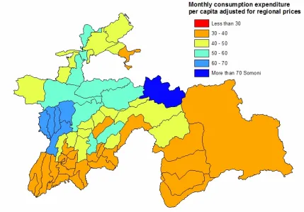
Bearing these caveats in mind, Figure 1 presents the jamoat level estimates of the monthly consumption expenditure for the country. Areas with less than 1,000 households are shaded to indicate their potential unreliability. The poorest region of the country is Khatlon oblast, where the majority of jamoats have a mean per capita monthly
consumption expenditure of less than 40 Somoni. There are also clusters of poverty in Isfara, Roguum, Darvuz and Panjekent. Several district in RRS (Vahdat, Varzob, Rudaki, Tursanzoda, Jirgatol, ect.) and Ghafurov and Matchin districts in Sogd, and Vanj rayon in GBAO show the highest level of monthly consumption expenditure.
Using the same right hand side variables, the consumption model was re-estimated to impute monthly consumption expenditure not adjusting for regional prices, monthly food consumption and monthly food consumption expenditure not adjusting for regional prices. The results are shown in Figures 2-4 respectively.
Figure 1: Monthly consumption expenditure per capita adjusted for regional prices
[image:15.612.92.484.429.711.2]Figure 3 below shows the poverty map for the monthly food consumption expenditures. Using this measure as our welfare indicator modifies the picture somewhat. However, the jamoat in Khatlon again appear again at the bottom of the ranking, whereas the jamoat in RRS area again appears at the top end. Interesting if we do not adjust for regional prices, the monthly food consumption expenditure map changes, and some jamoat change their ranking. This is especially true for rayon in Sugd (Figure 4).
Figure 4: Monthly food consumption expenditure not adjusted for regional prices
Figure 5: Proportion of people with a consumption expenditure below the absolute poverty line of 47.06 Somoni
[image:18.612.92.475.408.705.2]Figure 7: Proportion of people with a monthly food consumption expenditure below the relative poverty line of the 40th percentile (21.95 Somoni).
5.2 What have we learnt by increasing disaggregation?
Figure 8: Rayon map of consumption expenditure adjusted for regional prices
Figure C1- C6 in Appendix C shows the spatial heterogeneity of poverty at both the rayon and jamoat level for urban and rural areas. The graphs compare the estimates and their associated confidence intervals with the national value. Looking at Figures C4 and C5, we can see that spatial inequalities increase by moving from rayon level estimates to jamoat level estimates. Moreover, the graphs illustrate that using a national average masks considerable spatial heterogeneity with some rayons and jamoats experience headcount poverty rates well above the national estimate for rural areas.
5.3 Poverty and Inequalities in urban areas
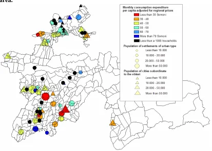
Figures 9 and 10 show the estimates for mean monthly per capita consumption expenditure in urban areas. As discussed above, there are two types of urban areas – ‘cities subordinate to the oblast’ and ‘settlements of urban types’. The results for urban areas show higher rates of poverty in urban area of Khatlon and high inequalities in
Figure 9: Monthly consumption expenditure adjusted for regional prices, urban area.
[image:21.612.92.499.424.703.2]6. Summary
By combining information from the 2003 Tajikistan Living Standards Survey and the 2000 Census it is possible to produce spatially disaggregated estimates of welfare based on consumption at the sub-oblast level. The key findings are:
¾
In general, there is a higher incidence of both absolute and relative poverty in rural areas as compared to urban areas.¾
However, there is a high degree of variation in poverty across urban areas, with the proportion of the population living below the absolute poverty line varying between 10 and 95 per cent.¾
There is also a significant degree of variation within rayons, with somepockets of deprivation within more affluent areas.
¾
Overall, poverty rates appear to be highest in Khatlon and GBAO and lowest in RRS, which is consistent with the World Bank Poverty assessement.¾
Comparing the spatial estimates of welfare derived using per capita consumption with and without regional price adjustments highlights that although absolute levels are sensitive to price adjustments, the relative ranking of jamoats is fairly robust.It is important to note that the spatially disaggregated estimates of welfare presented here should be interpreted with caution both in terms of the robustness of the imputation model and the size of the standard errors around the point estimates. These concerns need to be borne in mind particularly when using poverty maps for geographical targeting, and it is preferable for such maps to be employed in conjunction with other targeting
Appendix A
Table 1: Descriptive statistics, urban and rural areas.
GBAO Urban Sugd Urban Khatlon Urban
GBAO Urban Sugd Urban Khatlon Urban
Census 2000 TLSS 2003 l95b u95b Census 2000 TLSS 2003 l95b u95b Census 2000 TLSS 2003 l95b u95b hh_sec 0.644 0.458 0.519 0.616 0 0.591 0.568 0.519 0.616 1 0.661 0.536 0.470 0.601 0 hh_high 0.271 0.433 0.347 0.523 0 0.202 0.303 0.260 0.350 0 0.195 0.245 0.193 0.306 1 prnone 0.100 0.182 0.151 0.213 0 0.125 0.201 0.178 0.223 0 0.144 0.323 0.293 0.352 0 proppri 0.175 0.121 0.095 0.148 0 0.220 0.104 0.087 0.120 0 0.216 0.166 0.142 0.189 0 propsec 0.463 0.488 0.442 0.534 1 0.429 0.556 0.528 0.585 0 0.396 0.428 0.397 0.458 0 prophigh 0.167 0.207 0.172 0.241 0 0.117 0.137 0.116 0.156 1 0.073 0.082 0.064 0.101 1 hh_be15 0.005 0.000 0 0 0 0.007 0.000 0.000 0.000 0 0.002 0.000 0.000 0.000 0 hh_1560 0.776 0.675 0.586 0.752 0 0.784 0.754 0.709 0.794 1 0.817 0.736 0.674 0.790 0 hh_ab60 0.219 0.325 0.247 0.413 0 0.209 0.245 0.205 0.290 1 0.181 0.263 0.209 0.325 0 prop15 0.287 0.228 0.195 0.261 0 0.285 0.287 0.266 0.309 1 0.406 0.401 0.371 0.431 1 prop1560 0.648 0.678 0.637 0.718 1 0.608 0.590 0.564 0.617 1 0.531 0.528 0.500 0.556 1 propab60 0.065 0.093 0.061 0.125 1 0.107 0.121 0.095 0.147 1 0.063 0.070 0.049 0.090 1 tthh4 0.481 0.375 0.266 0.483 1 0.570 0.453 0.383 0.523 0 0.888 0.763 0.640 0.886 1 tthh5_7 0.032 0.241 0.155 0.328 1 0.320 0.288 0.231 0.345 1 0.526 0.554 0.461 0.647 1 tthh8_14 0.915 0.758 0.605 0.911 1 0.830 0.857 0.765 0.949 1 1.193 1.177 1.030 1.323 1 tthh15_4 1.262 1.350 1.120 1.570 1 1.066 1.072 0.947 1.197 1 1.043 1.113 0.937 1.289 1 tthh25_4 1.872 1.810 1.568 2.060 1 1.479 1.318 1.219 1.417 0 1.536 1.586 1.460 1.712 1 tthh45_6 0.600 0.850 0.702 0.997 0 0.491 0.556 0.480 0.632 1 0.423 0.427 0.339 0.515 1 tthh60 0.329 0.466 0.351 0.582 1 0.340 0.338 0.280 0.396 1 0.248 0.318 0.241 0.394 1
Obs 4950 120 24 124305 399 22 65657 220 24 N of rayon ** ** ** ** ** ** N of city sub 1 1 8(6+1(2)+1(7)) 7(5+1+1(2)) 4 3 N city in rayon 0 0 15 4 20 5 N jamoat ** ** ** ** ** ** N town (rur) ** ** ** ** ** ** N of settlements ** ** ** ** ** **
Table 1: Descriptive statistics, urban and rural areas, continued.
Dushanbe RRS Urban GBAO Rural
Census 2000 TLSS 2003 l95b u95b Census 2000 TLSS 2003 l95b u95b Census 2000 TLSS 2003 l95b u95b
Dushanbe RRS Urban GBAO Rural
Census 2000 TLSS 2003 l95b u95b Census 2000 TLSS 2003 l95b u95b Census 2000 TLSS 2003 l95b u95b
hh_high 0.314 0.428 0.391 0.466 0 0.159 0.158 0.103 0.235 1 0.189 0.297 0.252 0.346 0 prnone 0.090 0.221 0.203 0.239 0 0.118 0.314 0.272 0.357 0 0.122 0.256 0.234 0.277 0 proppri 0.173 0.103 0.091 0.115 0 0.261 0.186 0.148 0.223 0 0.244 0.139 0.123 0.154 0 propsec 0.430 0.448 0.424 0.472 1 0.402 0.445 0.399 0.490 1 0.429 0.527 0.502 0.552 0 prophigh 0.188 0.223 0.201 0.245 0 0.071 0.053 0.029 0.077 1 0.064 0.077 0.063 0.090 1 hh_be15 0.004 0.000 0.000 0.000 0 0.006 0.000 0.000 0.000 0 0.001 0.000 0.000 0.000 0 hh_1560 0.850 0.802 0.770 0.831 0 0.822 0.783 0.700 0.848 1 0.736 0.711 0.662 0.755 1 hh_ab60 0.146 0.197 0.168 0.229 0 0.172 0.216 0.152 0.299 1 0.263 0.288 0.244 0.337 1 prop15 0.275 0.309 0.290 0.328 0 0.373 0.357 0.315 0.399 1 0.373 0.331 0.308 0.354 0 prop1560 0.644 0.579 0.557 0.601 0 0.551 0.563 0.518 0.609 1 0.547 0.574 0.551 0.597 0 propab60 0.081 0.111 0.090 0.132 1 0.076 0.078 0.043 0.114 1 0.080 0.094 0.075 0.112 1 tthh4 0.569 0.562 0.539 0.877 1 0.772 0.708 0.539 0.877 1 0.837 0.622 0.534 0.709 0 tthh5_7 0.315 0.352 0.307 0.397 1 0.472 0.391 0.290 0.493 1 0.525 0.475 0.407 0.542 1 tthh8_14 0.721 0.820 0.741 0.899 0 1.148 1.183 0.981 1.384 1 1.339 1.060 0.957 1.176 0 tthh15_4 2.022 0.875 0.785 0.965 0 1.211 1.110 0.901 1.332 1 1.459 1.466 1.311 1.622 1 tthh25_4 1.295 1.290 1.220 1.368 1 1.590 1.400 1.195 1.604 1 1.828 1.733 1.617 1.849 1 tthh45_6 0.350 0.430 0.380 0.482 0 0.422 0.575 0.444 0.705 0 0.564 0.597 0.517 0.677 1 tthh60 0.209 0.262 0.220 0.305 0 0.280 0.291 0.187 0.396 1 0.452 0.455 0.386 0.524 1
Obs 140769 658 12 33145 120 28 26414 360 21 N of rayon ** ** ** ** 7 7 N of city sub 4 4 3 2 ** ** N city in rayon 10 2 ** N jamoat ** ** ** ** 42 18 N town (rur) ** ** ** ** 0 0 N of settlements ** ** ** ** 395 **
Table 1: Descriptive statistics, urban and rural areas, continued.
Sugd Rural Khatlon Rural RRS Rural
Census 2000 TLSS
2003
l95b u95b Census 2000 TLSS 2003 l95b u95b Census 2000 TLSS 2003 l95b u95b
hh_size 6.515 6.217 6.025 6.409 0 7.840 7.322 7.125 7.519 0 8.057 8.031 7.731 8.330 1 hh_work 0.710 0.681 0.650 0.712 1 0.748 0.706 0.674 0.736 0 0.677 0.591 0.551 0.631 0 hh_marr 0.834 0.805 0.776 0.829 0 0.853 0.854 0.828 0.876 1 0.825 0.816 0.782 0.845 1 hh_di_se 0.013 0.015 0.008 0.026 0 0.011 0.003 0.001 0.011 1 0.014 0.008 0.004 0.021 1 hh_widow 0.142 0.165 0.142 0.192 1 0.121 0.138 0.116 0.163 1 0.144 0.159 0.131 0.191 1 hh_fem 0.139 0.152 0.129 0.178 1 0.117 0.126 0.105 0.150 1 0.144 0.156 0.129 0.188 1 sephouse 0.829 0.920 0.900 0.940 0 0.924 0.930 0.910 0.950 1 0.811 0.930 0.900 0.950 0 shahouse 0.139 0.064 0.049 0.082 0 0.059 0.049 0.036 0.066 1 0.165 0.022 0.013 0.038 0 sepapart 0.016 0.006 0.002 0.014 0 0.007 0.005 0.002 0.013 0 0.014 0.036 0.024 0.055 0 shaapart 0.002 0.000 0.000 0.000 0 0.007 0.000 0.000 0.000 0 0.006 0.000 0.000 0.000 0 dwebef60 0.111 0.119 0.099 0.142 1 0.095 0.079 0.062 0.099 1 0.122 0.105 0.083 0.133 1 dwe60_80 0.372 0.407 0.375 0.440 0 0.425 0.366 0.334 0.399 0 0.414 0.512 0.471 0.553 0 dwe80_90 0.255 0.243 0.216 0.273 1 0.248 0.304 0.273 0.336 0 0.242 0.288 0.253 0.326 0 dweaft90 0.157 0.231 0.204 0.261 0 0.183 0.252 0.224 0.283 0 0.109 0.095 0.074 0.122 1 eleoven 0.009 0.197 0.171 0.224 0 0.033 0.218 0.191 0.247 0 0.144 0.312 0.276 0.351 0 stooven 0.641 0.705 0.673 0.734 0 0.933 0.914 0.893 0.931 0 0.808 0.888 0.860 0.911 0 waterpip 0.043 0.137 0.116 0.162 0 0.074 0.262 0.233 0.293 0 0.200 0.364 0.326 0.404 0 telep 0.024 0.051 0.038 0.068 0 0.007 0.008 0.004 0.017 0 0.011 0.053 0.038 0.075 0 owndwe 0.971 0.972 0.959 0.981 1 0.979 0.862 0.947 0.973 0 0.978 0.935 0.911 0.952 0 areles 0.210 0.221 0.194 0.250 1 0.113 0.166 0.142 0.192 0 0.141 0.062 0.045 0.085 1 area40_69 0.389 0.399 0.367 0.432 1 0.365 0.488 0.454 0.522 0 0.292 0.357 0.319 0.397 0 areamo70 0.401 0.379 0.347 0.412 1 0.521 0.344 0.313 0.377 0 0.567 0.576 0.535 0.616 1 cenheat 0.022 0.000 0.000 0.000 0 0.007 0.000 0.000 0.000 0 0.013 0.029 0.018 0.047 0 numroom 2.830 3.809 3.759 3.858 0 3.600 3.222 3.130 3.314 0 3.574 3.763 3.699 3.827 0 prwork 0.377 0.346 0.332 0.361 0 0.378 0.337 0.325 0.349 0 0.346 0.357 0.337 0.377 1 hh_none 0.057 0.092 0.074 0.113 0 0.025 0.092 0.074 0.113 0 0.040 0.167 0.139 0.199 0
Sugd Rural Khatlon Rural RRS Rural
Census 2000 TLSS
2003
l95b u95b Census 2000 TLSS 2003 l95b u95b Census 2000 TLSS 2003 l95b u95b
hh_high 0.125 0.212 0.186 0.241 0 0.112 0.166 0.143 0.193 0 0.105 0.210 0.179 0.245 0 prnone 0.165 0.251 0.237 0.265 0 0.162 0.336 0.322 0.350 0 0.134 0.318 0.302 0.334 0 proppri 0.233 0.116 0.106 0.127 0 0.245 0.158 0.146 0.169 0 0.295 0.162 0.150 0.175 0 propsec 0.400 0.563 0.546 0.580 0 0.368 0.469 0.454 0.484 0 0.364 0.465 0.448 0.482 0 prophigh 0.044 0.067 0.058 0.077 0 0.027 0.036 0.030 0.041 0 0.031 0.052 0.004 0.061 0 hh_be15 0.004 0.000 0.000 0.000 0 0.001 0.000 0.000 0.000 0 0.003 0.000 0.000 0.000 0 hh_1560 0.768 0.754 0.724 0.782 1 0.782 0.751 0.720 0.779 0 0.756 0.684 0.645 0.721 0 hh_ab60 0.229 0.245 0.217 0.275 1 0.218 0.248 0.220 0.279 0 0.242 0.316 0.279 0.355 0 prop15 0.385 0.343 0.330 0.357 0 0.458 0.415 0.401 0.428 0 0.427 0.376 0.360 0.392 0 prop1560 0.538 0.569 0.554 0.585 0 0.482 0.521 0.508 0.534 0 0.505 0.543 0.526 0.559 0 propab60 0.077 0.086 0.073 0.099 1 0.059 0.063 0.054 0.072 1 0.068 0.080 0.067 0.093 0 tthh4 0.917 0.783 0.714 0.852 0 1.297 1.000 0.933 1.083 0 1.237 1.081 0.984 1.178 0 tthh5_7 0.516 0.472 0.428 0.515 1 0.755 0.585 0.540 0.631 0 0.707 0.607 0.542 0.672 0 tthh8_14 1.204 0.998 0.928 1.069 0 1.621 1.516 1.434 1.598 0 1.615 1.499 1.388 1.601 0 tthh15_4 1.294 1.367 1.270 1.463 1 1.484 1.651 1.544 1.757 0 1.663 1.893 1.762 2.024 0 tthh25_4 1.709 1.627 1.553 1.702 1 1.813 1.569 1.498 1.640 0 1.887 1.821 1.712 1.929 1 tthh45_6 0.490 0.603 0.549 0.657 0 0.496 0.617 0.562 0.671 0 0.520 0.644 0.581 0.707 0 tthh60 0.385 0.363 0.322 0.405 1 0.374 0.375 0.331 0.418 1 0.429 0.489 0.432 0.546 0 Obs 249624 860 17 241347 840 10 172063 580 11
N of rayon 14 13 24 21 13 12 N of city sub ** ** ** ** ** ** N city in rayon ** ** ** ** N jamoat 93 43 130 38 91 27 N town (rur) 4 0 6 4 3 1 N of
settlements
654 ** 1528 ** 1225
Table 2: Census derived Jamoat level mean variables tested in the model.
VARIABLE NAME Variables label
jamoat Jamoat code
jamopop Total population in each jamoat jamohh Total number of hh in each jamoat tot5 Total number of person 5 or less years old tot6_10 Total number 6 to 10 years old
tot11_15 Total number 11 to 15 years old tot16_20 Total number 16 to 20 years old tot21_25 Total number 21 to 25 years old tot26_30 Total number 26 to 30 years old tot31_35 Total number 31 to 35 years old tot36_40 Total number 36 to 40 years old tot41_45 Total number 41 to 45 years old tot46_50 Total number 45 to 50 years old tot51_55 Total number 51 to 55 years old tot56_60 Total number 56 to 60 years old tot61_65 Total number 61 to 65 years old totab65 Total number above 65 years old illiterate Proportion 17 old illiterate
primary Proportion 17 old with primary education secondary Proportion 17 old with secondary education higher Proportion 17 old with higher education active Proportion of 15 years old economically active indibasi proportion of 15 old working on individual basic employee proportion of 15 old working on working as an employee
Source1 prop of 15 yrs old working as an employee at an enterprise or in organization or in institution Source2 prop of 15 yrs old working as an employee at dekhkan farm
[image:29.612.84.524.85.375.2]Source8 prop of 15 yrs old working one ancillary farm Source10 Proportion of pensioner
Table 3: Census derived settlement level mean variables tested in the model.
VARIABLES NAME Variables label
prsephh proportion of hh living in a separate hh per village prshahh proportion of hh living in a share hh per village prsaphh proportion of hh living in a sep apart hh per village prshaph proportion of hh living in a share apart hh per village Prbe60hh prop of hh living in a house built bef 60 per village prdw68hh prop of hh living in a house built 60_80 per village prdw89hh prop of hh living in a house built 80_90 per village prdaf90h prop of hh living in a house built aft 90 per village prelepvh prop of hh living in hh which have electric oven prstovhh prop of hh living in hh which stone oven prwatpih prop of hh living in hh which water pipes prtelehh prop of hh living in hh which telep prownhh prop of hh living in hh which own d avnuroom average num room per hh in village
prarlesh prop of hh living in hh which has a living area less than 40 m prar4_8h prop of hh living in hh which has a living area b 40 69 m2 prarmo7h prop of hh living in hh which has a living area more than 70 m prhh_mar prop of hh head married per village
prhh_ds prop of hh head divorced/separated per village prhh_wi prop of hh head widow per village
prhh_fem prop of hh head female per village prhh_wor prop of hh head work per village prhh_no prop of hh head none education per village prhh_pri prop of hh head primary education per village prhh_sec prop of hh head secondary education per village prhh_hig prop of hh head higher education per village prhh_b15 prop of hh head below 15 per village prhh_156 prop of hh head below 15/60 per village prhh_a60 prop of hh head below above60 per village avhh_siz average num room per hh in village avtoarea Average living area
tpri proportion of village members with primary education tsec proportion of village members with secondary education thigh proportion of village members with higher education prwork proportion of village members economically active prbe15 proportion of village members below 15 years old pr1560 proportion of village members below 15/60 prab60 proportion of village members above 60
prentorg prop of village members employed in enterprise organization or institution prdenkha prop of village members employed in dekhkan farm
prindcit
prowndek prop of village members employed own denkhan prowpr prop of village members employed own private enterprise prind prop of village members employed individual basis prfament prop of village members employed family enterprise prancfar prop of village members employed at one's own ancillary farm prpensi prop of village members employed living from pension prumplbe unemployment benefit
[image:30.612.93.526.260.712.2]prbenef other benefit/gov support
Table 4: GIS variables at jamoat level tested in the model.
VARIABLE NAME label
aveheig2 Average height, buffer for settlements 200
lan0_202 Proportion of land between 0-5 ° slope, buffer for settlement 200 ln5_202 Proportion of land between 5_20 ° slope, buffer for settlement 200 lnab202 Proportion of land above 20 ° slope, buffer for settlement 200
aveheig5 Average height, buffer for settlements 200
lan0_205 Proportion of land between 0-5 ° slope, buffer for settlement 500 ln5_205 Proportion of land between 5_20 ° slope, buffer for settlement 500 lnab205 Proportion of land above 20 ° slope, buffer for settlement 500
aveheig1 Average height, buffer for settlements 200
lan0_201 Proportion of land between 0-5 ° slope, buffer for settlement 1000 ln5_201 Proportion of land between 5_20 ° slope, buffer for settlement 1000 lnab201 Proportion of land above 20 ° slope, buffer for settlement 1000
aveheigk Average height, buffer for settlements 200
lan0_20k Proportion of land between 0-5 ° slope, buffer for settlement 1500 ln5_20k Proportion of land between 5_20 ° slope, buffer for settlement 1500 lnab20k Proportion of land above 20 ° slope, buffer for settlement 1500
avedist Average distance to road
cr_oth15 Prop of cropland, ‘other’ cat within jamoat or 1,5k buffer around set
cr_unk15 Prop of cropland, ‘unknown’ cat within jamoat or 1,5k buffer around settlement (might correspond to cotton)
cr_dry15 Prop of cropland, ‘dry’ category within jamoat or 1,5k buffer around set gr_gra15 Prop of grassland, ‘grass’ cat within jamoat or 1,5k buffer around set gr_scr15 Prop of grassland, ‘scrub’ cat within jamoat or 1,5k buffer around set tundra15 Prop of tundra within jamoat or 1,5k buffer around set
tr_eve15 Prop of trees, ‘evergreen’ cat within jamoat or 1,5k buffer around set tr_mix15 Prop of trees, ‘mixed’ cat within jamoat or 1,5k buffer around set tr_dec15 Prop of trees land, ‘deciduous’ cat within jamoat or 1,5k buffer around set
cr_oth1 Prop of cropland, ‘other’ cat within jamoat or 1k buffer around set
cr_unk1 Prop of cropland, ‘unknown’ cat within jamoat or 1k buffer around settlement (might correspond to cotton)
cr_dry1 Prop of cropland, ‘dry’ category within jamoat or 1k buffer around set gr_gra1 Prop of grassland, ‘grass’ cat within jamoat or 1k buffer around set gr_scr1 Prop of grassland, ‘scrub’ cat within jamoat or 1k buffer around set tundra1 Prop of tundra within jamoat or 1k buffer around set
tr_eve1 Prop of trees, ‘evergreen’ cat within jamoat or 1k buffer around set tr_mix1 Prop of trees, ‘mixed’ cat within jamoat or 1k buffer around set tr_dec1 Prop of trees land, ‘deciduous’ cat within jamoat or 1k buffer around set
cr_unk5 Prop of cropland, ‘unknown’ cat within jamoat or 0,5k buffer around settlement (might correspond to cotton)
cr_dry5 Prop of cropland, ‘dry’ category within jamoat or 0,5k buffer around set gr_gra5 Prop of grassland, ‘grass’ cat within jamoat or 0,5k buffer around set gr_scr5 Prop of grassland, ‘scrub’ cat within jamoat or 0,5k buffer around set Tundra5 Prop of tundra within jamoat or 0,5k buffer around set
tr_eve5 Prop of trees, ‘evergreen’ cat within jamoat or 0,5k buffer around set tr_mix5 Prop of trees, ‘mixed’ cat within jamoat or 0,5k buffer around set tr_dec5 Prop of trees land, ‘deciduous’ cat within jamoat or 0,5k buffer around set
cr_oth2 Prop of cropland, ‘other’ cat within jamoat or 0,2 k buffer around set
cr_unk2 Prop of cropland, ‘unknown’ cat within jamoat or 0,2 k buffer around settlement (might correspond to cotton)
cr_dry2 Prop of cropland, ‘dry’ category within jamoat or 0,2 k buffer around set gr_gra2 Prop of grassland, ‘grass’ cat within jamoat or 0,2 k buffer around set gr_scr2 Prop of grassland, ‘scrub’ cat within jamoat or 0,2 k buffer around set Tundra2 Prop of tundra within jamoat or 0,2 k buffer around set
Table 5: OLS regression for the urban strata.
Urban strata: GBAO Sugd Khatlon Dushanbe RRS
Demographic variables
hh_size -0.091 0.003
(7.84)*** (0.16)
tthh4 -0.154 -0.089 -0.180
(2.61)** (3.64)*** (4.27)***
tthh5_7 -0.139
(1.94)*
tthh8_14 -0.129
(3.23)***
tthh15_4 -0.101 -0.118
(3.77)*** (2.49)**
tthh25_4 -0.097 0.033
(3.87)*** (0.69)
sqth25_4 -0.022
(2.34)**
tthh60 -0.152
(1.91)*
hh_fem 0.179
(2.01)**
prop1560 0.331
(2.58)**
prop15 -0.761 0.366
(2.65)*** (1.76)*
Socio-economic variables
hh_pri -0.371
(2.74)***
hh_sec 0.167
(2.03)**
propsec -0.612
(3.92)***
hh_work 0.133
(2.32)**
prwork 0.833 0.385
(6.61)*** (2.13)**
prophigh 0.868 1.004 0.637 1.456
(5.50)*** (3.41)*** (5.67)*** (4.09)***
Household characteristics
dwe80_90 -0.181
(2.06)**
stooven -0.234 0.112
(3.15)*** (1.89)*
are40_69 0.131 -0.164 -0.153
(1.91)* (2.54)** (2.06)**
aremo70 0.144
(2.13)**
sepapart 0.327
(3.03)***
dweaft90 0.331
(2.08)**
areles -0.162 -0.296
(1.83)* (4.31)***
Urban strata: GBAO Sugd Khatlon Dushanbe RRS
active -18.555 4.155
(1.87)* (2.97)***
indibasi 19.805 -3.336
(1.86)* (2.34)**
employee 22.055
(1.86)*
source1 -4.103
(2.47)**
source8 15.975
(2.18)**
prstovhh 3.038 0.772
(4.34)*** (3.12)***
prdw89hh 1.262
(2.20)**
prtelehh 1.453
(1.90)*
prwatpih 0.793
(2.86)***
avnuroom -1.299
(3.46)***
prarlesh 6.695
(4.84)***
prhh_mar 10.462
(3.96)***
Constant 4.614 3.813 -4.039 2.776 2.912
(34.60)*** (9.45)*** (2.12)** (6.72)*** (15.25)***
Observations 120 399 220 658 120
R-squared 0.50 0.28 0.33 0.26 0.43
Absolute value of t statistics in parentheses
Table 6: OLS regression for the rural strata.
Rural strata: Gbao Sugd Khatlon RRS
Demographic variables
hh_size -0.101 -0.107 -0.116
(5.88)*** (5.21)*** (6.78)***
hhsize2 0.003 0.003 0.004
(3.35)*** (2.80)*** (5.77)***
tthh5_7 -0.054 (1.51) tthh15_4 -0.076 (4.51)*** tthh25_4 -0.093 (4.30)*** tthh60 -0.183 (2.86)***
prop1560 0.285
(3.20)***
propab60 0.551 0.302
(1.64) (2.07)**
hh_1560 -0.153
(1.91)*
hh_fem -0.150
(3.15)***
hh_marr 0.143
(2.61)***
Socio economic variables
hh_sec -0.137
(3.90)***
prophigh 0.898
(3.98)***
Household characteristics
are40_69 0.114
(2.38)**
aremo70 0.231 0.150
(4.74)*** (3.23)***
stooven -0.174
(3.05)***
owndwe 0.269
(2.88)***
Census mean variables
prsephh -1.874
(4.40)***
avnuroom -0.386 0.054
(4.20)*** (2.04)**
prhh_wor 1.328 0.623
(4.07)*** (3.05)***
prancfar -2.670 -3.022
(2.46)** (4.50)***
prdw68hh -1.546 0.691
(4.20)*** (2.41)**
prhh_fem -2.366 3.633 2.104
(4.67)*** (3.90)*** (3.29)***
Rural strata: Gbao Sugd Khatlon RRS
(4.52)*** (5.32)***
prtelehh 0.481 -1.499
(1.60) (3.45)***
prbe60hh -2.664 0.977 1.269
(3.64)*** (5.86)*** (3.68)***
tnone 5.273
(4.11)***
prbe15 -2.662
(2.96)***
prentorg -0.833 -1.339
(5.34)*** (4.08)***
prsaphh -0.847
(6.02)***
prelepvh 2.685 0.382
(1.91)* (4.22)***
prwatpih 1.043
(3.93)***
prhh_ds -4.250
(2.45)**
prhh_wi -3.075
(2.99)***
prstovhh 0.677 -0.382
(2.33)** (2.67)***
prhh_pri 1.614
(4.02)***
jamohh 0.000
(2.22)**
avhh_siz -0.175
(4.45)***
prwork 0.354
(3.60)***
prarlesh -1.621
(4.51)***
prhh_hig 1.113
(2.23)**
prhh_156 1.485
(3.32)***
active 2.793
(6.24)***
employee -2.672
(6.02)***
tsec -2.177
(3.49)***
prdenkha -1.304
(3.29)***
totter 0.000
(2.38)**
GIS mean variables
ln5_205 -1.088
lan0_205 -1.101
(3.55)***
aveheig2 -0.000
(2.71)***
cr_dry1 0.410
Rural strata: Gbao Sugd Khatlon RRS avedist 0.000
(3.61)*** aveheigk -0.000
(3.03)***
Constant 7.858 3.919 4.334 4.767
(9.89)*** (10.68)*** (5.40)*** (11.30)***
Observations 360 859 840 580
R-squared 0.31 0.21 0.25 0.20
Appendix B
Rural area: rayon estimates.
Figure B1: Standard error as percentage of point estimate: rayon estimates of mean
consumption expenditure adjusted for regional prices.
0 5 10 15 20 25 30 35 40 45 50
0 10 20 30 40 50 6
Ranking by (s.e./point estimate)
Pe
rc
en
ta
g
e
[image:37.612.103.451.165.374.2]0 Stratum ratio (from survey)
Figure B2: Standard error as percentage of point estimate: rayon for the headcount
rate.
0 5 10 15 20 25 30 35 40 45 50
0 10 20 30 40 50 6
Ranking by (s.e./point estimate)
Pe
rc
en
ta
g
e
Figure B3: Standard error as percentage of point estimate: rayon for the headcount
rate.
0 5 10 15 20 25 30 35 40 45 50
0 10 20 30 40 50 6
Ranking by (s.e./point estimate)
Pe
rc
en
ta
g
e
0 Stratum estimate (from survey)
Figure B4: Standard error as percentage of point estimate: rayon for the headcount
rate.
0 5 10 15 20 25 30 35 40 45 50
0 10 20 30 40 50 6
Ranking by (s.e/point estimate)
P
erc
en
ta
g
e
Stratum estimate (from survey)
Rural area: Jamoat estimates
Figure B5: Standard error as percentage of point estimate: jamoat estimates of
mean consumption expenditure adjusted for regional prices.
0 5 10 15 20 25 30 35 40 45 50
0 50 100 150 200 250 300 350 400
Ranking (s.e ./point e stimate )
P
e
rc
en
ta
g
e
Startum ration (from survey)
Figure B6: Standard error as percentage of point estimate: jamoat estimates of
headcount rate.
0 5 10 15 20 25 30 35 40 45 50
0 50 100 150 200 250 300 350 400
Ranking(s.e./point estimate)
P
er
ce
n
tage
[image:39.612.105.448.424.644.2]Figure B7: Standard error as percentage of point estimate: jamoat estimates of FGT
(1).
0 5 10 15 20 25 30 35 40 45 50
0 50 100 150 200 250 300 350 400
Ranking (s.e./point estimate)
Pe
rc
en
ta
g
e
Startum ration (from survey)
Figure B8: Standard error as percentage of point estimate: jamoat estimates of
GINI.
0 5 10 15 20 25 30 35 40 45 50
0 50 100 150 200 250 300 350 400
Percentage
R
an
k
in
g (s
.e
/p
oi
n
t e
sti
mate
)
[image:40.612.103.427.430.666.2]Urban area: city subordinate to the oblast or to the republic and city within rayon.
Figure B9: Standard error as percentage of point estimate: urban area estimate of
the mean consumption expenditure adjusted for regional prices.
0 5 10 15 20 25 30 35 40 45 50
0 10 20 30 40 50 60 70
Ranking by (s.e./point estimate)
Pe
rc
en
ta
g
e
Stratum ration (from survey)
Figure B10: Standard error as percentage of point estimate: urban area estimate of
headcount.
0 5 10 15 20 25 30 35 40 45 50
0 10 20 30 40 50 60 70
Ranking by (s.e./point estimate)
Pe
rc
en
ta
g
e
[image:41.612.105.426.482.697.2]Figure B11: Standard error as percentage of point estimate: urban area estimate of FGT(1).
0 5 10 15 20 25 30 35 40 45 50
0 10 20 30 40 50 60 70
Ranking by (s.e./point estimate)
Pe
rc
en
ta
g
e
Stratum ration (from survey)
Figure B12: Standard error as percentage of point estimate: urban area estimate of
GINI.
0 5 10 15 20 25 30 35 40 45 50
0 10 20 30 40 50 60 70
Ranking by (s.e./point estimate)
Pe
rc
en
ta
g
e
Appendix C:
[image:43.612.104.463.144.372.2]Comparing national average value and estimate value for rural area and urban area
Figure C1: Distribution of monthly consumption expenditure by rayon, rural area.
0 20 40 60 80 100 120 140 160
0 10 20 30 40 50 60
Ranking of point estimate
M o nt hl y c o ns um p ti o n e x pe ndi tur e pe r ca p it a Point estimate Lower CI Upper CI
National average (Rural area)
Figure C2: Distribution of monthly consumption expenditure by jamoat, rural area.
0 20 40 60 80 100 120 140 160
0 50 100 150 200 250 300 350 400
Ranking of point estimate
M o nt h ly c o ns um p ti o n e x pe nd it u re p er c a pi ta Point estimate Lower CI Upper CI
[image:43.612.104.459.426.650.2]Figure C3: Distribution of monthly consumption expenditure in urban area. 0 20 40 60 80 100 120 140 160
0 10 20 30 40 50 60 70 80
Ranking of point estimate
M o n thl y c o ns um p ti o n e x pe nd it u re p er c a pi ta Point estimate Lower CI Upper CI
National average (Urban area)
Figure C4: Distribution of headcount rate at rayon level, rural area.
0 0.2 0.4 0.6 0.8 1
0 10 20 30 40 50 60
Ranking of point estimate
Figure C5: Distribution of headcount rate at jamoat level, rural area.
0.00 0.20 0.40 0.60 0.80 1.00
0 50 100 150 200 250 300 350 400
Ranking of point estimate
H
ead
cou
n
t (P
L: 47.06 S
omon
i)
[image:45.612.105.478.112.362.2]Point estimate Lower CI Upper CI National average (Rural area)
Figure C6: Distribution of headcount rate in urban area.
0.00 0.20 0.40 0.60 0.80 1.00
0 10 20 30 40 50 60 70 80
Ranking of point estimate
H
ead
cou
n
t (P
L: 47.06 S
omon
i)
Point estimate Lower CI Upper CI
Appendix C:
Changes in the administrative structure from the 2000 Census of Tajikistan. The following changes are as the September 2005.
Gbao region:
• In ИШКАШИМСКИЙРАЙОН a new jamoat was set up: ПТУП
• In РОШТКАЛИНСКИЙРАЙОН the jamoat ОКТЯЪРЬ has been renamed
МИРСАИДМИРШАКАР
• In РУШАНСКИЙРАЙОН the jamoat ВАХРУШАН has been renamed
НАЗАРШОДОДХУДОЕВ
Sogd region:
• The НАУСКИЙРАЙОН has been renamed СПИТАМЕНРАЙОН
• There has not been any change in the numbers of name of the jamoat.
Khatlon region:
• The ВЕШКЕНТСКИЙРАЙОН has been renamed НОСИРИХУСРАВРАЙОН
• ГОЗИМАЛИКСКИЙРАЙОН has been renamed ХУРОСОНРАЙОН
In this district the jamoat ОВИКИИК has been renamed ГАЛЛАОБОД
• ДЖИЛИКУЛЬСКИЙ РАЙОН has been renamed ГАРДИГУЛМУРОДОВ
РАЙОН
• КАБОДИЁНСКИЙРАЙОН has been renamed КУБОДИЁНСКИЙРАЙОН
• МОСКОВСКИЙРАЙОН has been renamed МИРСАЙИДАЛИИ
ХАМАДОНИРАЙОН
• СОВЕТСКИИРАЙОН has been renamed ТЕМУРМАЛИКРАЙОН
• ХОДЖАМАСТОНСКИЙРАЙОН has been renamed АБДУРАХМОНИ
ДЖОМИРАЙОН
• In ЯВАНСКИЙРАЙОН the jamoat НАВКОРАМ has been renamed ГУЛСАРА
АБДУЛЛОЕВА
Dushanbe:
• ЖЕЛЕЗНОДОРОЖНЫЙРАЙОН has been renamed ШОХМАНСУРРАЙОН
• ОКТЯБРСКИИРАЙОН has been renamed ИСМОИЛИСОМОНИРАЙОН
• ЦЕНТРАЛЬНЫИРАЙОН has been renamed ФИРДАВСИРАЙОН
• ФРУНЗЕНСКИЙРАЙОН has been renamed СИНОРАЙОН
RRS:
• КОФАРНИХОНРАЙОН has been renamed ВАХДАТ
In this district the jamoat КОФАРНИХОН has been renamed АБДУЛЛО АБДУЛВОСИЕВ
ХОДЖАБАЙКУЛ has been renamed РАДЖАБИСМОИЛОВ
ЭСКИГУЗАР has been renamed ДУСТИ
ЯНГИБАЗАР has been renamed БОЗОРБОЙБУРУНОВ
• ГАРМСКИЙРАЙОН has been renamed РАШТСКИЙРАЙОН There are two new jamoat:
-АСКАЛОН
-ЯСМАН
• In РОГУНСКИЙРАЙОН
There is a new jamot СИЧАРОГ
• ФАЙЗАБАДСКИЙРАЙОН
There was a rural district center that now is a settlement of urban type
П. ФАЙЗАБАД