AN INVESTIGATION OF FEATURE MODELS FOR MUSIC GENRE
CLASSIFICATION USING THE SUPPORT VECTOR CLASSIFIER
Anders Meng
Informatics and Mathematical Modelling - B321 Technical University of Denmark
John Shawe-Taylor University of Southampton [email protected]
ABSTRACT
In music genre classification the decision time is typically of the order of several seconds, however, most automatic music genre classification systems focus on short time fea-tures derived from10−50ms. This work investigates two models, the multivariate Gaussian model and the
multi-variate autoregressive model for modelling short time
fea-tures. Furthermore, it was investigated how these models can be integrated over a segment of short time features into a kernel such that a support vector machine can be applied. Two kernels with this property were considered, the convolution kernel and product probability kernel. In order to examine the different methods an11genre music setup was utilized. In this setup the Mel Frequency
Cep-stral Coefficients were used as short time features. The
accuracy of the best performing model on this data set was
∼44%compared to a human performance of∼52%on the same data set.
Keywords: Feature Integration, Product Probability Kernel, Convolution Kernel, Support Vector Machine, Music Genre
1
INTRODUCTION
The field of audio mining covering areas such as audio classification, retrieval, fingerprinting etc. has received quite a lot of attention lately both from academic and com-mercial groups. Some of this interest stems from an in-creased availability of large online music stores and grow-ing access to live radio-programs, music stations, news on the internet etc. The big task for the academic world is to find methods for effectively searching and navigating these large amounts of data.
The genre is probably the most important descriptor of music in everyday life, however, it is not an intrinsic prop-erty of music such as e.g. tempo, which makes it more
Permission to make digital or hard copies of all or part of this work for personal or classroom use is granted without fee pro-vided that copies are not made or distributed for profit or com-mercial advantage and that copies bear this notice and the full citation on the first page.
c
2005 Queen Mary, University of London
difficult to grasp with computational methods. Still, for a limited amount of data and for coherent music databases there seem to be a link between computational methods and human assessment, see e.g. [1, 2].
It is a well established fact that the success of a pat-tern recognition system is closely related to the task of finding descriptive features. There exist a large amount of descriptive audio features, each designed for a specific audio mining task. The various features can be grouped as perceptual features such as pitch, loudness, beat or as non-perceptual features as the Mel Frequency Cepstral Coeffi-cients (MFCC). The MFCCs have been applied in a range of audio mining tasks, and have shown good performance compared to other features at a similar time scale.
In music genre classification the typical time horizon for a human to classify a piece of music as belonging to a specific genre is of the order of a quarter of a second up to several seconds, see [3]. Typically for automatic music genre classification systems whole pieces of music are available, so the decision time is generally longer than just a few seconds.
Short time features such as the MFCCs are typically
derived at time horizons around10−50msdepending on the stationarity of the audio signal. A few authors [4, 5, 1] have looked at methods for integrating (modelling) the short time features to classify at longer time horizons. In-tegration of short time features (feature inIn-tegration) is also known as early information fusion. Late information fu-sion is another way of classifying at larger time horizons. The idea of late information fusion is to combine the se-quence of outputs from a classifier, like e.g. majority vot-ing. Some techniques of information fusion (both early and late) have been considered in more detail in [4, 2].
The focus of this work was to extend the model of [2] for modelling the temporal structure of short time fea-tures and secondly to investigate different methods for handling audio data using kernel methods such as the
Support Vector Machine (SVM). The support vector
ma-chine is known for its good generalization performance in high-dimensional spaces, furthermore, its ability to work implicitly in a possible high-dimensional feature space makes it possible to investigate non-linear relations in the data.
model (GM) and the multivariate autoregressive model (MAR) are given in section2. Section3briefly explains the classifiers applied to a music genre setup and further-more explains the idea of information fusion. Section 4 presents the results of an11 genre music genre setup. Last, but not least a conclusion in section5.
2
FEATURES
The work presented in this paper will focus on construct-ing descriptive features at larger time scales by modellconstruct-ing short time features. Earlier work by [2, 1, 5] suggested to work with an intermediate time scale around1second. Here three time scales have been considered, a short time
scale of30ms where short time features are extracted, a
medium time scale at 2 seconds (selected from the data set, see section 4) and a long time scale of 30seconds, limited by the length of the music snippets. The long time scale contains information such as the ”mood” of the song as well as long-structural correlations.
2.1 Short Time Features (30ms)
The short time feature extraction stage is really impor-tant in all audio processing applications, since it is the first level of feature integration performed1. Earlier results [4, 5] indicate good performance in music genre classifi-cation using the MFCCs and therefore these will be the preferred choice in this investigation. These features were originally developed for classification of speech, however, they have been applied in various audio mining tasks, see e.g. [6] where they were used in a timbre similarity ex-periment. The low order MFCCs contain information of the slowly changing spectral envelope while the higher or-der MFCCs explains the fast variations of the envelope. Several authors report success using only the first6−10 MFCCs. In the music genre classification setup, see sec-tion 4, we found that the first seven MFCCs were ade-quate. Furthermore, a hop- and frame-size of10ms and 30ms, respectively, were used. The larger overlap results in more smooth transitions between consecutive feature vectors.
2.2 Feature Integration (>30ms)
Feature integration is a method for capturing the tempo-ral information in the features. With a good model the most salient structural information remains and the noisy part is suppressed. The idea of using feature integration in audio classification is not new, but has been investigated in earlier work by e.g. [1, 5, 2] where a performance in-crease was observed. The idea of feature integration can be stated more strict by observing a sequence of consecu-tive features
xn+1, . . . ,xn+L→f(xn+1, . . . ,xn+L) =z, (1)
where the sequence{xn+1, . . . ,xn+L} ∈ RD×Lare inte-grated into a new feature vector denoted asz∈ RMwhere typicallyM << D·LandLindicates the number of short
1
Basically this first step is denoted as feature extraction and not feature integration.
time features used in the integration step. A commonly used feature integration technique is the mean-variance of features, which provides a performance increase, but gen-erally does not capture the temporal structure of the short time features. An improvement to this is the filter-bank approach considered in [5] to capture the frequency con-tents of the temporal structure in the short time features. This improvement indicated a performance increase com-pared to the mean-variance model, see [2]. Recently an autoregressive model [2] was suggested for feature inte-gration and provided a performance increase compared to the mean-variance and filter-bank approach.
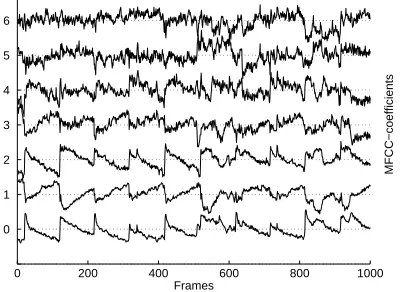
Figure 1 shows the first seven normalized MFCCs of a10second excerpt of the music piece Master of Revenge by the heavy metal group Body Count. As observed from the coefficients there is both temporal correlations as well as correlations among features dimensions.
0 200 400 600 800 1000 0
1 2 3 4 5 6
Frames
MFCC−coefficients
[image:2.595.320.520.287.433.2]MFCC coefficients of "Body Count − Masters Of Revenge" (10 seconds)
Figure 1: The first seven normalized MFCCs of a10second snippet of ”Body Count - Masters of Revenge”. The temporal correlation and correlations among feature dimensions are very clear from this piece of music.
2.2.1 Multivariate autoregressive model (MAR)
The multivariate autoregressive model handles both tem-poral and correlations among feature dimensions, which makes it a good candidate for feature integration. In [2] a simple autoregressive model was suggested where sim-ple refers to considering each feature dimension indepen-dently. The MAR model is popular in time-series mod-elling and prediction being both simple and well under-stood, see e.g. [7]. For a stationary time series of state vectorsxn∈ RDthe MAR model is defined by
xn=
K
X
p=1
Apxn−I(p)+µµµ+un, (2)
where the noise termun(error-term) is assumed to be zero mean Gaussian distributed, henceun ∼ N(un;0,C).
encode how much of the previous information given in
xn−I(1),xn−I(2), ..,xn−I(K)is present inxn. The above formulation is quite general as I refers to a general set. For a model order of K = 4, the set could be selected asI ={1,2,3,4}orI ={1,2,4,8} indicating thatxn
is predicted from these previous state vectors. In this pa-per we focus on the standard multivariate autoregressive model whereI ={1,2,3, . . . , K}. When estimating the parameters of the model there is several methods avail-able, see e.g. [7]. The authors have used the ARFIT pack-age, a regularized ordinary least squares approach, de-scribed in [8]. This package ensures the uniqueness of the estimated parameters of the model.
2.2.2 Multivariate Gaussian model (GM)
Neglecting the temporal correlations in the data, hence setting theApmatrices forp= 1, . . . , Kin equation (2) to zero leads to the much simpler model
xn =µµµ+un, (3)
whereµµµencode the mean value of the time series and
un ∼ N(u
n;0,C)is denoted the multivariate Gaussian
model. The previous mentioned mean-variance model is the mean valueµµµand the variance components given from the diagonal of the covariance matrixv= diag{C}.
If the full covariance matrix is used, only the upper (or lower) triangular coefficients are needed due to the sym-metry. The multivariate Gaussian model will be consid-ered as the ”base-line” against the MAR model in the ex-perimental section since it performs better than the typical
mean-variance model.
The two feature integration techniques described above can be used to derive features at the medium time
scale or used directly to derive features at the long time scale. The model order for the MAR model can be
se-lected from e.g. Schwarz’s Bayesian Criterion (SBC) [8], which is implemented in the ARFIT package or as in our experimental setup, where a separate validation set was used to determine the optimal model order across data ex-amples (music snippets).
2.3 Unique Solutions
Performing feature integration the model parameters are typically used as new feature vectors at the new time scale. If the model does not have a unique solution, two similar audio pieces could risk being classified as dissimilar. Con-sider using a mixture of Gaussian (MoG), given as
p(x|θθθ) =
K
X
k=1
p(k)p(x|k, θθθ),
wherep(k) (andPKk=1p(k) = 1) are the mixing pro-portions andp(x|k, θθθ) ∼ N(x;µµµk,Ck), as a feature
in-tegration model. Optimizing the model parameters from the likelihood function using e.g. the EM-algorithm does not necessarily provide a global maximum since the likeli-hood function has many local maximums. So using these model parameters (mixing proportions, means and covari-ances) directly in a classifier2would make no sense.
Re-2Stacked in a vector.
cent studies in kernels indicate that it is possible to inte-grate this type of complicated models in a kernel, see e.g. [9, 10]. The mixture of Gaussian model was considered as modelling music snippets in [6] and will be investigated as a feature integration model in section 4.
3
CLASSIFIERS
Earlier work in the field of music information retrieval (MIR) considered simple yet efficient classifiers such as K-nearest neighbors, however, lately more computation-ally demanding algorithms have been investigated. Only a few researchers within the field of MIR have consid-ered support vector machines (SVM), see e.g. [11, 12]. In the following subsections the support vector classifier (SVC) and the linear neural network classifier (LNN) will be briefly discussed.
3.1 Support Vector Classifier
The challenge of machine learning is to provide the learner with as broad a range of functions as possible while still ensuring that accurate learning can be achieved. Using high-dimensional feature spaces satisfies the first constraint of ensuring high flexibility, but appears to be at odds with the second since it is undermined by the curse of dimensionality. As a result we would expect that a good fit on the training data could still leave the generalization very poor. Support vector machines [13] manage to avoid this difficulty by optimizing a bound on the generalization error in terms of quantities that do not depend on the di-mension of the feature space [14], hence enabling good performance unaffected by the curse of dimensionality. In the present work, the C-library LIBSVM [15] was used. This library implements the one-against-one voting termi-nology to handle more than two classes.
3.1.1 Kernels
A typical applied kernel for the support vector classifier is the linear kernel, which is defined as
κ(x,x0
) =xTx0
, hence an inner product between the in-put vectors. Another well known kernel is the Gaussian kernel (or RBF-kernel) with width parameterσdefined as κ(x,x0
) = exp(− kx−x0
k2 /2σ2). Using this kernel the support vector classifier is basically finding discrimi-nating dimensions in an infinite feature space.
The linear and RBF kernel can be used in comparing vector data, however, when handling audio we are typi-cally forced to calculate the distance between two audio snippets of varying lengths, which for two pieces of audio is presented by the sequence of short time features: X=
[x1,x2, . . . ,xL]∈ RD×LandX0 = [x0
1,x 0 2, . . . ,x
0 L0]∈
RD×L0
. The two audio files are not required to be of same length, though in the present investigation they are (L =L0
). Two different kernels have been investigated, which calculate a similarity between sequences of data, the convolution kernel [16] and the product probability
kernel [9]. These kernels naturally incorporate feature
in-tegration.
Convolution Kernel - CK
structures such as strings, trees and graphs. In this work the convolution kernel measures the distance (correlation) between two audio pieces (between their feature vectors). The kernel is defined as
κ(X,X0 ) = 1
L2 L
X
v=1 L
X
v0=1
κI(xv,x 0
v0), (4)
whereκI(x,z)must be a valid kernel. It is interesting to note that if a linear kernel is used a fast calculation can be obtained.
Product Probability Kernel - PPK
The product probability kernel introduced in [9] measures the distance between probability models of the feature vectors. Other divergence based kernels have been sug-gested, see e.g. [10], for measuring a similar distance. In [6] the Kullback-Leibler similarity measure was applied to measure the distance between timbre models of mu-sic snippets modelled by a mixture of Gaussian, however, no closed form solution could be found using this diver-gence measure. With the product probability kernel, a closed form solution can be determined for e.g. a mixture of Gaussian, furthermore, the PPK fulfills the requirement for a kernel to be positive semi-definite. From [9] the PPK is given as
κ(θθθ, θθθ0 ) =
Z
p(x|θθθ)ρp(x|θθθ0
)ρdx, (5)
whereθθθ(θθθ0
) are the parameters from modellingX(X0 ), ρ > 0andp(x|θθθ)is the probabilistic model of the short time features of a music piece. ρ controls the weight-ing of low or high density areas of the probability dis-tribution. Selecting ρ = 1/2the Bhattacharyya affinity between distributions is found. A nice bi-product of se-lectingρ = 1/2 is a normalized kernel structure, since κ(θθθ, θθθ) =R p(x|θθθ)dx= 1. This kernel can directly
com-pute the distance between the models suggested in section 2.2, and thus incorporates feature integration. As men-tioned in section 2.3 the problem of uniqueness is allevi-ated for this kernel, since probabilistic models are com-pared instead of model parameters.
Closed form solutions of the kernel for the multivari-ate Gaussian and mixture of Gaussian can be found in [9]. Additionally, we have calculated a closed form solution of the MAR model, but the details have been omitted through lack of space3.
3.2 Linear Neural Network classifier (LNN)
The linear Neural Network hasc outputs and is trained using a squared loss function [17]. This classifier has pre-viously been applied with success in music genre classifi-cation, see e.g. [2, 4].
3.3 Fusion Techniques
The early information fusion (feature integration) was dis-cussed in section 2.2. Late information fusion is the
prob-3
Regarding computational complexity the methods ranked after numerical complexity are (top: least computational inten-sive): GM, MAR, MoG. The GM and MAR are closer related in complexity than the MAR and MoG.
lem of combining the results from the classifier. There ex-ist several ways of performing late information fusion, see [18]. In the present work, the majority voting rule was ap-plied due to the SVM classifier. In the majority vote rule, the votes received from the classifier are counted and the class with the largest amount of votes is selected, hereby performing consensus decision.
4
EXPERIMENTS
To evaluate the different feature integration techniques an 11 genre music setup was investigated. As discussed in the introduction, decisions can be made at different time scales. In the present work, the best achievable perfor-mance at30seconds will be pursued, using the above fea-ture integration techniques, voting technique and combi-nations of the two.
4.1 Data set
The data set consists of11music genres distributed evenly among the following categories: Alternative, Country,
Easy Listening, Electronica, Jazz, Latin, Pop&Dance, Rap&Hiphop, R&B and Soul, Reggae and Rock. The data
set consists of a training set of1098music snippets,100 from each genre except for latin, of each30seconds and a separate test set of220music snippets each of30seconds in length. The music snippets were MP3 encoded music with a bit-rate≥128kBdown-sampled with a factor two to22050Hz.
4.1.1 Human evaluation
To test the integrity of the data set a human evaluation was performed on the music snippets (at a30second time scale) of the test set. Each test person out of9was asked to classify each music snippet into one of the11genres on a forced choice basis. Each person evaluated33music snip-pets out of the220music pieces. No information except for the genre of the music pieces was given prior to the test. The average accuracy of the human evaluation across people and across genre was 51.8%as opposed to ran-dom guessing, which is∼ 9.1%. The lower/upper 95% confidence limits were 46.0%/57.7%(results shown in figure 2, upper figure). The human evaluation shows that the common genre definition is less consistent for this data set, however, it is still interesting to observe how an auto-matic genre system works in this setup.
4.1.2 Results & Discussion
In each genre90out of the100 music snippets from the training set were randomly selected10times to assess the variations in the data. In each of these runs the remaining music pieces (10in each genre, except latin) was used as a validation set for tuning parameters such asCin the sup-port vector classifier andσ in the RBF kernel. Optimal model order selection for the MAR models were deter-mined across music samples and evaluated on the valida-tion set. A model order ofK= 3at both2and30seconds was found optimal.
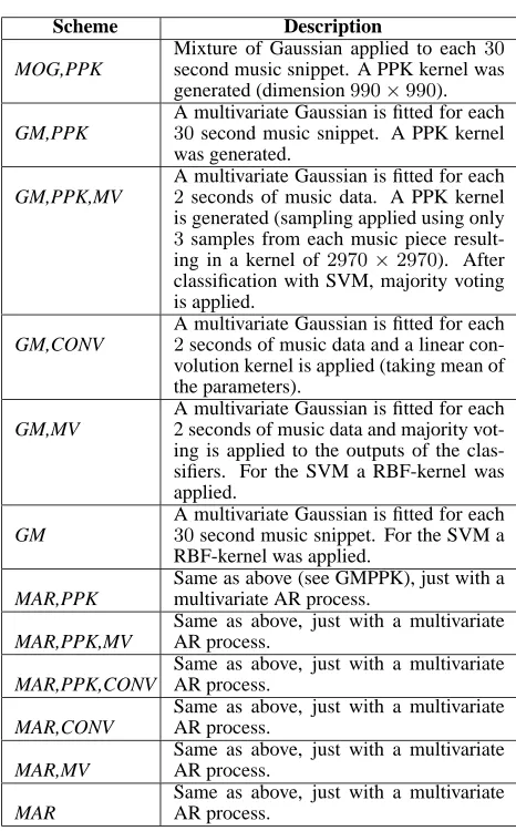
Table 1:Description of the different combinations investigated.
All investigations with the product probability kernel,ρ= 1/2
was used.
Scheme Description
MOG,PPK
Mixture of Gaussian applied to each30
second music snippet. A PPK kernel was
generated (dimension990×990).
GM,PPK
A multivariate Gaussian is fitted for each
30second music snippet. A PPK kernel
was generated.
GM,PPK,MV
A multivariate Gaussian is fitted for each
2seconds of music data. A PPK kernel
is generated (sampling applied using only
3samples from each music piece
result-ing in a kernel of2970×2970). After
classification with SVM, majority voting is applied.
GM,CONV
A multivariate Gaussian is fitted for each
2seconds of music data and a linear
con-volution kernel is applied (taking mean of the parameters).
GM,MV
A multivariate Gaussian is fitted for each 2 seconds of music data and majority vot-ing is applied to the outputs of the clas-sifiers. For the SVM a RBF-kernel was applied.
GM
A multivariate Gaussian is fitted for each
30second music snippet. For the SVM a
RBF-kernel was applied.
MAR,PPK
Same as above (see GMPPK), just with a multivariate AR process.
MAR,PPK,MV
Same as above, just with a multivariate AR process.
MAR,PPK,CONV
Same as above, just with a multivariate AR process.
MAR,CONV
Same as above, just with a multivariate AR process.
MAR,MV
Same as above, just with a multivariate AR process.
MAR
Same as above, just with a multivariate AR process.
MARMV method explained in table 1 varying the
frame-/hop size of the medium time scale4. No big performance fluctuation was observed in this investigation, however, a small favor of a frame-/hop size of 2/1second was ob-served. The various combinations investigated have been described in more detail in table 1. For the mixture of Gaussian model incorporated in a product probability ker-nel (MOG,PPK) the optimal model order for each music snippet of30seconds were selected by varying the model order between2−6mixtures, and selecting the optimal order from the Bayesian Information Criterion (BIC).
The average accuracy over the ten runs of the various combinations illustrated in table 1 have been plotted in fig-ure 2 (upper figfig-ure) with a95%binomial confidence ap-plied to the average values. From the accuracy plot there is a clear indication that the MAR model is performing better than the GM for both the SVM and LNN classifier. Performing a McNemar test, see e.g. [19], on the mixture of Gaussian model (MOGPPK) and the Gaussian model in a product probability kernel (GMPPK) the probability that
4
The investigated frame-/hop sizes were:{1s/0.5s, 1.5s/0.75s,
2s/1s, 2.5s/1.25s, 3s/1.5s, 3.5s/1.75s}.
0.25 0.3 0.35 0.4 0.45 0.5 0.55
MOGPPK GMPPK
GMPPKMV GMCONV
GMPPKCONV GMMV
GM MARPPK
MARCONV MARMV MAR
GMMV GM
MARMV
MAR
HUMAN
MARPPKMV MARPPKCONV
SVM LNN
Accuracy on Test−set
Accuracy
Models
−0.4 −0.2 0 0.2 0.4 0.6 0.8 1
MARMV(LNN)
MARPPK
Human
Accuracy of each genre
Accuracy
[image:5.595.56.289.104.479.2]Alternative Country Easy listening Electronica Jazz Latin Pop & Dance Rap & Hiphop R&b and Soul Reggae Rock
Figure 2:Upper: Average accuracy at30seconds shown with
a95%binomial confidence interval for all investigated
combi-nations. The larger confidence interval for humans is due to only nine persons evaluating a part of the test-data. Lower:
Aver-age accuracy with95%confidential interval of each genre at a
time scale of30seconds using the two best performing
combi-nations, MARMV and MARPPK. The average human accuracy
in each genre is also shown with a75%confidence interval.
the two models are equal is76%, hence the hypothesis that the models are equal cannot be rejected on a5% signifi-cance level. This observation, together with the good per-formance of the MAR model illustrate the importance of the temporal information in the short time features. Even with the various techniques applied in this setup we are still around ∼ 8%from the average human accuracy of
∼52%on this data set, but it is interesting to notice that reasonable performance is achieved with fairly simple fea-ture integration models and fusion techniques using only the first seven MFCCs. The two best performing mod-els are the MAR model in a product probability kernel (MARPPK) and the MAR model modelled at2seconds, after which majority voting is applied on the LNN outputs (MARMV), see figure 2 (upper). The McNemar test on these two models showed a43%significance level thus it can not be rejected that the two models are similar.
for the MARMV model a sequence of model parameters need to be saved for each music snippet. The computa-tional workload though, is a little larger for the MARPPK model when compared to the MARMV model.
Figure 2 (lower) shows the accuracy on each of the 11 genres of the two models MARMV and MARPPK. The MARPPK seem to be more robust in classifying all genres, whereas the MARMV is much better at specific genres such as Rap & Hiphop and Reggae. However, the MARMV does not capture any of the Rock pieces, but generally confuses them with Alternative (not shown here). Also illustrated in this figure is the human perfor-mance in the different classes. A confidence interval of 75%has been shown on the human performance, due to the few test persons involved in the test. The humans are much better at genres such as Rap & Hiphop and Reggae than, e.g. Alternative, which also corresponds to some of the behavior observed with the MARMV method.
5
CONCLUSION
The purpose of this work has partly been to illustrate the importance of modelling the temporal structure in the short time features, and secondly how models of short time features can be integrated into kernels, such that the support vector machine can be applied. In the music genre setup the best performance was achieved with the MAR model in a product probability kernel (MARPPK) used in combination with an SVM and with the MAR model used in combination with majority voting (MARMV) in a lin-ear neural network. The average accuracy of these two methods were∼ 43%compared to a human average ac-curacy of∼52%.
Even though the results presented in this article were a music genre setup, the general idea of feature integration and generating a kernel function, which efficiently evalu-ates the difference between audio-models can be general-ized and used in other fields of MIR.
ACKNOWLEDGEMENTS
The work was supported by the European Commission through the sixth framework IST Network of Excellence: Pattern Analysis, Statistical Modelling and Computational Learning (PASCAL), contract no. 506778.
REFERENCES
[1] G. Tzanetakis and P. Cook. Musical genre classifica-tion of audio signals. IEEE Transacclassifica-tions on Speech
and Audio Processing, 10(5), July 2002.
[2] A. Meng, P. Ahrendt, and J. Larsen. Improving mu-sic genre classification by short-time feature integra-tion. In Proc. of ICASSP, pages 1293–1296, 2005.
[3] D. Perrot and R. Gjerdigen. Scanning the dial: An exploration of factors in identification of musical style. In Proc. of Soc. Music Perception Cognition, 1999.
[4] P. Ahrendt, A. Meng, and J. Larsen. Decision time horizon for music genre classification using short-time features. In Proc. of EUSIPCO, pages 1293– 1296, 2004.
[5] M. F. McKinney and J. Breebaart. Features for audio and music classification. In Proc. of ISMIR, pages 151–158, 2003.
[6] J-J. Aucouturier and F. Pachet. Music similarity measures: What’s the use? In Proc. of ISMIR, 2002.
[7] Helmut L¨utkepohl. Introduction to Multiple Time
Se-ries Analysis. Springer-Verlag, 1993.
[8] A. Neumaier and T. Schneider. Estimation of param-eters and eigenmodes of multivariate autoregressive models. ACM Transactions on Mathematical
Soft-ware, 27(1):27–57, March 2001.
[9] T. Jebara, R. Kondor, and A. Howard. Probability product kernels. Journal of Machine Learning
Re-search, pages 819–844, July 2004.
[10] P. J. Moreno, P. P. Ho, and N. Vasconcelos. A kullback-leibler divergence based kernel for svm classification in multimedia applications. In
Ad-vances in Neural Information Processing Systems 16, Cambridge, MA, 2004. MIT Press.
[11] L. Lu, S. Z. Li, and Zhang H.-J. Content-based au-dio segmentation using support vector machines. In
ACM Multimedia Systems Journal, volume 8, pages
482–492, March 2003.
[12] S.-Z. Li and G. Guo. Content-based audio classifica-tion and retrieval using svm learning. In First IEEE
Pacific-Rim Conference on Multimedia, Invited Talk, Australia, 2000.
[13] N. Cristianini and J. Shawe-Taylor. An introduction
to Support Vector Machines. Cambridge University
Press, Cambridge, UK, 2000.
[14] J. Shawe-Taylor and N. Cristianini. On the generali-sation of soft margin algorithms. IEEE Transactions
on Information Theory, 48(10):2721–2735, 2002.
[15] C-C. Chang and C-J. Lin. Libsvm : A li-brary for support vector machines, 2001. (http://www.csie.ntu.edu.tw/ cjlin/libsvm).
[16] David Haussler. Convolution kernels on discrete structures. Technical report, University of Califor-nia at Santa Cruz, July 1999.
[17] C. M. Bishop. Neural Networks for Pattern
Recog-nition. Oxford University Press, 1995.
[18] J. Kittler, M. Hatef, Robert P.W. Duin, and J. Matas. On combining classifiers. IEEE Transactions on
Pat-tern Analysis and Machine Intelligence, 20(3):226–
239, 1998.