Compact local stencils employed with integrated RBFs for fourth-order differential problems

Compact Local Stencils Employed With Integrated RBFs

For Fourth-Order Differential Problems

T.-T. Hoang-Trieu1, N. Mai-Duy1and T. Tran-Cong1

Abstract: In this paper, new compact local stencils based on integrated radial basis functions (IRBFs) for solving fourth-order ordinary differential equations (ODEs) and partial differential equations (PDEs) are presented. The integration constants arising from the construction of IRBFs are exploited to incorporate into the local IRBF approximations values of the ODEs/PDEs at selected nodal points. The proposed stencils, which lead to sparse system matrices, are numerically val-idated through the solution of several analytic test problems. Numerical results indicate that their solutions converge very fast with grid refinement.

Keywords: Compact local approximations, high-order ODEs, high-order PDEs, integrated radial basis functions.

1 Introduction

Numerical techniques have been developed to solve ODEs and PDEs which are used to model continuum mechanics problems such as the motion of a fluid and the deformation of a solid body. Traditional discretisation methods include finite-difference methods (FDMs), finite-element methods (FEMs) and boundary-element methods (BEMs). Over the last 20 years, RBFs, which are known as a universal ap-proximator, have been applied for the solution of ODEs and PDEs. They were first developed as a global technique, in which the dependent variable is decomposed into a set of RBFs defined over the whole domain, and its derivatives are then calculated through differentiation (differentiated RBFs (DRBFs)) [Kansa (1990b)]. Later on, Mai-Duy and Tran-Cong (2001) proposed integrated RBF (IRBF) meth-ods, in which highest-order derivative(s) in the ODE/PDE are approximated by RBFs, and lower-order derivatives and the dependent variable itself are then ob-tained by integration. Numerical results showed that IRBFs yield better accuracy than DRBFs.

1_{Computational Engineering and Science Research Centre, Faculty of Engineering and Surveying,}

Global IRBF methods have some strengths and weaknesses. They can produce very accurate solutions using relatively low numbers of data nodes, and their implemen-tations are quite straightforward. However, they lead to fully populated system matrices. As a result, for a given spatial discretisation, larger requirements for computer’s storage are needed when compared with traditional methods. In addi-tion, the condition number of the global IRBF matrices grows very quickly as the number of nodes increases. To overcome these drawbacks, local and compact local IRBF schemes have been developed (e.g. [Mai-Duy and Tran-Cong (2009), Ngo-Cong, Mai-Duy, Karunasena, and Cong (2010), An-Vo, Mai-Duy, and Tran-Cong (2011), Mai-Duy and Tran-Tran-Cong (2011)]). The obtained system matrices are sparse and their solutions are thus more efficient. In Mai-Duy and Tran-Cong (2011), compact local IRBF stencils for solving Poisson equation on rectangular and non-rectangular domains were proposed; compact local forms are able to pro-duce much more accurate results than local forms.

This paper is concerned with the development of compact local IRBF stencils for the solution of fourth-order ODEs and PDEs. We will present a 5-node stencil for 1D problems and a 5×5-node stencil for 2D problems. The remainder of the pa-per is organised as follows. Section 2 is a brief review of IRBFs. The proposed compact local stencils based on IRBFs for 1D and 2D problems are presented in Section 3. Numerical examples are given in Section 4. Section 5 concludes the paper.

2 Brief review of integrated RBFs

Consider a fourth-order DE. In the IRBF methods, the highest-order derivatives (i.e. fourth-order ones under consideration here) of the field variableuare decomposed into a set of RBFs:

∂4u(η)

∂ η4 =

n

∑

wiI

(4)

i (η) (1)

where η denotes a component of the position vector x (e.g. η can be x for 1D

problems, andxoryfor 2D problems),{wi}ni=1is the set of RBF coefficients, and n

I_i(4)(x) on

∂3u(η)

∂ η3 =

n

∑

wiI_i(3)(η) +c1 (2)

∂2u(η)

∂ η2 =

n

∑

wiI

(2)

i (η) +ηc1+c2 (3)

∂u(η)

∂ η =

n

∑

wiI_i(1)(η) +η

2

2 c1+ηc2+c3 (4)

u(η) =

n

∑

wiI

(0)

i (η) +

η3

6 c1+

η2

2 c2+ηc3+c4 (5)

wherec₁,c₂,c₃andc₄are "constant of integration" with respect toη, which are to

be treated as the additional RBF coefficients. In (1) - (5), the superscript (.) is used to indicate the associated derivative order. In this study, the multiquadric (MQ) function is chosen as the basis function:

I_i(4)(x) = q

(x−ci)2_+a2

i for 1D problems (6)

I_i(4)(x) = q

(x−cix)2_{+ (y−ciy)}2_+a2

i for 2D problems (7)

whereci(for 1D problems) or(cix,ciy)T(for 2D problems) andaiare the MQ centre and width, respectively. The width of theith MQ can be determined according to the following relation:

ai=βdi (8)

whereβ is a factor (β>0) anddi is the distance from the ith centre to the nearest neighbour. It was observed in [Kansa (1990a)] that, as the RBF width increases, the numerical error of the RBF solution reduces and the condition number of the interpolant grows. At large values ofβ, one needs to pay special attention as the

solution becomes unstable. Values of β were reported to be 1 for global IRBF

methods and in a wide range of 2−200 for local and compact local IRBF methods. For the latter, one can vary the value ofβ and/or refine the spatial discretisation to

enhance the solution accuracy.

3 Proposed compact local IRBF stencils for fourth-order ODEs and PDEs

3.1 Compact local 5-node stencil for ODEs

Our sample of fourth-order ODEs is taken as

d4u dx4+

d2u

where xA ≤x≤xB and f(x) is some given function. The boundary conditions prescribed here are of Dirichlet type, i.e.uanddu/dxgiven atxAandxB.

We discretise the problem domain using a set ofndiscrete nodes. Consider a grid nodexi withi={3,4,· · ·,n−2}and its associated 5-node stencil[xi₁,xi₂,xi₃,xi₄,xi₅] (xi≡xi₃).

The conversion system, which represents the relation between the RBF space and the physical space, is established from the following equations

b u b e =

H(0)

K

| {z }

C b w b c (10)

where C is the conversion matrix, bu=H

(0)₍

b

w,bc) T

are equations representing nodal values ofuover the stencil,u_b= (u1,u2,u3,u4,u5)T,wb= (w1,w2,w3,w4,w5)

T_,

b

c= (c1,c2,c3,c4)T,H(0)is a 5×9 matrix that is obtained from collocating (5) at grid nodes of the stencil

H(0)₌

       

I₁(0)(xi₁), . . . , I₅(0)(xi₁), (xi₁)3/6, (x₁i)2/2, xi₁, 1

I₁(0)(x₂i), . . . , I₅(0)(xi₂), (x₂i)3_{/6, (x}i

2)2/2, x i 2, 1

I₁(0)(xi₃), . . . , I₅(0)(xi₃), (xi₃)3/6, (x₃i)2/2, xi₃, 1

I₁(0)(xi₄), . . . , I₅(0)(xi₄), (xi₄)3/6, (x₄i)2/2, xi₄, 1

I₁(0)(x₅i), . . . , I₅(0)(xi₅), (x₅i)3_{/6, (x}i

5)2/2, x i 5, 1

        b

e=K (w_b,_bc)T are equations representing extra information that can be the ODE (9) at selected nodes, anddu/dxatxAandxB. Solving (10) results in

b w b c =C−1

b u b e (11)

If the number of extra information values are less than or equal to 4, the obtained conversion matrix in (10) is not overdetermined owing to the presence of the inte-gration constants. In this case, the extra information is thus imposed in an exact manner.

xon the stencil are calculated in the physical space as

d4u(x)

x4 =

h

I₁(4)(x), . . . , I₅(4)(x), 0, 0, 0, 0 i

C−1

b u b e (12)

d3u(x)

dx3 = h

I₁(3)(x), . . . , I₅(3)(x), 1, 0, 0, 0 i

C−1

b u b e (13)

d2u(x)

dx2 = h

I₁(2)(x), . . . , I₅(2)(x), x, 1, 0, 0 i

C−1

b u b e (14)

du(x)

dx =

h

I₁(1)(x), . . . , I₅(1)(x), x2/2, x, 1, 0 i

C−1

b u b e (15)

u(x) =h I₁(0)(x), . . . , I₅(0)(x), x3/6, x2/2, x, 1 i

C−1

b u b e (16)

wherexi₁≤x≤xi₅.

In the following, two approaches for the construction of the final system of alge-braic equations, namely Implementation 1 and Implementation 2, are proposed. For each approach, we employe_b=K (w_b,c_b)T to represent values of (9) atxi₂and

xi₄, i.e.

f x₂i f x₄i

=

G1(x2i), . . . , G5(xi2), xi2, 1, 0, 0

G1(x₄i), . . . , G5(x₄i), xi₄, 1, 0, 0 b

w

b

c

wherei={3,4,· · ·,n−2}for Implementation 1, i={4,5,· · ·,n−3}for Imple-mentation 2 andGj(xik) =I

(4)

j x i k

+I(_j2) x_ki,k={2,4}.

Implementation 1:The final system is generated by the collocation of the ODE (9) at{x₃,x₄,· · ·,xn−2}using (12) and (14) withx=xi, and the imposition ofdu/dxat

xAandxB using (15) withx=x1andx=xn.

Implementation 2: The final system is generated by collocating the ODE (9) at {x4,x5,· · ·,xn−3} and{x2,x3,xn−2,xn−1}. For the former, the collocation process is similar to that of Implementation 1. For the latter, special treatments for the imposition of first derivative boundary conditions are required. Collocations of the ODE (9) at{x2,x3}and{xn−2,xn−1}are based on the stencils of nodesx3andxn−2,

respectively, with the following modified extra information vector

b

e= (du(xi₁)/dx,f(xi₄))T for the stencil ofx3 b

e= (f(xi₂),du(xi₅)/dx)T for the stencil ofxn−2

3.2 Compact local5×5-node stencil for PDEs

Consider a 2D fourth-order problem governed by the biharmonic equation

∂4u ∂x4+2

∂4u ∂x2y2+

∂4u

∂y4 = f(x,y) (17)

on a rectangular domain (xA≤x≤xB,yC≤y≤yD), and subject to Dirichlet bound-ary conditions (uand∂u/∂ngiven at the boundaries (nthe normal direction)).

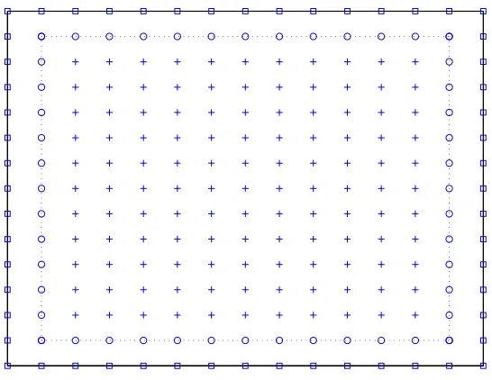
The problem domain is replaced by a Cartesian gridnx×ny, which is shown in Fig. 1.

Figure 1: A problem domain and a typical discretisation. Legends square, circle and plus are used to denote the boundary nodes, the interior nodes next the bound-ary and the remaining interior nodes, respectively.

1 2 3 4 5 6 7 8 9 10 11 12 13 14 15 16 17 18 19 20 21 22 23 24 25

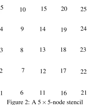
Figure 2: A 5×5-node stencil

The conversion system is constructed as

  b u b0 b e  =   

H(0)

x , O

H(0)

x , −Hy(0)

Kx, Ky



 

| {z }

C b wx b wy (18)

where the subscripts x andy denote the quantity associated with the integration process in thexandydirection, respectively, equationsHx(0)wbx=ubare employed to collocate the variable uover the stencil, equations Hx(0)wbx−H

(0)

y wby=b0 are employed to enforce nodal values ofuobtained from the integration with respect to

xandyto be identical, and equationsKxwbx+Kywby=ebare employed to represent extra information that can be values of the PDE (9) at selected nodes on the stencil and first-order derivative boundary conditions. In (18),C is the conversion matrix,

b

0 andOare a vector and a matrix of zeros, respectively,u_bandb0 are vectors of length 25; (wbx,wby)

T _{is the RBF coefficient vector of length 90, and O,H}(0)

x ,Hy(0),Kx andKy are matrices (the first three are of dimensions 25×45, while for the last two, their dimensions are dependent on the number of extra information values imposed and typically vary between 4×45 and 8×45). Solving (18) yields b wx b wy

We also propose two approaches, namely Implementation 1 and Implementation 2, to form the final set of algebraic equations.

Implementation 1: The final system is composed of two sets of equations. The first set is obtained by collocating the PDE and the second set is obtained by im-posing first derivative boundary conditions.

Implementation 2: First derivative boundary conditions are incorporated into the conversion system and the final system is formed by collocating the PDE only.

Some implementation notes:

1. In constructing the approximations for stencils, the cross derivative∂4u/∂x2∂y2

is computed through the following relation [Mai-Duy and Tanner (2005)], which requires the approximation of second-order pure derivatives only,

∂4u ∂2x∂2y=

1 2

∂2 ∂x2

∂2u ∂y2

+ ∂

2

∂y2

∂2u ∂x2

= 1 2

H(2)

x h

H(0)

x

i−1

H(2)

y wby

+Hy(2) h

H(0)

y

i−1

H(2)

x wbx

(20)

2. In constructing_be=Kxwbx+Kywby, we choose four nodes placed in the diamond in Fig. 2 (i.e(i−1,j),(i,j−1),(i,j+1)and(i+1,j)) to collocate the PDE (17).

KxandKycan thus be expressed in the form

Kx=H

(4)

x (x) +Hy(2)(x)

h

H(0)

y i−1

H(2)

x

Ky=Hy(4)(x) +Hx(2)(x)

h

H(0)

x i−1

H(2)

y

wherexrepresents the coordinates of the four points{8,12,14,18}.

3. The collocations of (17) at four interior "corner" nodes (i.e. (2,2),(2,ny−1), (nx−1,2)and(nx−1,ny−1)) are based on the stencils of four nodes(3,3),(3,ny− 2),(nx−2,3)and(nx−2,ny−2)with the modified extra information vectors. For example, in the case of(2,2), we modifye_b=Kxwbx+Kywbyas

              

∂u(x2) ∂x ∂u(x3)

∂x ∂u(x6)

∂y ∂u(x11)

∂y f(x14)

f(x18)                =          

H(1)

x (x2), O

H(1)

x (x3), O

O, Hy(1)(x6)

O, Hy(1)(x11)

G_[x](x14), G[y](x14)

wherex= (x,y)T_,

G_[x](xk) =Hx(4)(xk) +Hy(2)(xk) h

H(0)

y i−1

H(2)

x , and

G_[y](xk) =Hy(4)(xk) +H

(2)

x (xk) h

H(0)

x i−1

H(2)

y , k={14,18}

Both Implementation 1 and Implementation 2 lead to a final system matrix of di-mensions(nx−2)(ny−2)×(nx−2)(ny−2).

4 Numerical examples

We measure the accuracy of an approximation scheme in the form

Ne(u) = r _n

∑

i=1

(ui−uei)2 r _n

∑

i=1 (ue_i)2

(22)

wheren is the number of collocation nodes, andui anduei are the computed and exact solutions, respectively. The convergence rateα of the solution is estimated

viaNe(u)'O(hα_{), in whichhis the grid size.}

Apart from the grid-refinement study, we will also investigate the effects of the MQ width on the solution accuracy.

4.1 One-dimensional problem

Consider the following fourth-order ODE

d4u dx4+

d2u dx2 =16π

4_sin(2

πx)−4π2sin(2πx), 0≤x≤2 (23)

Boundary conditions are defined asu=0 and du

dx =2π atx=0 andx=2.

The exact solution to this problem can be verified to beue(x) =sin(2πx).

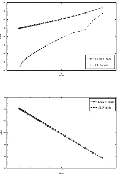
Various grids, (7, 9,..., 71), are employed. Fig. 3 shows the accuracies of the solu-tion and condisolu-tion numbers of the system matrix against the grid sizeh. Results by local 5-node stencil are also included for comparison purposes. It can be seen that compact local IRBF stencils have similar values of the matrix condition number but yield much more accurate results than local IRBF stencils. The solution converges apparently asO(h5.31)for the former andO(h2.18)for the latter.

10−1 10−7

10−6 10−5 10−4 10−3 10−2 10−1 100 101

xlabel

ylabel

Local 5−node

CL 5−node

10−1 101

102 103 104 105 106 107

xlabel

ylabel

Local 5−node CL 5−node

Figure 3: ODE, β =19: solution accuracy and matrix condition number against

the grid size

However, Implementation 2 yields better condition numbers than Implementation 1, probably owing to the fact that the final system matrix of the former is composed of equations derived from the PDE only.

As mentioned earlier, the value ofβ would have a strong influence on the solution

accuracy. Since the exact solution to this problem is available, it is straightforward to obtain the optimal value ofβ (i.e. at whichNe(u)is minimum). Table 1 shows results obtained by a fixed value and the optimal value ofβfor three different grids.

It can be seen that using the optimal value ofβ significantly enhances the solution

accuracy.

Several remarks can be made as follows.

10−1 10−7

10−6 10−5 10−4 10−3 10−2 10−1 100

xlabel

ylabel

Local 5−node

CL 5−node

10−1 101

102 103 104 105 106 107 108 109

xlabel

ylabel

Local 5−node

CL 5−node

Figure 4: ODE, β =19: solution accuracy and matrix condition number against

the grid size

Table 1: ODE: Solution accuracy using a fixed value and the optimal value ofβ for

three different grids.

h 1₂₀ 1₅₀ 1₇₀

β =19

Ne(u) 7.08E-4 6.09E-6 1.89E-7

Optimalβ

4.3 12.9 19

(ii) The solution accuracy can be effectively controlled by means of the RBF width. (iii) Implementation 2 performs better than Implementation 1.

4.2 Two-dimensional problem

Consider the biharmonic problem with the source function f(x,y) =16(1+π4−

2π2)[sin(2πx)sinh(2y) +16 cosh(4x)cos(4πy)], the domain−1/2≤x,y≤1/2 and boundary conditions of Dirichlet type.

The exact solution isue(x,y) =sin(2πx)sinh(2y) +cosh(4x)cos(4πy).

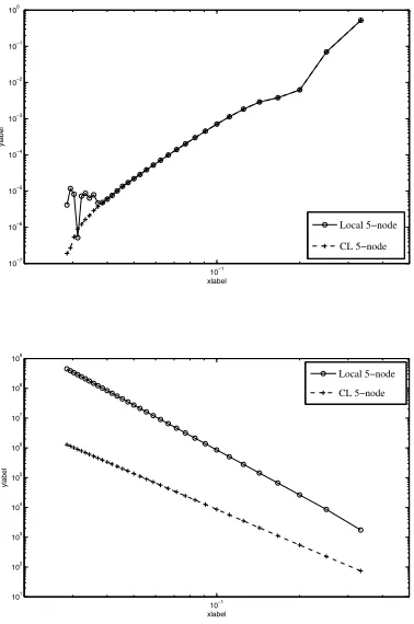
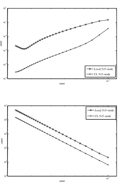
Calculations are carried out with various grids of densities (11×11,13×13, ...,71× 71) for both local and compact local IRBF stencils. Fig. 5 displays the solution ac-curacy and matrix condition number usingβ = 3 for various values of grid sizeh.

The obtained results indicate that compact local 5×5-node IRBF stencils outper-form local 5×5-node IRBF stencils regarding accuracy and stability (i.e. lower condition numbers). The local and compact local solutions converge asO(h2.14) andO(h4.14), respectively, while their matrix condition numbers grow asO(h−4.0) andO(h−3.88), respectively. It is also shown that the compact version works better than the standard version at fine grids.

Fig. 6 compares the solution accuracy and the matrix condition number between the two implementations of the proposed IRBF method, and Table 2 shows a com-parison of the solution accuracy between the case of a fixedβ value and the case of

the optimal value ofβ. Remarks here are similar to those for 1D problems.

Table 2: PDE: Solution accuracy using a fixed value and the optimal value ofβ for

three different grids.

h 1₁₀ 1₂₀ 1₃₀

β =3

Ne(u) 3.64E-2 1.54E-3 4.86E-4

Optimalβ

1.32 6.86 8.52

Ne(u) 3.38E-2 9.21E-4 4.65E-4

5 CONCLUDING REMARKS

10−1 10−5

10−4 10−3 10−2 10−1 100

xlabel

ylabel

Local 5×5−node

CL 5×5−node

10−1

102

103

104

105

106

107

xlabel

ylabel

Local 5×5−node

CL 5×5−node

Figure 5: PDE,β =3: accuracy and matrix condition number against the grid size

in terms of not only nodal values of the field variable but also nodal values of the ODE/PDE. The latter is incorporated through the conversion system with the help of the integration constants. The proposed stencils are successfully verified; numerical results show that high convergence rates are obtained. However, special treatments are required for the interior nodes next to the boundary. This problem is currently investigated and the outcome will be reported in our future work.

10−1

10−5

10−4

10−3

10−2

10−1

xlabel

ylabel

Local 5×5−node CL 5×5−node

10−1

102

103

104

105

106

107

108

109

1010

xlabel

ylabel

Local 5×5−node CL 5×5−node

Figure 6: PDE,β=3: Accuracy and matrix condition number against the grid size

References

An-Vo, D.-A.; Mai-Duy, N.; Tran-Cong, T.(2011): A C2-continuous Control-Volume technique based on Cartesian grids and two-node integrated-RBF elements for second-order elliptic problems. Computer Modeling in Engineering & Sci-ences, vol. 72, pp. 299–334.

Kansa, E.(1990b): Multiquadrics - A scattered data approximation scheme with applications to computational fluid-dynamics - II Solutions to parabolic, hyperbolic and elliptic partial differential equations. Computers & Mathematics with Appli-cations, vol. 19 (8-9), pp. 147–161.

(8-9), pp. 127–145.

Mai-Duy, N.; Tanner, R. (2005): Computing non-Newtonian fluid flow with radial basis function networks. International Journal for Numerical Methods in Fluids, vol. 48(12), pp. 1309–1336.

Mai-Duy, N.; Tran-Cong, T.(2001): Numerical solution of differential equations using multiquadric radial basis function networks. Neural Networks, vol. 14, pp. 185–199.

Mai-Duy, N.; Tran-Cong, T. (2009): A Cartesian-grid discretisation scheme based on local integrated RBFNs for two-dimensional elliptic problems. Computer Modeling in Engineering and Sciences, vol. 51(3), pp. 213–238.

Mai-Duy, N.; Tran-Cong, T. (2011): Compact local integrated-RBF approxi-mations for second-order elliptic differential problems. Journal of Computational Physics, vol. 230, pp. 4772–4794.