Peristaltic motion

PERISTALTIC MOTION

by

Trevor Parkes) B.Sc. (Manchester) December)

1967

1. INTRODUCTION AND SUMMARY 2. HISTORICAL SURVEY

3

.

STATEMENT OF THE PROBLEM 4. SOLUTION OF T:HE PROBLEM

4.1

Peristalsis with constant pressure gradient and G small

4.

2

The general case of peristalsis with sinusoidal pressure

gradient and with G large

4.

3

Average flux in particular cases

5.

NUMERICAL CALCULATIONS OF FLUX, STREAMLINES AND VELOCITY DISTRIBUTION

5.1 Peristalsis with zero pressure gradient and G small

5.

2

Fixed boundary with prescribed constant pressure gradient

5.

3

Peristalsis with zero pressure gradient and G large

5

.

4

Fixed boundary with sinusoidal pressure gradient

5

.

5

Peristalsis with sinusoidal pressure gradient

6.

DIRECT CALCULATION OF THE COEFFICIENTS an, bn

6.1

Evaluation of the coefficients cnr, etc.

6.

2

Application of the method

7

.

OTHER BOUNDARY CONDITIONS

8.

CONCLUSION

APPENDIX A APPENDIX B

Page l

4

8 12

45

61

62

64

---~11

Page

REFERENCES

74

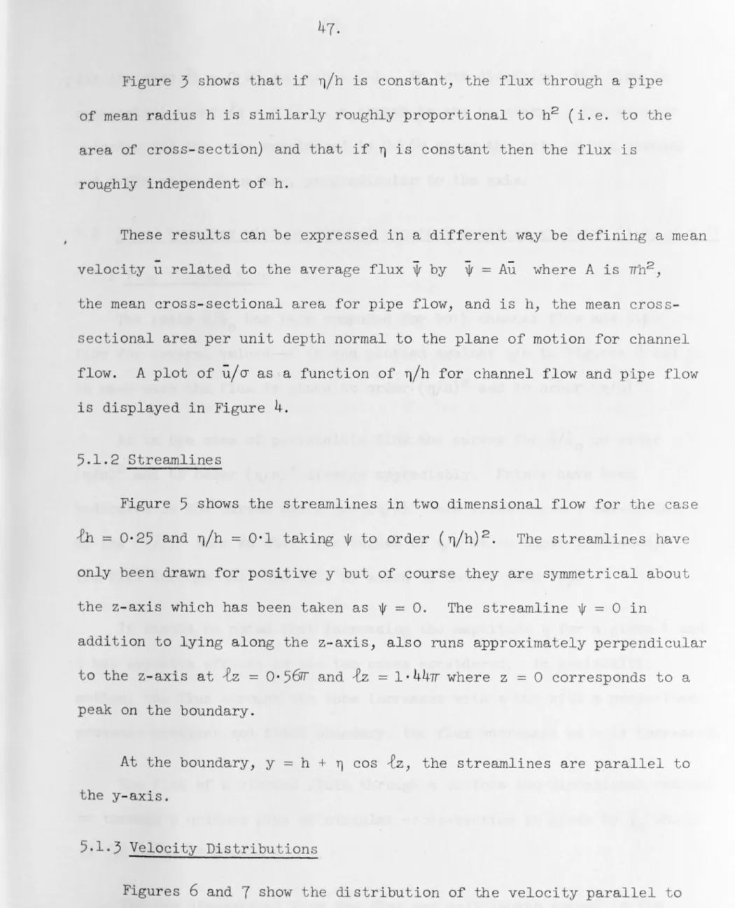
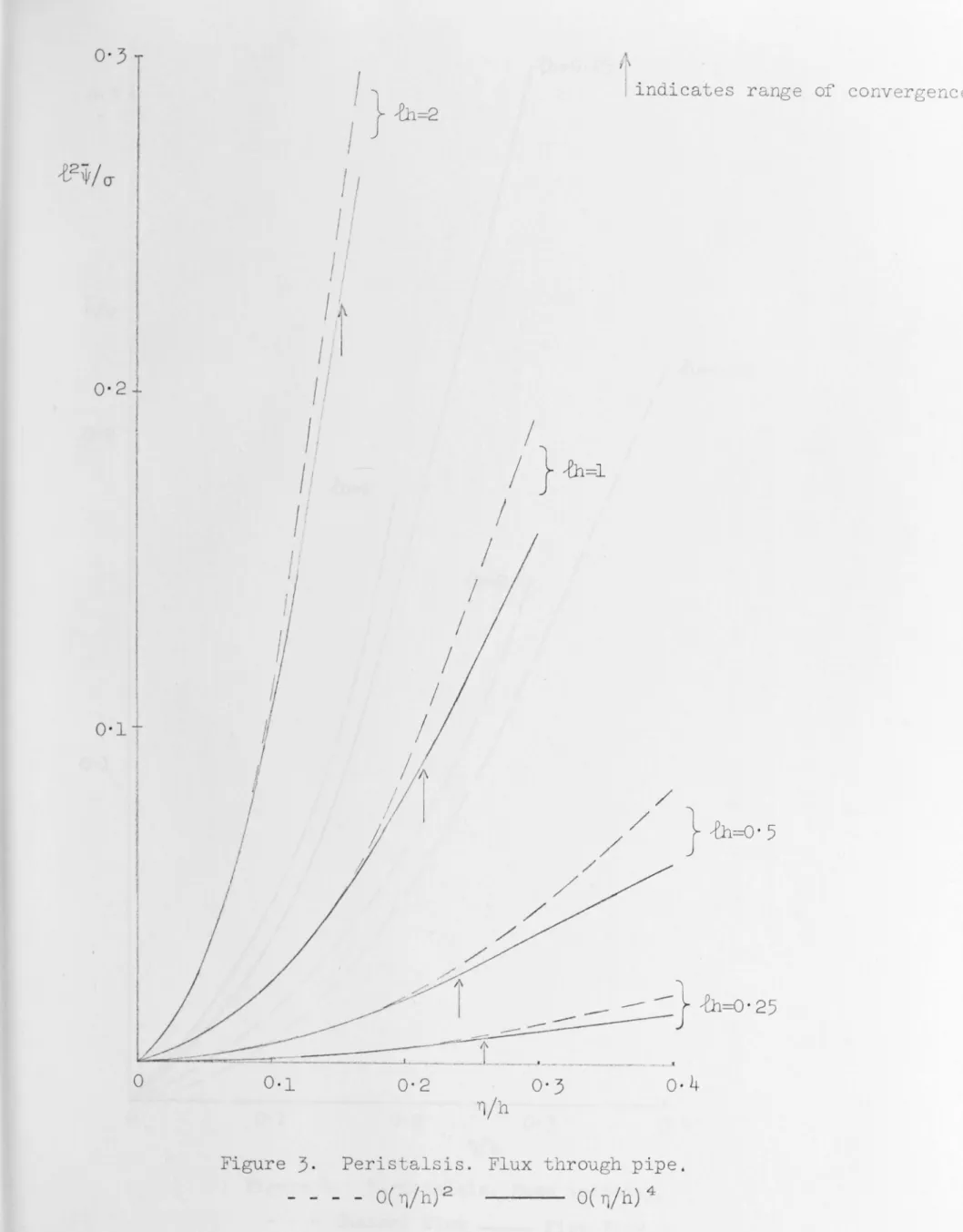
Figure 2. Peristalsis. Flux through channel. er small. Figure

3

.

Peristalsis. Flux through pipe. er small.

Figure

4

.

Peristalsis. Average velocity through pipe and channel.

Figure

5

.

Peristalsis. Streamlines in channel flow.

Figure

6

.

Peristalsis. Velocity distribution along axis in channel flow.

Figure

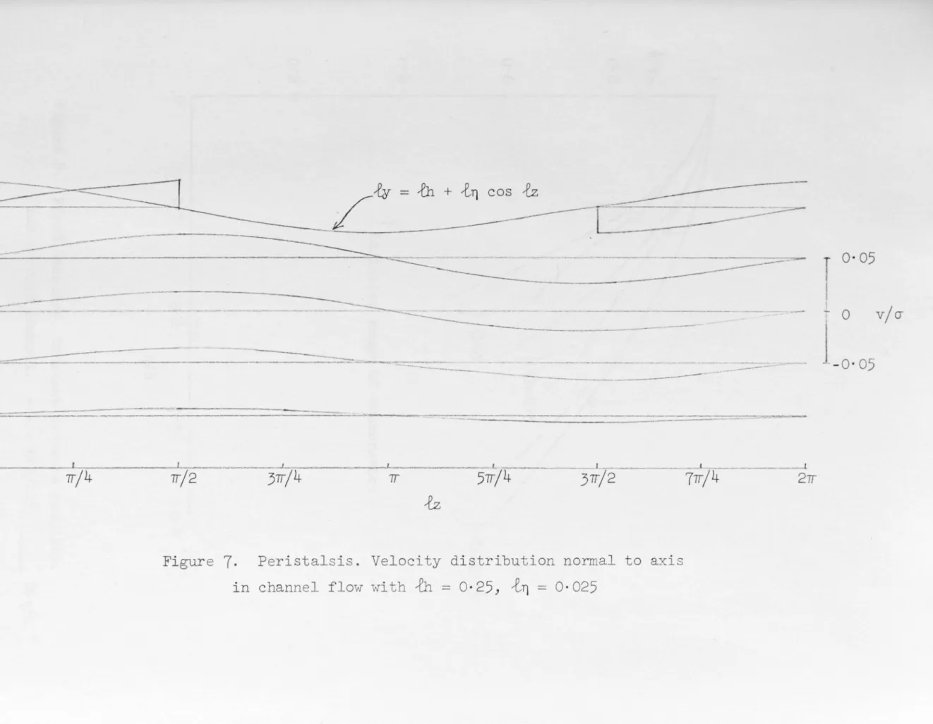
7.

Peristalsis. Velocity distribution normal to axis in chanriel flow.

Figure

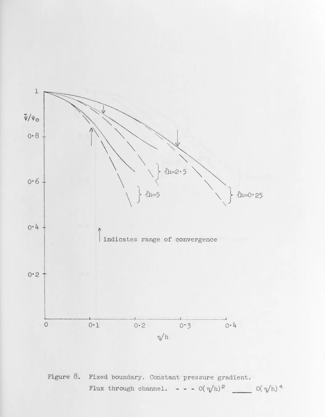
8

.

Fixed boundary. Constant pressure gradient. Flux through channel.

Figure

9

.

Fixed boundary. Constant pressure gradient . Flux through pipe.

Figure 10. Fixed boundary. Sinusoidal pressure gradient. Flux through channel.

Figure 11. Fixed boundary. Sinusoidal pressure gradient. Flux through pipe.

Table 2. Table

3

.

Table

4

.

Table 5.

Peristalsis. Flux through channel. Direct method.

Peristalsis. Comparison of flux through channel using both methods.

Fixed walls. Flux through channel. Direct method. Fixed walls. Comparison of flux through channel using both methods.

I should like to thank my supervisor Dr. J .C. Burns who suggested

the topic and who has been a constant source of encouragement. I should

also like t o thank my colleagues of the Mathemati cs Department, Royal

Military College, Duntroon, with whom I have had useful discussions, and

Mrs. G. Whyatt who so ably typed this thesis.

The material reported in this thesis is the author ' s work except where

references t o other sources are explicitly stated.

1. Introduction and Summary

The study of the flow of an incompressible viscous liquid is greatly simplified if discussion is limited to Stokes flow in which the Reynolds

r u m - ~

number is small enough for the~inertia forces to be neglected in

comparison with the viscous forces so that the equations of motion

become linear. The Stokes flow approximation is a suitable model to take for peristaltic motion since the velocities met in practice are small and conditions at infinity are not considered.

In this thesis, two dimensional flow through a symmetrical channel

and axially symmetric flow through a pipe of circular cross-section are

considered. In each case the boundary varies sinusoidally.

Two causes of motion are studied. Firstly, it will be assumed

that there is a prescribed pressure gradient along the pipe or channel

and secondly that a progressive wave passes along the walls. If the prescribed pressure gradient is constant, and if the progressive wave

velocity is small enough, this peristaltic motion is governed by the

usual equations for steady Stokes flow. Thus --the two extreme cases, of motion caused solely by the variation in cross-section and of motion

under a constant pressure gradient when the walls are fixed can be

treated together. Moreover, the two cases of pipe flow and channel flow can be treated together by taking advantage of the notation of generalized axi-symmetric potential theory to develop the theory in a

form which is applicable to each case, leaving only the detailed

calcu-lations to be carried out separately. This simpler case is treated first .

If the prescribed pressure gradient varies sinusoidally with time then

the motion is governed by the unsteady Stokes flow equations. In this

case there is nothing to be gained by imposing the condition that the

progressive wave velocity should be small and so the general case of

peristalsis with sinusoidal pressure gradient has been solved.

It will be convenient, where it is not necessary to distinguish

between channel flow and pipe flow, to use "tube" to denote either the

symmetric channel or the axi-symmetric pipe and "radius of the tube" to

denote half the breadth of the channel or the radius of the pipe.

The problem is solved by expanding the stream function, which

detennines the flow, as a Fourier series involving two infinite sets of

unknown coefficients, real in the simple case but complex in general.

The boundary conditions on the wall of the tube give a set of linear

equations which can be solved for these coefficients . Following closely

the method used by Taylor

(1951)

in a similar problem, a perturbation

solution is found in which these coefficients are derived as power

series _{in ri/h,} the ratio of the amplitude of the variation of the tube

radius to the mean tube radius. The solution is used to derive an

expression for _{the average flux through the tube in the general case.}

This average flux is calculated numerically in some particular cases,

are the streamlines and the velocity distributions along and normal to

the axis of the tube.

An alternative method of direct calculation of the unknown

coefficients has been devised and tested in particular cases. This

3.

method works well for small {~, where it would be expected to do so, and agrees with the perturbation method. It should work better than the

2. Historical Survey

Peristaltic motion of a viscous fluid through pipes and channels

does not appear to have been discussed previously mathematically although the particular case of flow under a prescribed pressure gradient through a fixed tube whose walls vary sinusoidally has been treated by several authors. Langlois

(1

96

4)

discussed f ow along channels of varying breadth and obtained approximate solutions in several different cases. Gheorgita (1959) found solutions to the first order in~ f or symmetrical channels in which the breadth varies along the length according to a cosine law and also gave first order solutions in cases in which the distance of each wall from the centre plane varies periodically along the length with the same frequency but the channel is not symmetrical. Belinfante(1962) considered flow of a viscous fluid along pipes and channels in which the radius or breadth varies along the length according to a cosine law. He also obtained solutions for the Stokes flow approximation correct to the first order in ~/h_. He used these solutions as a basis for solutions of the Navier-Stokes equations in powers of the Reynolds number of the flow.

He remarks that he has also obtained solutions of the Stokes flow.problem to the second order in ~/h for both pipe and channel flow. Burns (1965) used the methods of this thesis to obtain results for both pipes and

channels with fixed walls, which is a special case of the general

problem.of peristaltic flow with sinusoidal pressure gradient considered here. It is also, of course, a special case of peristaltic flow with

5.

The analysis of peristaltic motion may have several import ant

practical applications. Peristalsis occurs naturally in several parts

of the body. According to Wright

(1961)

"Bayliss and Starling defined

true peristalsis as a coordinated reaction in which a wave of contraction

preceded by a wave of relaxation passes down a hollow viscus; the contents

of the viscus as they are propelled along would thus always enter a

segment which had actively relaxed and enlarged to receive them. This

type of movement was thought to be responsible for transferring the

contents of the alimentary canal from the oesophagus through the stomach,

small and large intestine and finally to the anus." Peristaltic waves

also occur in the ureter.

The flow of corrosive fluids along pipes is often brought about by

the use of peristaltic pumps which are designed so that the fluid does

not come into contact with the pump itself. Latham and Shapiro

(19

66)

have done some work on peristaltic pumping but this paper is not yet

available.

The flow of blood in arteries, while not being caused by peristaltic

-motion of the artery walls, has similarities, particularly if it is

assumed that the artery walls are sufficiently flexible so that they

oscillate in sympathy with the pressure gradient. For this reason it

seemed logical in this thesis to consider the general case of peristalsis

with sinusoidal pressure gradient. However it must be realised that the

Reynolds number associated with blood flow in arteries is not small, and

The particular case of flow through a fixed pipe of constant cross

section under a prescribed sinusoidal pressure gradient has also been

treated by several authors but the more general case of a pipe whose

walls vary sinusoidally does not appear to have been considered.

Womersley was very prolific on this subject both theoretically and

experimentally. Amongst other things, he (1955) considered the

oscil-latory motion of a viscous liquid in a rigid tube under a simple harmonic

pressure gradient and also similar motion in a thin walled elastic tube

with particular reference to the flow of blood in arteries. In the latter

case he showed that the longitudinal oscillation of the walls of the tube,

caused by viscous drag on its inner surface, is important in determining

the rate of flow, which may be 10%,greater than that in a rigid tube

under the same pressure gradient. Olsen and Shapiro (1967) considered

large amplitude, unsteady flow in liquid filled elastic tubes but only

where the wave-length is long compared with the diameter

(-Di<

0·06) so

that a one dimensional model can be used. Lance (1956) considered the

flow through a pipe or channel of constant cross section due to a pressure

gradient and a series of pulses acting in the opposite direction. He

showed that it is possible for the flow to be arrested when the pipe is

subjected to one or more pulses of sufficient strength. (This problem

was suggested by reports that the engines of a certain jet aircraft fail

when the guns are fired. The failure could be due to fuel starvation.)

Sanyal (1956) studied the flow in a circular tube under pressure gradients

which rise or fall exponentially with time. She found that for small

7

.

is parabolic in both cases but for large diameter tubes the two motions

are quite different. In the first case the flow has the boundary layer

character while this characteristic is completely absent in the second

case and the velocity depends on the wall distance.

3.

Statement of the Problem

It is convenient to use "tube" to denote either the symmetrical

channel or the axi-symmetric pipe and "radius of tube" to denote half

the breadth of the channel or the radius of the pipe.

The wall of the tube is defined by the equation

y h + 'fl COS {_( X - ot)

(1)

so that a progressive wave of amplitude Tl, velocity rr and wave-length

A=

2v/t

passes along the tube in the positive x-direction. It will

frequently be convenient to write z

=

x - ot. If rr

=

o,

the wall of

the tube is a fixed cosine wave. The x-y plane is a meridian plane of

the tube, the axis OX being along the axis of symmetry and the axis OY

normal to OX. Let the velocity components in the x,y directions be u,v

respectively (see Figure 1).

9

.

The equations of motion governing the flow of an incompressible

fluid through the tube are the continuity equation and the Navier-Stokes

equation. These, in the absence of body forces, are

0 J ( 2)

av

1

~ + V(!v2) - V X ill

=

-

-

'vP - VV X Q.) ,

at

2- - - ( 3)

where y is the velocity, vis the kinematic viscosity, pis the pressure,

pis the density and~= V x

y

is the vorticity (Rosenhead

1963).

If squares of velocities can be neglected then equation (3) reduces

to

av

-at

1

- Vp - VV X ill.

p

It is possible to treat the two dimensional flow and the

axi-symmetric flow together by using the notation of generalized axially

symmetric potential theory (Weinstein

1953).

Let* be a stream function such that

u

=

y -k -

a

_ay

*

and V -k

81lr -y ..:::..:i:.

..

ax

where k

=

0 or l according as the flow is two dimensional or

axi-symmetric. Then equation (2) is satisfied.

and

If ill -

l~I

then the equations satisfied by* and w are

k - -y (1)

L ( k ) l

a (

ykw\ ,

-k Y w

=

v

at

~

( 4)

( 5)

( 6)

where

32

+

-ay2

k 8

y 8y •

Also equation

(4)

produces the following pressure relations:

au - p

-at

-k 8 k

µy ay ( Y ill) '

av

-k a k

- P at + µy

ax (

Y ill) '

whereµ - pV is the viscosi ty.

( 8)

( 9)

The following conditions must be satisfied. On the axis of symmetry \jr

=

0 and ill+ 0 as y + O. On the outer boundary of the flow, the fluid

must have the same velocity as the wall of the tube. It will be assumed in the first instance that the particles of the tube wall move in

straight lines perpendicular to the axis of the tube so that the boundary

condition i s

-k

21

-y 8z

-k 8\jr

Y

=

u - 0 , 8y

V ay

at {cn1 sin

{z

on y

=

h +~cos

{z

.

This condition requires that the wall of the tube be extensible. A modified boundary condition will be considered later in Section

7.

(10)

The problem is to solve equations

(6)

and

(7)

for \jr and ill subject to

these conditions on the axis of symmetry and the wall of the tube.

It is necessary to prescribe the pressure gradient which produces

11.

drop over a wave-length has the value P cos ft. In particular, P 0

corresponds to peristalsis with zero pressure gradient and f 0

4

.

Solution of the problem

It is convenient to deal with a particular case first and then

consider the general case. It is assumed that the flow has existed long

enough for all transient terms to have decayed so that only the steady

state solution is considered.

4

.1

Peristalsis with constant pressure gradient and~ small

i . e. f = 0 and

~/tv

= o (1)

This is the case of peristalsis with constant pressure gradient

av

where the progressive wave velocity is small enough for the term

at

in

equation

(4)

to be neglected (Rosenhead

1963).

An account of this has

already been published (Burns and Parkes

1967).

and

The equations to be solved are now

k -y (1)

0

with the conditions*= 0 on y = O and w ~ 0 on y = 0.

The boundary conditions (10) are unchanged. The pressure

relations

(8)

and

(9)

become

-k

a

k -µy ay ( Y w)

and ~

ay

-k

a (

k

µy

ax

Y w)

( 6)

( 7A)

( 8A)

( 9A)

Since the boundary varies periodically with z and is symmetrical

about z = O, it follows that both* and ware even periodic functions of

13.

00

1jr(z,y) -

l

1jr ( y) cos n~ ,

(

11

)

n n=O

00

ul..z,y) -

l

Cl.h ( y) cos n{z .

( 12)

n=O

If

(11)

and

(12)

are substituted in equations

(6)

and

(7A)

and the

coefficients of terms in cos n~ compared, then for n ~

o,

1jr (y) and

n

llb(y) satisfy the equations

k

-y CD _n '

-

o.

Tnese equations have to be solved under the conditions that

*n + 0 and CDn +Oas y +

o

.

The solutions of (14) satisfying these conditions are

and for n ~ 1

k y Clb

k

y CD

n

_ -A yk+l

0

k+l

- -A y 2

n (n~)

where A, _o A are _n arbitrary constants and Iv(x) is a modified Bessel

function of the first kind of order v.

(13)

(14)

( 15)

When CD _n in equation

(13)

is replaced by the expressions given in

integrals can be found (Burns

(19

6

6))

and the complementary functions

are of course the general solution of equation (14). The functions

o/ (y) which satisfy these equations and the condition o/ ~ 0 as y ~ 0

n n

are found without difficulty and when these are substituted in (11) the resulting expression for o/(zJy) is

o/(zJy) _2(k Ao

₃₎

y k+3 + Boy k+l

+

00 k+l

l

-

2 [2~:P, yik-1 ( n-fy) Bnik+l(n-fy)

J

cos n{z.

+ y +

n=l 2 2

( 16)

The arbitrary constants AnJ Bn for n ~ 0 must be determined from the

condition (lO)J that the fluid on the boundary has the same velocity as the wall of the tubeJ together with the condition that the pressure drop

per wave-length is P.

J.t

~

~

AR..J>rl\.

~

tL.t,

~

L

o

..;;

,,

e<

,u

Yn/,1;_

~

~

~

J!:

J

t

-

rd

~ryt~boP

~~

~ a n be s~n from equation (9A) that~ is an odd periodic function

of z. Hence~~= OJ i .e. pis constant) on the sections z = OJ AJ 2A ...

of the tube. It can also be seen from equation (BA) that!~ = ~ will be an even periodic function of z and so the £ressure difference between successive points of maximum cross section is always the same. In this

case it is assumed to be P.

Since the pressure is constant over the sections z = OJ A it

follows that the pressure drop between these sections can be obtained by integrating~ along the line y = O.

15.

Equation (8A) gives

~

oz

-µy - k -ay

a

(y k ru)

and this, with

(12)

and

(15),

leads to

00

µ(k + 1) A

0 +

I

fn cos n-tz , n l

where the coefficients fn are constants. Integration of

(17)

from

z = 0 to z = A gives

p~

- 2µ7T( k + 1)

( 1 7)

(18)

Thus the constant A₀ is known in terms of the prescribed pressure

gradient. The remaining boundary condition leads to equations sufficient

to determine the constants B₀, ~ , Bn (n ~

1)

in terms of A

0 and~.

At this point it becomes convenient to give separate (although

closely similar) discussions of the two cases of channel flow and pipe

flow.

For channel flow, k

=

0 and the stream function becomes

'lr(z,y)

b

Ao y3 + Boy

cosh n,fy + Bn sinh n,fy} cos n-tz.

( 19)

The replacement of the Bessel _{functions I1(niy) and I 1(n,cy-)} by

'2 - '2

expressions involving cash niy and sinh n,cy- leads to a considerable

simplification in the detailed analysis which follows.

For pipe flow, k

= 1 an

d the stream function becomes

\jr(z,y) Ao y4 + _Boy2

b

00

+

I

y {2~'.t ylo( n,fy) + BnI1 (n,fy)} cos n-i'z. n l

It is convenient to introduce new coefficients as follows :

For channel flow, let

and, for n ~ 1,

and for pipe

and, for n ~

a n flow, ao 1, an let !A

2 0 '

!A 2 0 )

An 2nt )

b

0

b n

) b

n

2B₀ ,

B . n

The stream function for channel flow then becomes

\jr(z,y)

00

( 20)

( 21)

( 22)

+

I

{any cosh n,fy + bn sinh n,fy} cos n-i'z ( 23)

n l

ch/r

=

₀

ay

and

oz

o\jr

-1

7.

sin .{z on y

=

h + T) cos {z

which are obtained from (10) by putting k - O.

The stream function for pipe flow becomes

- 1 a y4 + ! b

y2

4 0 2 0

00

+

I

Y {any I_{0 (} n,fy) + bnI_{1 (} n,fy)} cos n--tz

n l

(

24)

( 25)

where b₀, an, bn (n ~ 1) are to be found in terms of a

0 and~ from the

conditions

1 o\jr

Y

ay

- 0 and 1 y 8\jr

oz

_ _ {o-T) sin {.z

which are obtained from (10) by putting k

=

1.

4.1.1 Evaluation of the coefficients an, bn.

on y

=

h + T) cos {.z

(2

6)

The boundary conditions

(24)

and

(26)

at the tube wall, which in

each case has equation y

=

h + T) cos {.z

=

y

1 say, lead to the f ollowing

equations:

For channel flow:

00

+

I

[(

an + n-bin) cosh n,fy₁ + n~y₁ sinh n,fy

1 ]cos n--tz -

o

n l ( 27)

l

[any₁ cosh n{i,₁ + bn sinh n{i,₁ ] n sin n-fz -

~~

sin -fz; (28)

n l

for pipe flow:

and

00

+

l [

(

2an + n-1'.bn) I_{0 (} n{y _{1 )} + n-f'.any ₁ I₁ ( n{v _{1 )} ] cos n-fz

n 1

00

l

[any₁I₀(n{v_{1 )} + bnI₁ (n{v₁ )

J

n sin n-fz

n l

T)O- sin {z.

0

( 29)

(

30)

For channel flow, cosh n-lyl and sinh n,lyl and for pipe flow, I

0(n,lyl) and Il(n-lyl) are expanded in powers of cos

-tz

.

Substitution

in

(27),

(28)

and

(29)

,

(30)

leads, in each case, to terms of the form cosP

{z

cos n-lz and cosp

{z

sin n--fz which are expanded in Fourier cosine and sine series respectively. Finally, the coefficients of

terms in cos r-lz and sin r--fz in the resulting equations are equated and linear equations for b

0, an, bn (n ~ 1) are obtained. In each case,

these are of the form

00

l

(

pm an + qm bn)

n l

00

l

(pnran + qnrbn)

n l

0 '

( h a + k b )

non non

r

=

1,

19.

00

l

( h a + k b )

nr n nr n r

=

1, 2, 3 ... , ( 31) n-1

where all the coefficients p , q , h , k , c are known. These can

nr 11r nr nr r

be calculated to any required accuracy, so that direct numerical solution of the equations for as many coefficients a , b as are necessary to

n n

give a desired accuracy is possible. This method is discussed more fully in Section

6

.

For the purposes of the perturbation solution used here, the coefficients p q h k , c may be expanded in powers of .{n

nr' 11r' nr' nr r ·1

and the leading term of the series for each of the first four involves t71 raised to the power In - rl while cr is of the order (.{71)r. It

follows that an and bn are of order (.{71)n and it turns out that they are obtained as series in the form

a n b n 00

l

t=O 00

l

t=O

.{ n+2t

ex

_n,n +2t ( 71)

{ n+2t t3n n+2t ( 71 )

'

n ~ 1

.

'

'

( 32)

' . n ~

o

.

At this stage it is assumed that the non-dimensional quantity, .{71,

is small and *(z,y) is to be calculated to order (.{71)n. Imposing this restriction, and comparing coefficients of powers .{71 in equations (31) gives a set of equations which can be solved for

ex

and t3 .

nr nr

15

equations. This is the order of many of the calculations in this thesis.

An alternative approach, which l eads to the same results for an and bn, is given in Appendix A. There it is assumed at the start that

t~

is small so that only a few terms in the expansions of cosh n{yl, sinh nty

1 , I0(n~1 ) and Il(nty1) need be considered. 4.1.2 Calculation of the flux through the tube

To find the flux through the tube it is necessary to evaluate the stream function *(z,y) at a point on the boundary y

=

h +~cos

--Ez.

For any value of x, this flux varies periodically with the time. Since an, b are determined as power series int~ it follows that the flux* is

n

also a power series int~. Alternatively we can write* as a power series in ~/h, 1.e.,

where* is a periodic function of z. n

What is wanted is the average flux per cycle and this can be found

by integrating* at a point on the boundary over one period. Doing this removes all the odd powers of ~/h for it is easily seen (Appendix B) that

o

.

The mean flux is then

21 .

-

-and the expressions obtained for *o' *

2 , *4 are as follows:

(a) For channel flow:

*o - g a h3 ~

=

-h3 [a0 +

t

2

_a

_sinh

_-01

₊

_!t2~J

3 0 ' ~2 l l 2 '

+

i

a

22(2-01 cosh 2-01 + sinh 2-01)

J ;

(34)

(b) For pipe flow:

In each case

a

₁₁,

a

13, ~ 2 are obtained as indicated in section 4.1.1.

The expressions for some of these are given in Appendix A, where it can be seen that they are all linear functions of a₀ and~.

In both cases therefore, the flux consists of two distinct parts, one due to the pressure gradient only, the other due to the movement of the walls only. There are no interaction terms which makes computing much easier. The numerical results are discussed in Section

5

.

4.2

The general case of peristalsis with sinusoidal pressure gradient and with~ large

The e~uations to be solved are

k

1 ~ ( ykrn),

V

ot

( 7)

with the conditions "ljr = 0 on y = 0 and rn ~ 0 on y

conditions

(10)

hold, i .e.,

u

and

V

on y = h + T) cos

{z

.

'

and so do the pressure

-k o"l)r

Y ay

-k ~

-y

oz

relations 0

w-11

sin tz

O. The boundary

ap

au -k

a

k

- p - µy

-

( Y rn)

ax

at ay ( 8)

and

ap

av -k

a

k

- - p - + µy ( Y rn) .

ay at ay ( 9)

It can easily be seen that, because of the term on the right hand

side of equation

(7),

"ljr and rn can no longer be even, periodic functions

of z and a more general form must be taken. If the pressure gradient

is to vary sinusoidally with time with frequency f then clearly "ljr and rn

must also be periodic functions oft with frequency f . The most general

form satisfying these conditions will be taken for "ljr and rn, namely,

00 00

t( z,y, t)

I

I

_(~(y) cos mft + Brun( y) sin mft) cos ntz

n=O m=O

+ ( cnrn( y) cos mft + Dnrn( y) sin mft) sin

with a similar expression for cr,(z,y,t).

This form of solution, however, is not convenient for solving

equations

(6)

and

(7)

because it leads to a set of simultaneous dif

-ferential equations and so it will be replaced by the equivalent form

23.

00 00

'V( z, y, t)

=

Re

l

l

(

t

nm ( y) e i( n--1'.z+mft) + Inm ( y) ei( n--1'.z-mft )) (36)

n=O m=O and

00 00

a{z,y,t)

=Rel l

(ronm(y)ei(n--1'.z+mft) + Qnm(y)ei(n--1'.z-mft)) ,( 37)

n=O m=O

where~ (y) ,

f

(y), w (y) and Q (y) are complex functions of y only.

run run run run

Note that z

=

x - ~t and is real.

If

(

3

7)

is substituted in equation

(7)

and the coefficients of

i(n-fz+mft) d i(ntz-mft) k k

e an e are compared, then y w and y Q satisfy

run run

the equations

d2 _{k k d k k}

--

( y w ) _{- - - (y} w ) K2 y w - 0

dy2 run y dy run run run and

d2 _{k k d k k}

( y Q )

-

- -

( y Q )

-

12 y Q _{- 0 ,}

dy2 run y dy run nm nm

where

K2 = n2,e,2 _ i( nw - mf)

run V

and

12 = n2,e,2 _ i( nw + mf)

nm V

,

for n _-

o

,

_{1, 2}

.

.

_.

_{and m -}

_o

_,

_{1, 2}

.

.

_.

Equations

(

38)

and

(39)

are similar to equation

(

1

4)

but now

wnm and Qnm are complex and n2t 2 in

(14)

is replaced by the complex quantity K2 in

(38)

and by 1 2 in

(39).

The solution therefore of

nm run

(

38)

(

39)

(38)

is

k

-A k+l

Y moo - ooy

and

k+l

-k

-A 2

Y c.onm - nmy

Similarly the soluti on of

(39)

is

k

y Qoo

and

k

Y Qnm

k+l

- - C y

00

k+l

2

- - C y

nm

Ik+l ( Kruny) for n

=

o,

1,

2

2

m -

o,

1,

2

but not n

=

m

=

O.

for n

=

o,

1, 2

m

=

o,

1, 2

but not n = m = 0.

If these are substituted in

(37)

then

y k CD=

Re

{

-

(A

+

C

)y k+l

00 00

(

41)

. . .

( 42)

k+l

2

+ C y

nm

I

k+l

(L

nmY )ei(n{z-mft))\L_

r

2

where the swnrnation does not include the case n

=

m

=

0. There is no loss of generality by taking C

00

= 0 or

by taking A00 to be

real, so that

00 00 k+l

y\u= -Aoo/+l - Re

{l

l(Arrmy2 Ik+l(Kruny)ei(n~ +mft)

n=O m=O 2

+ Crrrr7k;l Ik+l(Lrrmy)ei(n~-mft))} (43)

25

.

If

(43)

is now substituted in eQuation

(6),

and if the coefficients

i(n-lz+mft) d i(n{z-mft)

of e an e are compared, then* and~ can be

nm -nm

shown to satisfy the following eQuations :

for n

=

o

,

1, 2

. .

.

,

m =

o

,

1, 2

.

.

.

,

except n=m=

o

,

k+l

d2 _{k d}

--n2,t2i = 2 _{1k+l (Lnmy)}

dy2

Inm

-

- -

y dy nm

f

-

nm C nmy

2

for n - O, 1, 2 ... , m - O, 1, 2 ... , except n

=

m -

o,

and

The solution of eQuation

(44)

which satisfies the condition

*

_run = 0 when y = 0 is

k+l

- y 2

~

A:'.1"

for n

=

1, 2 . . . and m - 0 1 2

'

'

and

for m

=

1, 2 ...

k+l

A

om 2

- - y

K2 om

Ik+l(KomY) + BomYk+l

2

+ B

nm

Similarly the solution of eQuation

(45)

satisfying the condition

Inm

= 0 when y = O is

(

44)

( 45)

Ik+l(Lnmy) +

Dnm

Ik+l(n,&))

2 2

for n

= ~

,

2 ... and m

=

o

,

1, 2 and

k+l

C

om 2 k+l

Ik+l(LomY) + DomY

- - y

12

om ₂

for m

=

1 , 2 ...

The appropriate solution of equation (46) is

A ~+3

where B is real. 00

00 k+l

- + B y

- 2(k + 3) 00

If these solutions are substituted in (36) then

Aoo k+3 k+l

*

=

2(k + 3) y + Booy + Re

00 k+l

+I G~m

y 2 Ik+l ( LomY)

-ml om 2

00 00 k+l

+l l

-~

_::2i2

2 y

n 1 m-0

00

{I

_ml

_G

orn

2

k+l

- y

2

om

k+l)

-i

mft

+ DomY e

1k+ 1 ( lSunY) + B

nm

2

Ik+l (

n,&))

ei(

n-fz+mft)

2

Ik+l(n-&))

ei(n-fz-mft)}

2

27

.

It is easy to see, from (40), that ~o = 1~

0 for n = 1, 2 . . . . It follows, therefore, that the terms involving Cno and Dno can be absorbed

into those involving Ano and Eno respectively so there is no loss of

generality in taking Cno = Dno = 0. Similarly K2 = -1 2 form= 1, 2

om om

and it follows that there is no loss of generality in taking C₀m =Dom= O.

A simpler expression for~ which is still perfectly general is

therefore

12

nm

00 k+l

Aoo k+3 k+l { \

2(k + 3) y + BooY + Re ~ ₍

A.om

2

- y

K2 om

I ( K ) + B k + 1 ) imft

k+l omY omY

m 1 2

00 00 k+l

+l

_l

-(K2 ~U:2t2

Ik+l

(

n,cy-) )i( n-fz+mft)

2

1k+l (~y) + B

y _run

n 1 m=O run 2 2

00 00 k+l

+l l

-(2

C

Ik+l(n,cy-J)i(n-fz•mft) .

2 run

1k+l ( 1nnY) + Drun

y

_ n2,t2

n--..:1 m 1 run 2

₂

_~g)

It is assumed in this solution that K2 - n2

-l

2

I=

0 and that

run

_ n2,t2

_I=

_{0. From ( 40) it can be seen that}

K2 n2,t2 i~ n,Eo- - mf) _{and 12} _ n2{2 i( n,Eo- + mf)

run V run V

so that, if n,Eo- - mf = 0 then K2 - n2

-l

2 =

o

,

and if n,Eo- + mf = O then run

1~ - n2{2 = 0. The first of these conditions is possible but the

second is not since all the ~uantities concerned are positive. This

condition will be dealt with later in section 4.3.6.

The arbitrary complex coefficients A , B , C and D in

equation

(48)

can be determined from the condition (10) namely, that the

fluid on the boundary has the same velocity as the boundary, together

with the condition that the pressure drop per wavelength is P cos ft.

If the expressions for ykw and* given in

(43)

and

(48)

are

substituted in equation (8) then the following· result is obtained~

ap

ax

00

- µ A₀₀(k + 1) - pRe

{l

m 1

n 1 m=O n 1 m 1

00 00

+ µRe

{l l

(Fm(y)ei(n--tz+mft) + ~(y)ei(n--tz-mft))}, n 1 m=O

It follows that

1

A ap dz

ax

0

if y is kept

J

A

2.£

d

ax

z

constant during the integration. Hence for all values of y, is the same, i. e. the change in pressure per wavelength is

0

the same for ally. If this change in pressure is -P cos ft then

-P cos ft .

( 49)

This result is similar.to that obtained in the simpler case treated in

29

.

If the coefficients of cos mft and sin mft in

(49)

are compared

then the following results are obtained:

and

Aoo

=

o

,

B

01

Bom

=

0

iP

Apf( k + 1)

form 2, 3 ...

'

( 50)

Thus the constant B

01 is known in terms of the prescribed pressure

gradient, i .e. in terms of

P

and f . The remaining boundary condition

(10)

at the wall leads to equations sufficient to determine the remaining

arbitrary complex coefficients in terms of B

01

and~-It becomes convenient at this point to give separate discussions

of the two cases of channel flow and pipe flow. It is also convenient

to define new coefficients .

For channel flow, k _{0 and the stream function in}

₍₄₈₎

_becomes

00

b₀oY + Py sin ft + Re { \

Apf

L

. h K imft

a₀m sin omye

00 00

ml

. h K b . h O ) in{z

sin noY + no sin n~y e

sinh K y + b

nm run sin n. h ,

P~-

Lo'

)

e i( n{z+mft)

A

~o:rr

where a

-

- -

om for m

=

1, 2

.

.

.

_{boo BOO'}

'

-om _K2 om

A

~:7T

'

/n-ir

nm

b

₌

B for n

=

1, 2 ( 52)

a -

.

. .

nm _{~ _ n2--f2} nm nm

m

=

o

,

1

.

. .

'

cnm

J;.,

2

7T

'

d D

/nZrr

for n

=

1, 2

C -

-nm _{12 _ n2,e2 nm nm}

nm

nm _m

₌

_{1 , 2}

For pipe flow, k

=

1 and the stream function in

(48)

becomes

00

b00 _p~2

{l

\jr

=

-

y2

+ Y sin ft + Re

2 2Apf

m 1

Il (K y) + b Il (nfy)) ein.-fz

no no

+

\c

I (L y) + d ₁₁

(n,fy)) ei(n

-fz

-mf

t)}

,

_{( 53)}

nm l nm nm

A

where a₀m - om for m

=

1, 2

.

. .

b

₌

2B

'

oo'

K2 00

om A

nm

b

Brun ' for n

=

1, 2

a

-'

- ( 54)

nm _{K2 n2{2 nm}

nm _m

₌

O, 1

.

.

.

'

C

cnm

d

=

_{D for n}

₌

_1, 2

-'

'

.

.

.

nm _{12 n2--f2 nm nm}

31 .

4.2.1 Evaluation of the complex coefficients anm, bnm' cnm, dnm

The remaining complex coefficients a , b , c and d can be

nm nm nm nm

determined in terms of

P

,

f and~ by using the boundary conditions

(10)

on the wall of the tube in a similar way to that developed in 4.1 .1 and Appendix A. However two factors make this analysis more complicated.

Fir stly, if~ is not assumed small, then the expression fort contains cos n,£,z and sin n,£,z terms and this doubles the number of

coefficients. This means that instead of having two infinite sets of

coefficients an and bn there would be four infinite sets an, bn' en and d . The presence of both cos n,£,z and sin n,£,z terms also doubles the

n

number of equations obtained when comparing coefficients of cos n{z and sin n{z so that a solution is still possible.

Secondly, if the:pressure gradient varies sinusoidally with time

with frequency f and t i s assumed to contain cos mft and sin mft terms,

for all m, then the four infinite sets of coefficients an, bn' en and d become the four doubly infinite sets a , b , c and d .

n nm nm nm nm

When the boundary conditions

(10)

are applied then two equations

are obtained similar to equations

(27)

and

(28)

or

(29)

and

(30)

of

4.1.1 . If the -coefficients of cos mft and sin mft are compared in these

two equations then each one gives two more equations so that for each

value of m there are four equations which are sufficient to determine the coeffici ents needed in the solution. For the perturbation solution

an analysi s similar to that of Appendix A shows that

l

--e_ n +2t

l

~ n+2t

a - _{anmn+2t( ~) '} b - _{~nmn+2t( ~) '}

nm nm

t=O t=O

( 55)

00 00

l

t

n+2t

l

t

n+2t

C - _{lnmn+2t( ~) '} d - 5_{nrnn +2t ( ~) ·}

nm nm

t=O t=O

fur~~

""--~

The per turbation solutionAto order

(

i

~)

2 has~been found for both

J-,~~

:-..,...._ C.0.~2(:{~C

channel flow and pipe flow.~ '"The relevant coefficients are as follows :

d

k

~~

~

F

Vv~~J1,/V'

ff'J~J

~

~

J.Jf,vu._v'.,-~ 4-•2·~

~

~

~

'.

For channel flow:

A - 0,

f--'ooo

oioi

~lll

iP

a

_omo

- o- cosh

-{h

- 0 for m ~ 2,

- K cosh K h sinh

{h

-

{

sinh K h cosh

=th

'

10 10 10

o-K cosh K h

10 10

- {(Kio cosh Kl

0h sinh

-01

-

{

sinh K10h cosh

{h)'

-iPK tanh K h sinh

-{h

01 01

for m ~ 2,

iPK tanh K h sinh K h

01 01 11

- 0 for m ~ 2,

iPL tanh L h sinh

-{h

lill - 2Apf{( Lll cosh

1::

h sinh

~~

- { sinh Li₁ h cosh

Tu)

'

l1m1

=

O for m ~ 2,

( 56)

( 57)

( 58)

( 59)

( 60)

( 61)

( 62)

33.

- 21-pf{( Lll cash Lll h sinh {h -

t

sinh Lll h cash

-01)

J

-iPL tanh L h sinh L h

Ol Ol 11

olll

=

0 form~ 2J ( 63)

( 64)

02 p {( 2 02)

ao12~ Kol cash Koih -

4.Aµ

-

2 Kll - ~ O:i.11 sinh Kllh

- }( L~l -

t

2) 5lll sinh ~ J ( 65)

-where olll is the complex _{conjugate of o11l} J

and

a

₀m2 - O form~ 2. ( 66)

For pipe flow:

A - OJ

1--'ooo ( 67)

iP

=

0 for m ~ 2J ( 68)

aOlO

-1-pfK0l I 0( K0l h) J a _omo

-crI_{0 ( ~)}

( 69)

4-0l

-- {I ( K h) I ( {h) J K I 0 (K h)Il({h) _{lO lO l lo o}

crK _{I 0( K h)}

t3l 01 - _{{(Kl o Io( Kl oh) Il} lO ₍

_-01)

lO ( 70)

- { I1 ( Kloh) I

0({ h)}

J

O'.:i.1l - _{21-pf:f'., I (K h) (K} - iPKOl Il _{I (K h) I} ( KOl h) Il ( ~)

(

-01)

- { I ( K h) I ( {h) } J

0 Ol ll O ll _{l l ll 0}

a

lml

=

0 for m ~ 2J ( T-L)

iPK I ( K h) I ( K h)

t3lll

-

_{21-p f { I ( K h) ( K I ( K h) I} Ol 1 01 1 ll

( {h) - { I ( K h) I (

-01) }

J

0 01 11 0 11 1 1 11 0

34

.

iPL I (L h) I (-01)

Ol l Ol l

'Y

=

0

/ lffil for m ~ 2,

(

73)

-iPL I (L h) I (L h)

Ol l Ol l l l

~\mi

=

0 f or m ~ 2,

(

74)

2(3

t

+ Re _{{ CT:i.}

₀₁

_{Kio 1}

₁

_{(JS_}

_{oh) +}

_~101{

2

1

_1(,hi)}

-

o,

002 ( 75)

4iµ

{i

-

I ( K h) }

a

{2K _{I 0( K h)} - l Ol

K h I ( K h)

Ol2 Ol 01

01 0 01

_ ,t(K2

2 11 - t2) CTi11 I1 ( K11 h)

- {,(12

2 11 - {,

2

)

6

111 Il(-01),

( 76)

and

CXOm2 - 0 form ~ 2.

( 77)

Since

ex

,

cx_{1m1 etc}. are all zero form~ 2, it follows that*

omo

to order (~/h) 2 does not contain any terms in cos mft and sin mft for

m ~ 2. It can be shown that this is also true in the perturbation

solution for* to any power of ~/h so that some simplification could

have been achieved by assuming that m takes only the values O and l in

the expression

(36)

for* and

(37)

for (D.

so that the denominator of the expressions for

CX:i_₀₁ and (3_{101 can be zero only if} ,t

=

o

,

which is of no interest, or if ~

=

O, the fixed wall case, which will be considered later in

4

.

3

.

3.

The denominator of the expressions for 0:i_₁₁ and (3

111 is zero only

-35

.

l'f K2

=

{

2, i .e. if {er - f

=

O and in this case the alternative solution

11

discussed later in 4.3.6 must be used.

The denominator of the expressions for y and 5 is never zero,

111 111

if~ is non zero.

L1 .. 2.2 Calculation of the flux through th tube

The average flux per wavelength, ~, can be calculated by evaluating

w on the boundary and integrating it with respect to z over one wave-length. In general, this average flux will consist of two parts, one independent oft which will be called the net flux, the other a linear function of

cos ft and sin ft,

Jk

,,._.};

~

U>

~

f:o

~

' ~

1

cl_~

~

/7L_

~~

(/j

%Lu._~

f l _ ~ ~ ~

The expression for~ thus obtained is similar to that of 4.1.2 namely,

-The expressions for w

0 and w2 have been calculated for the general

case and are as follows: For channel flow:

·p _{tanh K h}

-ift}

Wo _Apf Ph sin ft + Re. ti _ApfK 01 e , ( 78) 01

-

_{- h2 Re}

{th

(t2

sinh {h K2

<Xioi)

'V _~101 + sinh K h

2 10 10

K _{tanh K}

0lh ift ~p

+ 01 _{2f e AP}

+

,t

sinh {h [( {er - f)

~

- ( {er + f)

5

J~

)

}

·

111 111 '

For pipe flow:

-'V 0

Ph2 { iPh I ( K h) ift}

- 2Apf sin ft+ Re A fK lI

f~

h) e ,

p 01 0 01

iP I2

( K h)

1 01 _e ift ₊ K 01 h I 1 ( K 01 h)

2f I ( K h)

0 01

ift e

( 80)

( 81)

where the expressions for

as._

01, ~101, ~111 and 5111 are given in 4.2.1.

It can be seen, from (40), that K~

1

=

if/v so that, in both channel

flow and pipe flow, ~o is dependent on P and f but independent of G

which is consistent with the simpler case of peristalsis with constant

pressure gradient.

It can also be seen that K~

0

= ~

2 _{- i{G/v so that the first term in}

1jr

2 for channel flow and pipe flow depends on G but not on P and f.

However, Kf₁ = { 2 - i({G - f)/v and Lf₁ = ~2 - i(W + f)/v so that

~111 and 5111 depend on both G and p. This means that there are

inter-action terms in 1jr as well as tenns which depend only on G or only on

2

P and f .

The net flux in this general case for channel flow is:

where~ _-'J. and~ are given by

(58)

and

(59)

,

37

.

For pipe flow the net flux is

-

~

_~ Re {{2 I (-Ol)A K2 I (K h) }

l 1--'l Ol + l O l l O (Xl Ol J ( 83)

where CS.oi and t3ioi are given by

(69)

and

(70)

.

4

.

3

Average flux in particular cases

It is now useful to consider the ave age flux through the tube in

the particular cases which can be derived from the general case already

discussed. These cases are listed in Table 1 below) together with the

sections in which they are considered.

o- large

o- small

Table 1

Peristalsis

Osc pg Const pg Zero pg

4

.

2

.

2

4

.

3

.

4

4

.

3

.

1

4.1

.

2

4

.

3

.

2

4

.

1

.

2

Fixed Wall

Osc pg Const pg

4

.

3

.

3

4

.

3.3

4.1.

2

4

.

1

.

2

One other particular caseJ namely the flux through a uniform pipeJ

is discussed in

4

.

3

.

5

.

It was shown in

4

.

2

that the solution for~ was not valid when

n{o- - mf

=

O; the solution which is valid in this case is given in

4

.

3.6.

4

.

3

.

1

Peristalsis, constant pressure gradient, o- large

This particular case can be derived from the general case by letting

the values obtained in 4.1 .2 for the~ small case.

-The first term in *₂ is independent of P and f so is not affected

by letting f tend to zero. The limit as f tends to zero of the second

part of* can be found easily and it turns out that,

2

for channel flow:

( 84)

-

_-h3

_Re

_{i

_(t

2

where

*2 - sinh {h

r3i

01 + K~ ₀ sinh K₁₀1:J CXi, 01)

for pipe flow~

-*

where

p

0+

2Aµ

v(

K

Re{~

(t

2

1lAµ

0

+

lO

i~

-01

sinh Kl h sinh {h

0

cosh K h sinh

{h

-

~ sinh K h

lO 10

1_{1 ( {h) 13101 + Kf o} 1_{1 ( Ki oh) CXi. 01)}

( 86)

v[K

lO

2i~ ~h Il(K₁₀h) I₁ ({h) ) } I ( K h) I (

-01)

.

-

{

I ( K h) I

0(

-01)

]

0 lO l l lO

( 87)

This average flux is independent of time and so it is also the net

flux. If the approximation

~/{v

=

o(l) is now made then the resulting

average flux agrees with that given by Burns and Parkes

(1967)

and in

39

.

4

.

3

.

2

Peristalsis, zero pressure gradient, ~ large

This particular case can be derived either from the general case

or from the case discussed in

4

.

3

.

1

by putting p

=

0. If this is done

then for channel flow

- -~h Re 1..,:

3

{02

2

and for pipe flow,

sinh

-0113

_lO l + K~

0 sinh K1 0h

'\oi} (

11/h)

2 ,

4

.

3

.

3

Fixed wall, sinusoidal pressure gradient

( 88)

( 89)

This particular case can be derived from the general one by letting

-~ tend to zero. If this is done then *o given by

(78)

or

(80)

is not

affected and the first term in~ given by

(79)

or

(81)

tends to zero.

2

-The limit as~ tends to zero of the second part of *

2 can be found

easily giving the f ollowing results :

For channel flow,

=

-

h2Re {iPK01 tanh Ko1 eift

(1

2Apf

For pipe flow,

Ol ol ll

K tanh K h sinh K h sinh

-01

)}

_K_l_l_c_o ... s=h- K_l _l h--s '"""inh;;;..__-Ol-...---:e,.,.=.;:s=-i-nh- -K-l-l-h- c-o-s-h--.-Ol- '

f

.

PK h I ( Ol l K Ol h) l . ft ( 2Apf I

0(K h) _Ol e l

K I ( K h) I ( K h) I (

-01)

Ol l Ol l l l l

( 90)

Thus the average flux to order (~/h) 2 through a tube with fixed

sinusoidal walls and sinusoidal pressure gradient is*= *o + *

2(~/h)

2

where, for channel flow,

w

₀ is given by

(78)

and *

2 by

(90)

while for

pipe flow, ~o is given by

(80)

and *₂ by

(91)

.

In this case the average

flux is oscillatory and there is no net flux.

4

.

3

.

4

Peristalsis₂ oscillatory pressure gradientz o- small

This particular case is derived from the general case by taking

O-/{v = o(l) and f/ t 2 _{v = 0(1) .}

In both channel flow and pipe flow*

0

is independent of o- and so is not affected by this approximation.

From

(40

),

and

K2

11

12 11

so _{that K11 and} 1

11 are the same as in the

o-Kio - ,t2 - i{o-/ V so that KlO ~ -{

-. sinh K

10h ~ sinh

-0i

-

io-h _2V cosh {h,

cosh K₁₀h ~ _cosh

_-01

_-

--

io-h _sinh

_-Oi

_,

2 V

Io( K1oh) ~ I (

-Oi)

-

--

io-h I' ( -{h),

0 2V 0

I1 ( Kloh) I ( -01) io-h

'

and ~

-I 1 ( -{h) .

1 2v

if -+ ,l2 +

-V

if

-+ ,{2

-V '

0 case

(4

.

3

.

3).

io-; 2V

_'

If these expressions are substituted in

w

2 given by

(79)

or

(81),

---41 .

For channel flow,

where *o i s given by

(78)

and

- h2Re {~{2h (2~h + sinh 2{h) + iPKoi tanh Kolh eift

(1

2 \2-01 - s inh 2-01 2 A.pf

For pipe flow,

,

Ol OL 11

K tanh K h sinh K h sinh {h ) } _K_l_l_ c_o_s~h~K-l_l_h_s_i..::;nh:...=-...,:f'..,....h--__,{.,...._ -=s:.a:i:-n_h_ K_l_l_h_ c_o_s_h_ {h,.,...- ;

~o is given by

(80)

and

iPK h I ( K h)

ol l Ol

K I (K h) I (K h) I ({h)

Ol l ol l ll l

( 92)

( 93)

In this case, with~ small, the interaction term disappears and so

the average flux consists of two parts, the net flux due to the moving

walls and an oscillatory flux due to the oscillatory pressure gradient. If now f ~ 0 then the average flux given in this section tends to the

simpler case of peristalsis with constant pressure gradient discussed in

4.1 .2.

4

.

3

.

5

Flux through a uniform pipe

The flux due to a sinusoidal pressure gradient through a uniform

pipe of radius h can be found from

(80)

,

i .e., ~

0, by replacing P by

·---42.

then the flux through the pipe r educes to

pf {

2i 1

1 ( K 1 h) sin f t + Re _{K h 1} (~ h)

01 0 Ol

(

94)

This expression agrees with that derived by Womersley and given in

McDonald and Taylor

(1959)

if the appropriate changes in notation are

used.

4

.

3

.

6

Solution when n{.o- - mf

=

0

It

was shown in

4.

2

that equation

(48)

is only valid if

K2 - n2{ 2

f

O and 12 - n2

1

2

f

O and it was also shown that

nm nm

K2 n2

1

2 - 0 if n{.o- - mf

=

0 but that 12 - n2

1

2 is never zero.

nm nm

If n{.o- - mf

=

0 then (40) gives K

=

ni and

(44)

is changed to nm

2

but only for the critical values of n and m satisfying n{.o- - mf - O.

The solution of

(95)

is

(

95

)

which) by appropriate change of coefficients gives) for channel flow)

*nm - anmy cosh ni y + bnm sinh

n,qr

( 96)

and) for pipe flow)

*nm

-

\anmy I

The stream function, therefore, for channel flow is the expression

given in

(51)

for all m and n except those critical values satisfying

the condition n-to- - mf = O, and then, for these values only, expression

(96)

must be used.

Similarly for pipe flow, the stream function is the expression

given in

(53)

for all m and n except the critical values for which

(97)

must be used.

If m = 0 is one critical value then n = 0 must be the other and

this is not applicable. If m = 1 is one critical value then n =

f/,to-and so the critical value for n could be any positive whole number.

However, in calculating average flux to order ~2, the only critical

value that needs to be considered is n = 1. Thus the special case

f ={a-is the critical one and this is the case when the frequency of

the pressure fluctuation is equal to the frequency of oscillation of

the wall. If both of these frequencies are zero then the problem reduces

to that of flow through a tube with fixed walls and constant pressure

gradient discussed by Burns

(1965)

using solutions of this kind.

The only coefficients that need to be changed are

a

111 and ~111 and

these become, for channel flow,

a

1 K 2

1 sinh K h sinh

-01

0 0 0 Ol

t(

sinh 2-01 - 2-01)

and _{( 98)}

~ l l l

a

010 K

2 _{h sinh K h cash}

_-01

01 01

and for pipe flow)

CS.11

a

K2 _{I (K h) I (1Ji)}

OlO Ol l Ol l

f3lll

a

K2 _{h I (K h) I (-01)}

010 01 l 01 0

(

99)

and

The average flux~ is still given by

with ~o and ~₂ given by

(78)

and

(79)

for channel flow and

(80)

and

(

81)

for pipe flow but with t:3