Energy-Efficient Bipedal Gait Pattern Generation via CoM Acceleration Optimization

This is a repository copy of

Energy-Efficient Bipedal Gait Pattern Generation via CoM

Acceleration Optimization

.

White Rose Research Online URL for this paper:

http://eprints.whiterose.ac.uk/148952/

Version: Accepted Version

Proceedings Paper:

Ding, J, Zhou, C orcid.org/0000-0002-6677-0855 and Xiao, X (2019) Energy-Efficient

Bipedal Gait Pattern Generation via CoM Acceleration Optimization. In: 2018 IEEE-RAS

International Conference on Humanoid Robots. 2018 IEEE-RAS 18th International

Conference on Humanoid Robots (Humanoids), 06-09 Nov 2018, Beijing, China. IEEE ,

pp. 238-244. ISBN 9781538672839

https://doi.org/10.1109/HUMANOIDS.2018.8625042

© 2018 IEEE. Personal use of this material is permitted. Permission from IEEE must be

obtained for all other uses, in any current or future media, including reprinting/republishing

this material for advertising or promotional purposes, creating new collective works, for

resale or redistribution to servers or lists, or reuse of any copyrighted component of this

work in other works.

[email protected] https://eprints.whiterose.ac.uk/ Reuse

Items deposited in White Rose Research Online are protected by copyright, with all rights reserved unless indicated otherwise. They may be downloaded and/or printed for private study, or other acts as permitted by national copyright laws. The publisher or other rights holders may allow further reproduction and re-use of the full text version. This is indicated by the licence information on the White Rose Research Online record for the item.

Takedown

If you consider content in White Rose Research Online to be in breach of UK law, please notify us by

Energy-efficient Bipedal Gait Pattern Generation via

CoM Acceleration Optimization

Jiatao Ding

1,2

_{, Chengxu Zhou}

2

_{, Xiaohui Xiao}

1

Abstract— Energy consumption for bipedal walking plays a central role for a humanoid robot with limited battery capacity. Studies have revealed that exploiting the allowable Zero Moment Point region (AZR) and Center of Mass (CoM) height variation (CoMHV) are strategies capable of improving energy performance. In general, energetic cost is evaluated by integrating the electric power of multi joints. However, this Joint-Power-based Index requires computing joint torques and velocities in advance, which usually requires time-consuming iterative procedures, especially for multi-joints robots. In this work, we propose a CoM-Acceleration-based Optimal Index (CAOI) to synthesize an energetically efficient CoM trajectory. The proposed method is based on the Linear Inverted Pendulum Model, whose energetic cost can be easily measured by the input energy required for driving the point mass to track a reference trajectory. We characterize the CoM motion for a single walking cycle and define its energetic cost as Unit Energy Consumption. Based on the CAOI, an analytic solution for CoM trajectory generation is provided. Hardware experiments demonstrated the computational efficiency of the proposed approach and the energetic benefits of exploiting AZR and CoMHV strategies.

I. INTRODUCTION

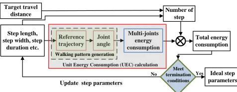
Due to the limited battery capacity, energy economy of locomotion becomes one of the chief requirements in making humanoids practical [1]. Therefore, the energetic cost for bipedal walking should be seriously taken into consideration. Many methods have been used to improve energy effi-ciency, such as compliant actuation design [2], [3], human walking learning [4], and gait parameters optimization [5], [6]. Generally, optimization-based approaches first evaluate a set of nominal step parameters and then update them following the gradient that minimizes the energetic cost of a desired travel distance. As shown in Fig. 1, the total energetic cost is actually determined by the Unit Energy Consumption (UEC) of one walking cycle.

As can be seen from Fig. 1, the first key procedure for energy efficiency optimization is to evaluate the UEC. As a prerequisite, an function for energy efficiency evaluation should be defined, which should not only be able to reflect the actual energy performance, but also be computed fast enough for its practical use. The joint power (calculated by multiplying joint torque by its angular velocity or motor

This work is supported by National Natural Science Foundation of China (Grant No. 51675385) and European Union’s Horizon 2020 robotics program CogIMon (ICT-23-2014, 644727).

1_{School of Power and Mechanical Engineering, Wuhan}

Univer-sity, Wuhan, Hubei Province, P. R. China 430072. {jtding,

xhxiao}@whu.edu.cn.

2_{Humanoid and Human Centered Mechatronics Research Line,}

Is-tituto Italiano di Tecnologia, via Morego, 30, Genova, Italy 16163.

[email protected].

Yes

Update step parameters

No Ideal step parameters

Meet termination

conditions

Joint angle Step length,

step width, step duration etc.

Reference trajectory

Multi-joints energy consumption

Total energy consumption

Unit Energy Consumption (UEC) calculation

Target travel

distance Number of

step

[image:2.612.315.553.160.253.2]

Walking pattern generation

Fig. 1: Flowchart for energetic cost optimization.

electric current by voltage) has been used widely as the measurement criteria (called joint power index, JPI). Al-though other simplified criteria have been used, such as the input torque used in [7] and [8] and input energy of hip actuators used in [9], they belong in nature to theJPIfamily. Since it requires obtaining joint angles and torques (using the inverse kinematics and dynamics) or electric data in advance, theJPIis hard to be used to generate the reference Center of Mass (CoM) trajectory directly, especially for complex multi-joints humanoid robots. In this paper, we aim to propose a novel optimal index for energetic cost evaluation, capable of generating walking patterns without requiring time-consuming iterative optimization.

Using the Linear Inverted Pendulum Model (LIPM), which is mass-concentrated, as the reference model that describes walking dynamics [10], the energy performance of the walk-ing system depends on the movement of the point mass, that is, the reference CoM trajectory. Although researchers have focused on the CoM motion optimization from different perspectives, such as boundary analysis [11]–[13] and Model Predictive Control (MPC) [14]–[16], most of them did not associate it with energy performance explicitly. Although the work in [17] has utilized CoM work to describe the actual energy consumption, the CoM work model was obtained via a very large number of physical simulations instead of deriving the mathematical expression. Herein, as the first main contribution, we derive the equivalent expression

of UEC and propose the CoM-Acceleration-based Optimal

Index (CAOI) for energy performance evaluation.

Humans naturally walk in an energy-efficient manner with heel-to-toe Zero Moment Point (ZMP) movement [18], [19].

To reduce the UEC with guaranteeing stability, allowable

in Double Support Phase (DSP), thus led to behaviours with improved energy efficiency by exploiting AZR. Nevertheless, the studies above did not provide the theoretical explanation as to why the ZMP movement in AZR would result in higher energy efficiency. That is to say, out of the above approaches, it is hard to tell which is the most efficient form of reference ZMP and why.

Besides, another effective way of energy saving is the use of the body vertical motion (CoM height variation, CoMHV), which has been demonstrated in [23] and [24]. Recent years have also seen efforts in bipedal walking with time-varying CoM height or straight leg [25], [26]. Using the CoMHV approach, above works qualitatively analyzed the energy efficiency (evaluated with the amount of torque input required by the knee joint). However, they still cannot provide an explicit proof of its energetic benefit. Thus, as another main contribution, we propose an analytic approach (as an example) for finding CAOI-optimal CoM trajectories and provide a unified proof of the energetic benefits of AZR and CoMHV.

The rest of this paper is organized as follows. In Section II, using the LIPM, the energetic cost of bipedal walking

is analyzed and the CAOI is derived. In Section III, an

analytic solution for generating the optimal CoM trajectory is proposed. Section IV analyzes the energetic benefits of AZR and CoMHV. In Section V, the energetic benefits of the proposed method are demonstrated on Nao-H25 humanoid robot. Section VI draws the conclusions.

II. ENERGYCONSUMPTION OFBIPEDALWALKING

A. Equations of Motion - LIPM

The LIPM, as a linear approximation of humanoid walking dynamics, is based on following assumptions: 1) the robot has a lumped mass body; 2) legs are massless and telescopic. Assuming no torque input at the support, the constant orbital energy is derived to describe the motion [10],

1 2γ˙

2₋ω2

2 γ

2_≡E

orbit, (1)

where, the letter γ denotes either the forward (x- axis) and lateral (y- axis) CoM displacement, ω is the natural frequency.

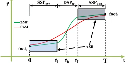
Herein, we define the Walking Cycle with Unit Energy

(UEWC) as shown in Fig. 2. Different from the natural

waking cycle consisting of one complete DSP and one

SSP, the UEWC consists of one pre-half SSP (SSPpre),

one transitional DSP (DSPtr), and another post-half SSP

(SSPpost). Thus, combined with (1), it is easy to find that the

robot speeds up in SSPpre while speeds down in SSPpost.

Also, it is easy to control the robot to speed up during the first half ofDSPtr and then to speed down during the latter

half of DSPtr. As the result, considering the directions of

CoM acceleration and CoM speed, they have the same sign (they are both positive) for t in [0, th) while the opposite

signs (positive velocity while decelerating) for t in (th, T].

Besides, at t=th, the velocity has its highest value, but the

acceleration is at the inflexion point (acceleration is going

SSPpre DSPtr SSPpost

DSP SSP

Natural waking cycle

Unit energy waking cycle

[image:3.612.327.541.48.190.2]

0

t

h

t

i

t

f

T

Fig. 2: LIPM motion during oneUEWC, SSPpre ends at time ti,

SSPpostbegins at timetf,T is the time duration of oneUEWC.

ZMP CoM

t footi

footf SSPpre DSPtr SSPpost

AZR

0 ti th tf T

Fig. 3: Linear reference ZMP and corresponding CoM trajectory during oneUEWC: the motion is along eitherx- ory- axis.

from positive to negative, and therefore it is zero at this point). That is,

  

  ¨

γtγ˙t>0, 0< t < th, ¨

γtγ˙t= 0, t=th, ¨

γtγ˙t<0, th< t < T ,

(2)

where,th= (ti+tf)/2.

Considering the ground reaction force, the ZMP dynamics of LIPM with constant height are given by

¨

γ=ω2(γ−Pγ), (3)

where,Pγ denotes the ZMP trajectory alongx- ory- axis. With (3), when ZMP falls behind CoM, the robot would speed up. Otherwise, it would speed down. WhenPγis fixed at the support, the CoM acceleration would meet (2) strictly. With linear or other forms of reference ZMP, (3) may not be satisfied at a particular period. However, studies reveal that this stage merely lasts for a short time when CoM velocity is also very low [13], [20]. Thus, it has little impact on the overall energy performance, as will be shown in following sections. Therefore, it is reasonable to assume (2) during the

whole UEWC. One example of the LIPM motion under a

linear ZMP trajectory during SSP is shown in Fig. 3.

B. Energy Consumption Evaluation during One UEWC

[image:3.612.328.545.237.347.2]

driven by conservative gravitational force, only the energy input for CoM movement in the horizontal plane needs to be considered. In this case, the direction of the input force either coincides with the speed direction or not. Thus, with assuming unit mass, we have

Enom= Z T

0

|Ftγ˙t|dt=

Z T

0

|γ¨tγ˙t|dt, (4)

where,Ft denotes the force acting on the lumped mass. Using (2), (4) can be simplified as following integral form:

Eint= Z th

0

¨ γtγ˙tdt−

Z T

th ¨ γtγ˙tdt

= 1 2([( ˙γth)

2_{−( ˙γ}

0)2] + [( ˙γth)

2_{−( ˙γ}

T)

2_]).

(5)

Using (2), for time t < th, the CoM velocity increases

monotonically. Otherwise, it decreases. Then, we can draw the following reasonable inferences

|γ˙th|>>|γ˙0|, |γ˙th|>>|γ˙T|. (6)

Then, the optimization of (5) can be further simplified as

JE= min 

 Z th

0

¨ γtdt

2 +

Z T

th ¨ γtdt

!2

. (7)

Finally, theCAOIfor energetic cost evaluation is proposed as

JC= min "

Z T

0

(¨γt)T(¨γt)dt

#

. (8)

Since the nominal energetic cost (Enom in (4)), integral

energetic cost (Eint in (5)), and the CAOI (JC in (8)) can

be calculated by merely employing CoM trajectory, we can evaluate the energy performance of bipedal walking without a need of computing joint angles. The effectiveness will be demonstrated in following sections.

III. ANALYTICSOLUTION OFCOM TRAJECTORY

Several previous studies such as [15], [16], [27] have taken the CoM acceleration as the control input and obtained robust walking patterns. However, these methods did not focus on the energy saving. According to the last section, any walking pattern generator, which minimizes the (8), can be used to generate the energy-efficient walking pattern. In term of boundary analysis, Lanari et al realized optimal double suppor transition with minimizing the CoM accel-eration during one walking cycle in [13] . However, they did not study the relationship between CoM acceleration and energy consumption. Besides, their methods can not deal with the reference ZMP trajectory determined by high order polynomial. In this paper, we address these problem and use the modified approach to obtain energetically efficient CoM trajectories.

A. Problem Statement

Taking into consideration the unstable component (xu) and

stable component (xs) as defined in [11] and [28], we have,

" ˙ xu ˙ xs # = ω 0

0 −ω xu xs + −ω ω

Pγ. (9)

Thus, the problem is, after defining the reference ZMP

during SSPpre and SSPpost, to solve the optimal CoM

trajectory with minimal energetic cost. According to [12],

to track a reference ZMP, the following bounded particular solutions exist:        x∗ u =ω

Z ∞

0

e−_ωτ

Pγ(t+τ)dτ,

x∗ s =ω

Z ∞

0

e−_ωτ

Pγ(t−τ)dτ.

(10)

Defining the deviations ofeu andes as

(

eu=xu−x ∗ u, es=xs−x

∗ s.

(11)

Then, the CoM trajectory can be solved by

γ=1

2(xu+xs) =γ ∗

+1

2(eu+es). (12)

After choosing the reference ZMP, theγ∗

can be calculated using (10) and the optimal CoM is determined byeuandes.

B. ZMP Tracking during SSP

During theSSPpre, we have the final condition att=ti. The error dynamics is solved as

" eu(t) es(t) #

=

e−ω(ti−t) ₀

0 eω(ti−t)

eu(ti)

es(ti)

. (13)

Considering following final conditiones(ti)≡0, the CoM trajectory from (12) can be given as

γt=

1 2e

−ω(ti−t)_[xu(t i)−x

∗

u(ti)] +γ

∗

t. (14)

Then, the CoM acceleration can be rewritten as

¨ γpret =

ω2

2 [eu(t) +es(t)] +ω

2_[γ∗

t −Pγ(t)]

=ω

2

2 eu(t) +ω

2_[γ∗

t −Pγ(t)].

(15)

Without loss of generality, the reference ZMPs during

SSPpre andSSPpost is given by polynomials as

Pγ = n

X

i=0

αiti. (16)

To make full use of AZR, we setnnot more than 2, which is the first extension compared with [13] which can only deal withnnot more than 1. In this case, we have

γ∗

t −Pγ(t) =

2αi 2

ω2 , (17)

where,αi

Finally, we can calculate the optimal quadratic index as

Jpre= Z ti

0

(¨γt)T(¨γt)dt=

Z ti

0

_ω2

2 e

−ω(ti−t)_eu(t i)+2αi2

2 dt

=ω

3

8(1−e

−2ωti_)[eu(t

i)]2+2αi2ω(1−e

−ωti_)eu(t i)+∆pre

=W1[eu(ti)]2−2H1eu(ti) + ∆pre,

(18) where,W1andH1 are the coefficients,∆pre is the constant term during theSSPpre.

Since the lower bound is0 rather than−∞, the integral

expression in(18)exists, which is the second extension. DenotingΨ = [xu(ti), xs(tf)]T,Fpre= [x∗u(ti), x∗s(ti)]T,

Jpre= ΨT

W1 0

0 0

Ψ−2ΨT

W1 0

0 0

F_pre+

H1

0

+∆pre

= ΨT_WpreΨ−2ΨT_H

pre+ ∆pre.

(19) Similarly, during theSSPpost, we have

Jpost= Z T

tf

(¨γt)T(¨γt)dt

= ω

3

8 (1−e

−2ω(T−_tf)_{) [es(t} f)]2

+ 2α2fω(1−e

−ω(T−_tf)_)es(t

f) + ∆post

=W2[es(tf)]2−2H2es(tf) + ∆post,

(20)

where,αf2 denotes the quadratic coefficient for theSSPpost, ∆post is the constant term during theSSPpost.

DenotingF_{post= [x}∗

u(tf), x∗s(tf)]T, (20) is rewritten as

Jpost=ΨT

0 0 0 W2

Ψ−2ΨT

0 0 0 W2

F_post+

0 H2

+∆post

=ΨTW_postΨ−2ΨTH_{post+ ∆post.}

(21)

C. Optimal CoM Trajectory duringDSPtr

To minimize the CAOI, following quadratic cost used in [13] during theDSPtr is also utilized here,

Jtr= Z tf

ti

(¨γt)T(¨γt)dt. (22)

Then, (22) can be solved by using optimal control theory. To be brief, we directly give the solution as

Jtr= ΨTH2TG −1_H

2Ψ + 2ΨTH2TG −1_H

1TFtr+ ∆tr = ΨTW_trΨ−2ΨTH_{tr+ ∆tr.}

(23) where,∆tr is the constant term during theDSPtr,

G= 1

3(tf−ti)

3 1

2(tf−ti)

2

1

2(tf−ti)

2 _t

f −ti

.

D. Optimal Solution during the Whole UEWC

Global optimal index can be givens as

JC=Jpre+Jtr+Jpost

= ΨTW_Ψ−2ΨTH_{+ ∆,} (24)

TABLE I: Basic parameters

Symbol Description Value

mc Robot’s mass 5.4 kg

lb Link length from hip to the center of body 50 mm

whip Hip width 85 mm

lth Link length from hip to knee 100 mm lsh Link length from knee to ankle 103 mm lank Link length from ankle to foot plane 45 mm

Zc Fixed height of LIPM 310 mm

dt Sampling time 0.01 s

T Time duration of oneUEWC 1.5 s

W Step width 100 mm

L Step length 60 mm

where, W ₌W_pre+W_tr+W_post,H ₌ H_pre+H_tr+H_post, ∆ = ∆pre+∆tr+∆post.

Therefore, the optimal value to minimize the energetic cost

of oneUEWC can be given by

Ψ =W−1_H.

(25)

IV. SIMULATIONRESULTS

A Nao-H25 robot containing 5 joints in each leg link is used with basic parameters listed in Table I. Using the proposed method, we first analyze the energy performance with employing AZR. Then, after extending the approach, the energetic benefit of CoMHV is demonstrated.

A. Bipedal Walking Using AZR

Three forms of ZMP trajectories including instantaneous changes between constant values, constant during SSP with

DSPtrand line trajectory during SSP withDSPtr, have been

studied in previous work. Herein, we proposed a parabolic ZMP trajectory to further exploit the AZR. In this paper, we assumed rectangular AZR with 40mm width and 40mm length. The time duration ofDSPtr (Tdsp), if existed, was

set to be 0.21s.

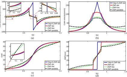
1) Reference trajectories: Using the analytic approach

proposed in Section III, the CoM accelerations, CoM ve-locities, CoM trajectories and ZMP trajectories within one

UEWC can be seen in Fig. 4.

Seen from the partial enlargement (A) in Fig. 4 (a), (2) was strictly satisfied when using the first three reference ZMP trajectories. In addition, observing Fig. 4 (b), the velocities at the initial and end time are much less than that at the half time, thus the (6) were also satisfied. Using the parabolic reference ZMP, (2) was not satisfied in specific time periods as seen in Fig. 4 (a). However, this stage merely lasted for a very short time and the CoM velocity during this period was also very low. Thus, the derivation process of the optimal evaluation index in Section II is reasonable.

(a) (b)

(c) (d)

0 0.5 1 1.5

-1000 -500 0 500 1000

t(s)

C

o

M

-a

cce

le

ra

tio

n

(m

m

/s

2)

Tdsp=0,ZMP-dot ZMP-dot ZMP-line ZMP-parabola 0 0.1 0.2

-30 0 30 60

0.7 0.75 0.8 0.85 -100

-50 0 50

A

B

0 0.5 1 1.5

0 50 100 150

t(s)

C

o

M

-ve

lo

ci

ty(

m

m

/s)

Tdsp=0,ZMP-dot ZMP-dot ZMP-line ZMP-parabola

0 0.5 1 1.5

0 10 20 30 40 50 60

t(s)

C

o

M

Tdsp=0,ZMP-dot ZMP-dot ZMP-line ZMP-parabola 0 0.1 0.2

0 2 4

0 0.5 1 1.5

0 10 20 30 40 50 60

t(s)

Z

M

P

(m

m

)

[image:6.612.99.520.56.313.2]

Tdsp=0,ZMP-dot ZMP-dot ZMP-line ZMP-parabola

[image:6.612.324.542.382.465.2]

Fig. 4: Trajectories generation under different reference ZMP trajectories, (a) CoM acceleration, (b) CoM velocity, (c) CoM trajectory, (d) ZMP trajectory; Tdsp=0, ZMP-dot represents the reference ZMP with instantaneous changes, ZMP-dot represents the constant value during SSP, where n=0 in (16), ZMP-line represents the linear reference ZMP during SSP, where n=1, ZMP-parabola represents the parabolic reference ZMP during SSP, wheren=2.

TABLE II: Energetic cost using AZR under different reference ZMP trajectories

Reference J_C Ratio Enom Ratio Eint Ratio

ZMP 104

(%) (104

) (%) (104

) (%) 1 64.06 100 11.39 100 11.38 100 2 24.97 39.0 4.87 42.8 4.82 42.4 3 9.37 14.6 2.69 23.6 2.66 23.3 4 8.41 13.1 2.31 20.3 2.01 17.7

Furthermore, since the CoM during DSPtr is obtained

by using optimization without guaranteeing the continuity of ZMP, the discontinuity was not avoided when moving from SSPpre toDSPtr and fromDSPtr toSSPpost, which

is visible in Fig. 4 (d). Although the discontinuity should be avoided in natural walking, the ZMP trajectory remained within the support polygon and still guaranteed the stability.

2) Energy performance: As can be seen from in Table II,

the nominal energetic cost of parabolic reference decreases to be only 20.3% of that using dot reference withoutDSPtr

and the integral energy decreased to be only 17.7%.

B. Bipedal Walking Using CoMHV

1) Reference trajectories generation: Vertical body

mo-tion has been observed in human walking, which contributes to lower energy consumption [24]. Taking into account the CoM height variation, the ZMP dynamics are given by

Pγ=γ−

zγ¨ ¨

z+g. (26)

Zc

hmax

SSPpre DSPtr SSPpost

Fig. 5: LIPM motion with CoMHV: the vertical CoM motion depends merely on two parametersZcandhmax.

As shown in Fig. 5, we assumed the symmetric parabolic

reference CoM height trajectory during the SSPpre and

SSPpost, with constant acceleration. In addition, the velocity

at the peak was set to be zero. For instance, the boundaries forSSPpre are

  

 

z(0) =Zc+hmax/2, z(ti) =Zc−hmax/2,

˙

z(0) = 0.

(27)

Since the amplitude (hmax) is very low compared with the stable component of height (Zc), considering the symmetry

of CoM height during SSPpre and SSPpost, we merely

modified the natural frequency without changing the CoM height. Then, during the wholeUEWC, the modified natural frequency (ωm) becomes,

ω2

m= (g+ ¨z)/z= (g+ ¨z)/Zc. (28)

[image:6.612.64.289.407.469.2]

solve (26).

2) Energy performance: To be brief, only the parabolic

reference ZMP was used, with four reference height trajec-tories. Seen from Table IV, theCAOI, the nominal energetic cost, and the integral energetic cost with CoMHV were all reduced. Furthermore, the simulation demonstrated that the energy performance depends much on the average height (Zc), which implied that the energetic cost would be reduced

dramatically if walking with straight knees.

TABLE III: Energetic cost using CoMHV

Zc+hmax J_C Ratio Enom Ratio Eint Ratio

(mm, mm) 104

(%) (104

) (%) (104

) (%) 310+0 8.42 100 2.31 100 2.01 100 310+20 8.31 98.7 2.30 99.6 2.00 99.5 320+0 8.07 95.8 2.26 97.8 1.97 98.0 320+20 7.97 94.7 2.25 97.4 1.96 97.5

V. HARDWAREEXPERIMENTS

A. Experimental Setup

Using ′

python′

language, the time cost for each loop including inverse kinematics calculation is less than 6.5 ms on one 3.3GHz processor. Thus, the algorithm could be implemented in real time.

The actual electrical energy consumption of humanoids was calculated by integrating joint power (electric voltage multiplies by current) during the whole walking process. For hardware experiments, each group of parameters was repeatedly run for 5 times and the average value was used as the ultimate result.

B. Experimental Results

1) Bipedal walking with employing AZR: Without further

explanation, the parameters for hardware experiments were the same with Section IV. Besides, in this section, only the reference ZMP with DSPs was used.

At this stage, no feedback controller was utilized. As can be seen from Fig. 6, the actual ZMP fluctuated dramatically, especially in the lateral direction. However, the actual ZMP was kept to be within the support polygon formed by support feet thus guaranteed the walking stability.

The actual energy consumption is listed in Table IV. Similar to the simulations, the minimal energetic cost was also obtained when using the parabolic reference ZMP. Under this group of step parameters, the actual energetic cost using parabolic reference ZMP reduced to be 87.4% of that using dot reference. Therefore, the experiments demonstrated the energetic benefit of AZR. Together with Section IV, our experiments have also demonstrated the validity ofCAOIfor energetic cost evaluation.

2) Bipedal walking with CoMHV: Using the parabolic

reference ZMP, the Nao robot can also walk stably, with the energetic costs listed in Table V. Similar with the simulation results, the actual energy consumption was also reduced. We can seen that the actual energetic cost using the

320mm+20mm height trajectory reduced to be 82.3%, more

(a)

(b)

0 100 200 300 400 500 600

-100 -50 0 50 100

Forward displacement(mm)

L

a

te

ra

l d

isp

la

ce

m

e

n

t(

m

m

)

ZMP-ref ZMP-actual Foot location

0 100 200 300 400 500 600

-100 -50 0 50 100

Forward displacement(mm)

L

a

te

ra

l d

isp

la

ce

m

e

n

t(

m

m

)

[image:7.612.328.540.54.252.2]

CoM-ref CoM-actual Foot location

Fig. 6: Reference/actual trajectories of bipedal walking with using parabolic reference ZMP with fixed step length, the solid rectangles represent the left foot while dash-dot the right.

TABLE IV: Actual energetic cost using AZR under different reference ZMP

Reference ZMP Energy(J) Ratio(%) 2(dot) 117.8 100 3(line) 108.6 92.2 4(parabola) 103.0 87.4

efficient than the 94.7% of CAOI result. The reason is that the torque on knee joint decreased dramatically in this case, which can not be reflected inCAOI.

VI. CONCLUSIONS

In this paper, using the LIPM, we derive the energy consumption model of one unit walking cycle and propose a CoM-Acceleration-based Optimal Index. Unlike the widely used Joint-Power-based evaluation function, the proposed index does not require the computation of the joint angles or input torques in advance. Instead, it can be used to directly generate the energetically efficient CoM trajectory.

[image:7.612.66.289.193.254.2]

Using the proposed criteria, we introduce one analytic method for CoM trajectory solution. Then, we theoretically reveal the energetic benefit of exploiting allowable ZMP region. At the present, four forms of reference ZMP are studied and the optimal CoM trajectories are generated. Results confirm that the parabolic reference ZMP trajectory is significantly better than a linear reference in energy saving. After then, using an approximate solution of nonlinear ZMP dynamics, the energetic benefit of using body vertical motion is also demonstrated.

TABLE V: Actual energetic cost using different COMHV trajecto-ries under parabolic ZMP

Zc+hmax (mm,mm) 310+0 310+20 320+0 320+20 Energy(J) 103.0 95.2 88.1 84.8

[image:7.612.363.510.331.371.2]

At the present, we focus on minimizing the energy consumption during one unit step, without considering the feasible constraints, such as joint angle limits. Considering the feasibility constraints and other details such as DC motor gain constant and the mass distribution, reference ZMP tra-jectory and vertical body motion need further optimization to realize energy-efficient walking, which is our current work. Furthermore, we are confident that the CAOI can be easily used as one of the optimization terms of other objective functions in the future. By choosing an appropriate weight, the multi-object optimization for bipedal waking could be realized with guaranteeing the energy efficiency.

REFERENCES

[1] A. D. Kuo, “Choosing your steps carefully,”IEEE Robotics & Au-tomation Magazine, vol. 14, no. 2, pp. 18–29, 2007.

[2] W. Roozing, Z. Li, D. G. Caldwell, and N. G. Tsagarakis, “Design optimisation and control of compliant actuation arrangements in articulated robots for improved energy efficiency,”IEEE Robotics and Automation Letters, vol. 1, no. 2, pp. 1110–1117, 2016.

[3] A. Mazumdar, S. J. Spencer, C. Hobart, J. Salton, M. Quigley, T. Wu, S. Bertrand, J. Pratt, and S. P. Buerger, “Parallel elastic elements improve energy efficiency on the steppr bipedal walking robot,”

IEEE/ASME Transactions on Mechatronics, vol. 22, no. 2, pp. 898– 908, 2017.

[4] K. Sohn and P. Oh, “Applying human motion capture to design energy-efficient trajectories for miniature humanoids,” in IEEE/RSJ International Conference on Intelligent Robots and Systems, 2012, pp. 3425–3431.

[5] V.-H. Dau, C.-M. Chew, and A.-N. Poo, “Achieving energy-efficient bipedal walking trajectory through ga-based optimization of key pa-rameters,”International Journal of Humanoid Robotics, vol. 6, no. 04, pp. 609–629, 2009.

[6] E. Heijmink, A. Radulescu, B. Ponton, V. Barasuol, D. G. Caldwell, and C. Semini, “Learning optimal gait parameters and impedance pro-files for legged locomotion,” inIEEE-RAS International Conference on Humanoid Robotics, 2017, pp. 339–346.

[7] Z. Wang, G. Yan, Z. Lin, C. Tang, and S. Song, “A switching control strategy for energy efficient walking on uneven surfaces,”International Journal of Humanoid Robotics, vol. 12, no. 04, p. 1550015, 2015. [8] C. Choi and E. Frazzoli, “Torque efficient motion through singularity,”

inIEEE International Conference on Robotics and Automation, 2017, pp. 5012–5018.

[9] S. J. Hasaneini, C. J. Macnab, J. E. Bertram, and H. Leung, “Op-timal relative timing of stance push-off and swing leg retraction,” in

IEEE/RSJ International Conference on Intelligent Robots and Systems, 2013, pp. 3616–3623.

[10] S. Kajita, O. Matsumoto, and M. Saigo, “Real-time 3d walking pattern generation for a biped robot with telescopic legs,” in IEEE International Conference on Robotics and Automation, vol. 3, 2001, pp. 2299–2306.

[11] T. Takenaka, T. Matsumoto, and T. Yoshiike, “Real time motion generation and control for biped robot-1 st report: Walking gait pat-tern generation,” inIEEE/RSJ International Conference on Intelligent Robots and Systems, 2009, pp. 1084–1091.

[12] L. Lanari, S. Hutchinson, and L. Marchionni, “Boundedness issues in planning of locomotion trajectories for biped robots,” in IEEE-RAS International Conference on Humanoid Robots, 2014, pp. 951–958. [13] L. Lanari and S. Hutchinson, “Optimal double support zero moment

point trajectories for bipedal locomotion,” inIEEE/RSJ International Conference on Intelligent Robots and Systems, 2016, pp. 5162–5168. [14] J. Casta˜no, A. Hernandez, Z. Li, C. Zhou, N. Tsagarakis, D. Caldwell, and R. De Keyser, “Implementation of Robust EPSAC on dynamic walking of COMAN Humanoid,” in19th World Congress: The Inter-national Federation of Automatic Control, 2014, pp. 8384–8390. [15] S. Caron and A. Kheddar, “Multi-contact walking pattern generation

based on model preview control of 3D CoM accelerations,” in

IEEE-RAS International Conference on Humanoid Robots, 2016, pp. 550–

557.

[16] M. Naveau, M. Kudruss, O. Stasse, C. Kirches, K. Mombaur, and P. Sou`eres, “A reactive walking pattern generator based on nonlinear model predictive control,” IEEE Robotics and Automation Letters, vol. 2, no. 1, pp. 10–17, 2017.

[17] M. Brandao, K. Hashimoto, J. Santos-Victor, and A. Takanishi, “Foot-step planning for slippery and slanted terrain using human-inspired models.”IEEE Transactions on Robotics, vol. 32, no. 4, pp. 868–879, 2016.

[18] C. Zhou, X. Wang, Z. Li, and N. Tsagarakis, “Overview of Gait Synthesis for the Humanoid COMAN,”Journal of Bionic Engineering, vol. 14, no. 1, pp. 15–25, 2017.

[19] H. Zhu, M. Luo, T. Mei, J. Zhao, T. Li, and F. Guo, “Energy-efficient bio-inspired gait planning and control for biped robot based on human locomotion analysis,”Journal of Bionic Engineering, vol. 13, no. 2, pp. 271–282, 2016.

[20] K. Erbatur and O. Kurt, “Natural zmp trajectories for biped robot reference generation,” IEEE Transactions on Industrial Electronics, vol. 56, no. 3, pp. 835–845, 2009.

[21] T.-H. S. Li, Y.-T. Su, S.-H. Liu, J.-J. Hu, and C.-C. Chen, “Dynamic balance control for biped robot walking using sensor fusion, kalman filter, and fuzzy logic,”IEEE Transactions on Industrial Electronics, vol. 59, no. 11, pp. 4394–4408, 2012.

[22] H.-K. Shin and B. K. Kim, “Energy-efficient gait planning and control for biped robots utilizing the allowable zmp region,” IEEE Transactions on Robotics, vol. 30, no. 4, pp. 986–993, 2014. [23] ——, “Energy-efficient gait planning and control for biped robots

utilizing vertical body motion and allowable zmp region,” IEEE Transactions on Industrial Electronics, vol. 62, no. 4, pp. 2277–2286, 2015.

[24] Y. Ogura, K. Shimomura, H. Kondo, A. Morishima, T. Okubo, S. Momoki, H.-o. Lim, and A. Takanishi, “Human-like walking with knee stretched, heel-contact and toe-off motion by a humanoid robot,” in IEEE/RSJ International Conference on Intelligent Robots and Systems, 2006, pp. 3976–3981.

[25] S. Kajita, M. Benallegue, R. Cisneros, T. Sakaguchi, S. Nakaoka, M. Morisawa, K. Kaneko, and F. Kanehiro, “Biped walking pattern generation based on spatially quantized dynamics,” in IEEE-RAS International Conference on Humanoid Robotics, 2017, pp. 599–605. [26] Y. You, S. Xin, C. Zhou, and N. Tsagarakis, “Straight Leg Walking Strategy for Torque-controlled Humanoid Robots,” inIEEE Interna-tional Conference on Robotics and Biomimetics, 2016, pp. 2014–2019. [27] C. Brasseur, A. Sherikov, C. Collette, D. Dimitrov, and P.-B. Wieber, “A robust linear mpc approach to online generation of 3d biped walking motion,” inIEEE-RAS International Conference on Humanoid Robots, 2015, pp. 595–601.

[28] J. Englsberger, C. Ott, and A. Albu-Sch¨affer, “Three-dimensional bipedal walking control based on divergent component of motion,”