White Rose Research Online URL for this paper: http://eprints.whiterose.ac.uk/102528/
Version: Accepted Version
Article:
Dou, Q, Wei, L, Magee, D et al. (1 more author) (2017) Real-Time Hyperbolae Recognition and Fitting in GPR Data. IEEE Transactions on Geoscience and Remote Sensing, 55 (1). pp. 51-62. ISSN 0196-2892
https://doi.org/10.1109/TGRS.2016.2592679
(c) 2016 IEEE. Personal use of this material is permitted. Permission from IEEE must be obtained for all other users, including reprinting/ republishing this material for advertising or promotional purposes, creating new collective works for resale or redistribution to servers or lists, or reuse of any copyrighted components of this work in other works
[email protected] https://eprints.whiterose.ac.uk/ Reuse
Unless indicated otherwise, fulltext items are protected by copyright with all rights reserved. The copyright exception in section 29 of the Copyright, Designs and Patents Act 1988 allows the making of a single copy solely for the purpose of non-commercial research or private study within the limits of fair dealing. The publisher or other rights-holder may allow further reproduction and re-use of this version - refer to the White Rose Research Online record for this item. Where records identify the publisher as the copyright holder, users can verify any specific terms of use on the publisher’s website.
Takedown
If you consider content in White Rose Research Online to be in breach of UK law, please notify us by
Real Time Hyperbolae Recognition
and Fitting in GPR Data
Qingxu Dou, Lijun Wei, Derek R. Magee, and Anthony G. Cohn
Abstract—The problem of automatically recognising and fitting hyperbolae from Ground Penetrating Radar (GPR) images is addressed, and a novel technique com-putationally suitable for real time on-site application is proposed. After pre-processing of the input GPR images, a novel thresholding method is applied to separate the regions of interest from background. A novel column-connection clustering (C3) algorithm is then applied to separate the regions of interest from each other. Subse-quently, a machine learnt model is applied to identify hyperbolic signatures from outputs of the C3 algorithm and a hyperbola is fitted to each such signature with an orthogonal distance hyperbola fitting algorithm. The novel clustering algorithm C3 is a central component of the proposed system, which enables the identification of hyperbolic signatures and hyperbola fitting. Only two features are used in the machine learning algorithm, which is easy to train using a small set of training data. An orthogonal distance hyperbola fitting algorithm for ‘south-opening’ hyperbolae is introduced in this work, which is more robust and accurate than algebraic hyperbola fitting algorithms. The proposed method can successfully recognise and fit hyperbolic signatures with intersections with others, hyperbolic signatures with distortions and incomplete hyperbolic signatures with one leg fully or largely missed. As an additional novel contribution, formu-lae to compute an initial ‘south-opening’ hyperbola directly from a set of given points are derived, which make the system more efficient. The parameters obtained by fitting hyperbolae to hyperbolic signatures are very important features, they can be used to estimate the location, size of the related target objects, and the average propagation velocity of the electromagnetic wave in the medium. The effectiveness of the proposed system is tested on both synthetic and real GPR data.
Index Terms—GPR, Column-connection clustering algo-rithm, hyperbola recognition, orthogonal distance fitting, machine learning, buried asset detection.
I. INTRODUCTION
The authors are with the School of Computing, University of Leeds, Leeds, UK, LS2 9JT. email: [email protected] (cor-responding author), [email protected], [email protected], [email protected]; t: +44 (0)113 343 5430; f: +44 (0)113 343 5468.
A
S a non-destructive tool for investigation of shallow subsurface, GPR has been widely used in detection and mapping of subsurface utilities such as pipes and cables [1]. There are typically two pattern shapes in B-scan images of GPR, hyperbolic curves and linear segments [2]. Hyperbolic curves are due to objects with a cross-section size of the order of the radar pulse wavelength; linear segments stem from planar interfaces between layers with different electrical impedance. Because of system noise, the heterogeneity of the medium and mutual wave interactions, GPR images are usually noisy. It is a complex task to automatically extract hyperbo-lae from GPR data. Considerable research has been devoted in this area and many different strategies have been employed to tackle this topic e.g. [3]– [11]. In addition, if the parameters of a hyperbolic signature can be obtained by fitting a hyperbola to it, the parameters can be used to estimate the location and size of the related target object, and the average propagation velocity of the electromagnetic wave in the medium [12].suitable for very clean GPR images. Otherwise, it would be very difficult to group the points detected from a certain edge for fitting. In [10], an edge detector is also applied to detect edges from GPR images. Although this method can be applied on complex GPR images, in fact, no fitting is applied directly on the detected edge points so only the apexes of the hyperbolae are detected and other parameters of the related hyperbolae are missed, which are essential for identifying other properties of the utilities such as the size of the utilities [12] and even the materials of the utilities [11].
[image:3.612.325.550.57.190.2]Another type of approach uses machine learning methods to narrow down the regions including hy-perbolae in the first step and then a fitting method is applied to find the hyperbola parameters [9], [18]. In [18], after the regions including hyperbolae are extracted with a neural network, an edge detector is employed to detect edges in the extracted regions and then the parameters of hyperbolae are extracted through a generalized Hough transform. In [9], the Viola-Jones algorithm [19] is employed to extract the regions believed to contain hyperbolae, followed by a generalized Hough transform fitting based on the detected edge points. The disadvantages of ex-tracting hyperbola parameters through a generalized Hough transform and edge fitting are pointed out above. In addition, as pointed out by the authors of [9], the quality of detection results depends strongly on the quality and size of the available data for train-ing. The experimental statistics are very impressive with respect to recall and precision for hyperbolae detection and fitting in [7], but the algorithm is only tested with synthetic data generated with GprMax [20] and the scenarios are relatively simple such as no intersection of the hyperbolic signatures is seen in the displayed GPR images. In [21], the authors suggest a probabilistic hyperbola mixture model based on a classification expectation maximization algorithm to extract multiple hyperbolae from a GPR image in one go. There are at least two issues worthy for further consideration. First, compared with an orthogonal circle or ellipse fitting algorithm, orthogonal hyperbola fitting algorithms are more sensitive to the configuration of the given points. The expectation maximization algorithm starts with a general initial partition of the given points, it is difficult to guarantee the convergence of the hyperbola fitting algorithm. Second, the computa-tion of an orthogonal hyperbola fitting algorithm is
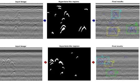
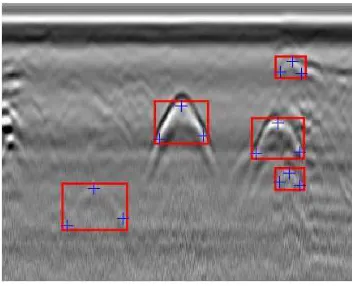
Fig. 1. Examples of difficult scenarios that can be tackled by the proposed hyperbola recognition and fitting method. The first column contains the input GPR images, the second column contains the candidate hyperbolic signatures, and the third column contains the fitted hyperbolae with difficult scenarios, including intersecting hyperbolae in rectangles 1, incomplete or distorted hyperbolae in
rectangles2andrectangles3.
expensive. In each step the expectation maximiza-tion algorithm calls the hyperbola fitting algorithm multiple times.
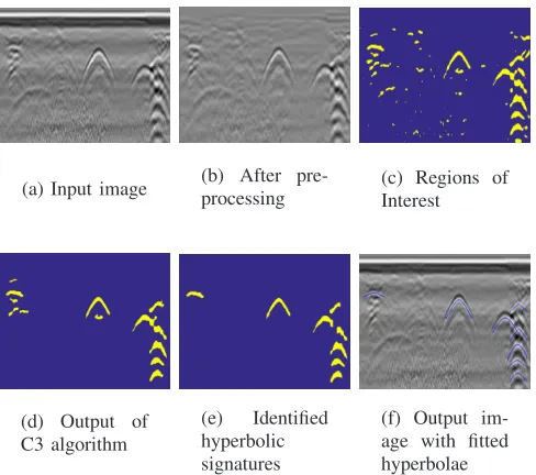
(a) Input image (b) After pre-processing
(c) Regions of Interest
(d) Output of C3 algorithm
(e) Identified hyperbolic signatures
[image:4.612.54.298.63.279.2](f) Output im-age with fitted hyperbolae
Fig. 2. An illustration of the application of the proposed technique on the bright regions (as described in Section II-A) of a real GPR image. In the first row, (a) the input image, (b) the image after preprocessing, (c) the regions of interest after thresholding. In the second row, (d) clusters after applying C3 algorithm, (e) identified hyperbolic signatures by applying the machine learning algorithm, (f) the output image from the system with fitted hyperbolae Intersecting(with crossing tails, connected without crossing tails), Distorted (asymmetric or incomplete) (best viewed in colour).
the corresponding parameters which can be used to estimate the location and size of the target object, and the signal propagation velocity in the medium [12].
The C3 algorithm is the central component of this work. The previous clustering algorithms are either based on the distance between points [22], [23] or the density of points within a certain area [24], [25]. They are not capable of separating connected regions or segmenting two hyperbola signatures with an intersection. The proposed C3 algorithm is based on matching sequences of elements in adjacent columns with the same row numbers. The output clusters of this algorithm include different combinations of connected blocks and one block can belong to multiple different clusters. With this algo-rithm, most hyperbolic signatures can be segmented from other regions even if they are connected or have intersections before clustering. Without this step, the proposed machine learning algorithm and hyperbola fitting algorithm can not be applied.
The hyperbola fitting algorithm is also a crucial component of this work. There is a large body of
conic fitting algorithms in the literature [26]–[30]. Compared to algebraic distance, orthogonal distance is invariant to transformations in Euclidean space, therefore orthogonal distance fitting algorithms are more robust and accurate than algebraic distance fitting algorithms [26]. In this work, we introduce a least-squares orthogonal distance fitting algorithm for ‘south-opening’ hyperbolae based on the work of [26]. The efficiency of the fitting algorithm makes this system suitable for real time on-site application. In addition, a novel way to compute the initial hyperbola parameters directly from the given points is introduced. Compared to using algebraic hyper-bola fitting results as the initial hyperhyper-bola for the orthogonal hyperbola fitting as in [26], [29], [31], the initial hyperbola computed with the proposed method is usually closer to the final fitted one, this makes the fitting algorithm even more efficient.
The rest of this paper is organised as follows. We present the proposed C3 algorithm and the related GPR image pre-processing schemes in section II, which is followed by a description of the machine learning algorithm for hyperbolic signatures iden-tification in section III. The orthogonal distance hyperbola fitting algorithm and the hyperbola ini-tialisation procedure are presented in Section IV. The experimental results are shown and analysed in Section V, and finally, conclusions are drawn in Section VI.
II. A COLUMN-CONNECTION CLUSTERING
ALGORITHM
In this section, we present the proposed column-connection clustering (C3) algorithm and the related pre-processing procedures on real data.
A. Adaptive Thresholding of the Input Images
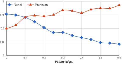
Fig. 3. The illustration of effect ofρbin Equation (1) on the values of recall and precision of hyperbola fitting when applying the proposed system on a group of GPR images. Recall = tp
tp+f n, precision = tp
tp+f p, wheretpis the number of correctly fitted hyperbolae by the algorithm,f nis the number of hyperbolae in the ground truth which are not correctly fitted by the proposed algorithm, and f p is the number of fitted hyperbolae not included in the ground truth.
eliminate the bright ground surface reflectance strip. An example image after the pre-processing is shown in Fig. 2 (b). The window size of the filter should not be too large but within a certain range, the experimental results are not that sensitive to it. In our experiments, we tried with3×3,5×5and7×7 (in pixels) and very similar results were obtained. The experimental results shown in this paper were done with filter window size of 3×3.
The regions corresponding to the maxima of positive phase (bright) or minima of negative phase (dark) of the reflected radar signal are the regions of interest for identifying hyperbolae. Since the dark regions of an image corresponding to the bright regions of its inverse image, in the following sections of this paper, we focus on the bright regions representing high responses. If a suitable threshold value can be selected to separate the regions of interest (high responses) from the background, it simplifies further processing. To pick a threshold to separate two regions with different intensities in an image, it is natural to use the intensity value of a pixel on the boundary between these two regions as the threshold. In our work, a large number of regions of interest need to be separated from the background and many boundaries between the regions of interest and the background are involved. We decide to pick a threshold, which relates to the average of the in-tensity values of the boundary points. First, an edge detector is used to extract the edges between regions of interest and the background to obtain the intensity values of the edge points. If we use the average of all
the edge points as the threshold, then experiments give good recall values but bad precision. If we average by chopping off some darker edge points, the balance between the value of recall and the value of precision improves. But if we chop off too many darker edge points before averaging, the balance worsens. So only the edge pixel intensities which are greater than a certain percentage of the value of the highest edge pixel intensity are used for averaging to obtain the threshold value. The computation of the threshold can be performed with the following expression:
thresholdb =mean{Ie|Ie > ρb×MaxIe} (1)
wheremeanis a function for computing the average among a set of values, Ie is the intensity value of an edge pixel, MaxIe is the highest edge intensity
value and ρb is a fraction (0< ρb <1).
The effect of the valueρb on the values of recall
and precision of fitted hyperbolae when applying the proposed system on a group of real GPR images is demonstrated in Fig. 3. It can be seen that with the value of ρb increasing, recall decreases while
precision increases. Balancing between these two factors, 0.1 is used in our experiments.
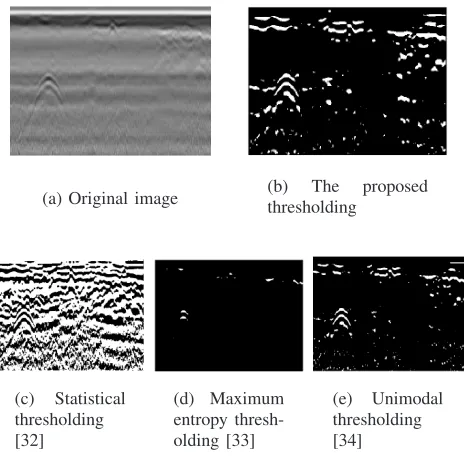
The proposed adaptive thresholding algorithm is also compared with other existing thresholding methods in the literature, which are totally different from each other: the statistical thresholding method in [32], the maximum entropy thresholding method in [33], and the unimodal thresholding method in [34]. The method proposed by Kapur et al in [33] was also used by [11] on GPR images to separate the hyperbola regions from the background. As can be seen in Figure 4(c), it seems that the threshold given by the statistical thresholding method in [32] is too low and it only removes those dark areas; and the threshold given by the maximum entropy thresholding method in [33] is usually too high to retain all the hyperbola regions (Figure 4(b)). The outputs from the unimodal thresholding method [34] (Figure 4(e)) are very similar to those of the proposed method (Figure 4(f)), although based on totally different computation strategies. Further comparison on these two methods with detailed statistics can be found in section V.
(a) Original image (b) The proposed thresholding
(c) Statistical thresholding [32]
(d) Maximum entropy thresh-olding [33]
[image:6.612.317.561.52.284.2](e) Unimodal thresholding [34]
Fig. 4. Comparison of different thresholding methods for bright regions on one real GPR image.
it is regarded as a point. On the other hand, if the value at a pixel is zero, it is regarded as background.
B. Column-connection Clustering (C3) Algorithm
After an input image is converted into a binary one by thresholding, the C3 algorithm is applied to separate the selected regions into different clusters. To explain the C3 algorithm clearly, two concepts should be clarified first: Column Segment and Con-necting Elements of two column segments from adjacent columns.
Column Segment:when searching along a column of a binary image, if the number consecutive points is equal to or higher than a pre-defined number s, then this group is called a column segment. For example, in Figure 5, if the value of s is defined as 4, then there are three column segments along column C1. The second group is not a column segment as there are only two consecutive elements in this group. The purpose of selecting a threshold s for column segments is for noise resistance. The criterion to choose it depends on the noise level of the sensor, the radar central frequency and the sampling frequency. Concretely, the maximum value ofsis proportional to the sampling frequencyfsand
inversely proportional to the radar frequencyfc. An
[image:6.612.60.293.63.292.2]ideal value of s should be bigger than most of the noise but lower than k·fs/fc (k is a constant) so
Fig. 5. An illustration of the C3 algorithm (see detailed explanation in the text).
as to reject most of the noise and remain the signal. In our experiments, the value of s is the same for different parts of the image.
Connecting Elements: The location of a point in a certain column segment is defined by its row num-ber. If we say two adjacent column segments have connecting elements, it means they have elements from the same row. In this work we only compare the elements between two column segments which are from adjacent columns. For example, in Figure 5, there are four connecting elements between the first column segments from column C1 and column C2.
situation, Cluster 2 extends to Column C2 and splits into two clusters Cluster 2a and Cluster 2b. All
the elements in Cluster 2 are associated with both clusters with the elements in the second column segment of Column C2 added to Cluster 2a and the
elements in the third column segment of ColumnC2 added to Cluster2b. As for the third column segment
in Column C1, since there is no connecting element in Column C2 with it, Cluster 3 stops at Column C1. The fourth column segment in Column C2 has four elements which is no less than s, and there is no connecting element in the previous Column C1, therefore a new cluster starts from Column C2 with the elements in the fourth column segment as the seeds.
This procedure is performed until the last column is scanned to obtain all the clusters based on col-umn connection. This algorithm is symmetric with respect to the scanning direction, i.e. there is no dif-ference in performing the scanning procedure from left to right or from right to left. The outputs of the clustering algorithm with one GPR image are shown in Figure 6 (b) and (c). For each output cluster from the C3 algorithm, a central string, which is the curve connecting the middle points of the elements in each column is computed as shown in Figure 6 (b). The central string is a very important feature in C3 algorithm, it is used for further segmentation, machine learning and hyperbola fitting. Physically, the calculated central string corresponds to the peak point of the reflected signal.
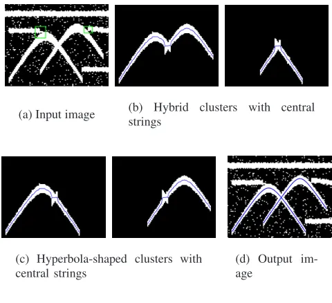
[image:7.612.317.557.63.282.2]The C3 clustering algorithm can separate hyper-bolic signatures with intersections. It can be seen in Figure 6, two hyperbolic signatures, which intersect each other, are separated by the C3 algorithm as displayed in Figure 6 (c). This example is based on synthetic data. In real GPR images, the intersec-tions between two hyperbolic signatures are more complicated. In some cases, due to the low strength of response, the parts below the intersection point are missed as the cluster shown within the rectangle window in Figure 7(a). In this situation, the C3 al-gorithm described so far can not separate them from each other. The whole region is usually identified as a non hyperbolic signature in the machine learning step and two hyperbolae are missed. To deal with this situation, the above mentioned C3 algorithm is extended with a further segmentation step.
Suppose the curve shown in Figure 7(b) is the central string of an output cluster from the first step
(a) Input image (b) Hybrid clusters with central strings
(c) Hyperbola-shaped clusters with central strings
(d) Output im-age
Fig. 6. The application of the proposed system on a synthetic data set. Some output clusters of the C3 algorithm with the central strings are displayed in (b) and (c). The fitted hyperbolae are shown in (d).
of the C3 algorithm. It is similar to the situation where two hyperbolae intersect each other at point P and the parts below point P are not detected. Mathematically, the first derivative at point P is 0 and the second derivative at point P is positive; pointP is detected by checking its first and second derivatives and the related cluster is broken at the column corresponding to pointP. In the final output of C3 fed to the machine learning algorithm (which will filter out non-hyperbolic shaped responses), the original cluster before this step is also included for avoiding misjudgements.
(a) After one step of C3
(b) A schematic
of two
connected hyperbolae
(c) After further segmentation
Fig. 7. Further segmentation on connected hyperbola signatures (best viewed in colour).
[image:7.612.316.561.535.667.2]the original image is noisy but the images of the separated clusters are clean. This is achieved with the help of pre-defined parameters. For a reasonable value ofssuch as 2or3, the number of the consec-utive noise points along a column is usually not as high as s. Therefore almost all the noisy points are eliminated in the clustering step. By tuning the value of s, the proposed algorithm can deal with images with different noise levels. We tried different values for parameter sin our experiments. The best results were obtained using s= 3. So we set s equal to 3 in the shown experimental results.
The pseudo-code of the proposed clustering algo-rithm can be presented as follows:
for i from min_column to max_column do if i==min_column
for j from 1 to num_col_seg_c do cell{j,1}=col_seg_c(j); end
else
for j from 1 to num_col_seg_c do record=zeros(1,num_col_seg_p); for k=1 to num_col_seg_p do
n=num_same_elements(col_seg_c(j), col_seg_p(k));
if n>=s && record(j)==0
cell{j,1}=[cell{j,1} col_seg_c(j)]; record(j)=1;
elseif n>=s && record(j)==1 kk=size(cell,1)+1; cell{kk,1}=cell{j};
cell{kk,1}=[cell{kk,1} col_seg_c(j)]; elseif n<s
kk=size(cell,1)+1; cell{kk,1}=col_seg_c(j); end
end end end end
For a cluster containing one hyperbolic signature, a hyperbola is fitted to this cluster to obtain its parameters. Which output clusters should be re-garded as a hyperbolic signature? We answer this question by a machine learnt model for identifying hyperbolic signatures, which is explained in the next section.
III. MACHINELEARNING ALGORITHM FOR
IDENTIFYING HYPERBOLIC SIGNATURES
In this section we present a machine learning method for identifying hyperbolic signatures.
A. Feature Extraction for A Neural Network Clas-sification Algorithm
In order to successfully identify hyperbolic sig-natures from the outputs of C3 algorithm, it is
Fig. 8. The first and second derivative curves of a south-opening hyperbola on a domain symmetric to the hyperbola centre. The marker points on each curve make up a template.
necessary to extract attributes that characterise hy-perbolic signatures and distinguish them from other undesired clusters and composite clusters of more than one hyperbola.
In a GPR image, the detected hyperbolae are manifested as ‘south-opening’ branches. The gen-eral equation of a ‘south-opening’ branch of a hyperbola is written as
(y−y0)2
a2 −
(x−x0)2
b2 = 1, with y < y0 (2) whereyandxrelate to the values along the vertical and horizontal axes, the vertical axis y is propor-tional to the two-way travel time of waves and the horizontal axisxis the distance along the measured direction. (x0, y0) is the centre of the hyperbola, a is the length of the semi-major axis and b is the length of semi-minor axis.
The first and second derivatives of the function expressed by equation (2) have the following form:
dy dx =−
a b
x−x0
p
(x−x0)2 +b2
(3)
d2 y dx2 =−
ab
((x−x0)2+b2)3/2
(4)
[image:8.612.363.512.55.163.2]normalized cross correlation (NCC) values. As a typical hyperbola of response from buried utilities, y2
/25−x2
/16 = 1is used as the pre-defined hyper-bola in all the experiments in this work. By testing with different hyperbolae, we found that there is no significant difference if other hyperbolae are used as the pre-defined template hyperbola because NCC is invariant to scaling and the shape of hyperbolae do not change significantly for small sized objects.
When x is discretized in a certain range, the re-lated first and second derivatives of the pre-defined hyperbola make up two vectors, which are used as templates to identify the hyperbolic signatures from the outputs of C3 algorithm. To use the templates, for each output cluster from the C3 algorithm, the central string is computed as shown in Figure 6 (b). NCC values of the first and second derivative values along each central string against the templates are computed after aligning the peaks of the central string and the pre-defined hyperbola curve. The NCC value of two vectors v1 and v2 is defined as follows:
ncc= |v1·v2| |v1| ∗ |v2|
(5)
When two ‘south-opening’ hyperbolae are aligned with respect to the x coordinates of their centres, the NCC values of their first and second derivative curves are high (close to 1).
The normalized cross correlation values of the first and second derivatives are used in the following neural network classification step to identify the hyperbolic signatures.
B. Neural Network Classification
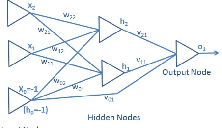
A group of positive and negative samples are selected manually from the outputs of C3 algorithm and the two NCC values of each sample are com-puted, which are used to train a neural network clas-sifier. This stage provides the subsequent stages with a continuous measure of confidence as to whether a particular output of theC3is a hyperbolic signature or not. First, a three-layer feed-forward perceptron neural network (as in Figure 9) was trained with the backpropagation learning algorithm [35] and the corresponding vectors were recorded. The trained neural network can be applied to classify the outputs of C3algorithms new to the neural network.
[image:9.612.326.552.60.190.2]In practice, a smoothed version of the central string is used when comparing with the templates.
Fig. 9. Neural network diagram.
Judged by the experimental results below in sec-tion V, the proposed neural network classificasec-tion algorithm works very well for most hyperbolic signatures.
IV. ORTHOGONAL DISTANCE HYPERBOLA
FITTING
In this section, we present a robust orthogonal distance fitting algorithm for hyperbola fitting [26] and introduce a method to initialize a hyperbola directly from given points.
A. The Hyperbola Fitting Algorithm
Given a set of points (xi, yi)mi=1, the orthogonal distance di of a point Pi = (xi, yi) to a hyperbola
can be expressed by
d2
i = min
φi
[(xi−x(φi))2+ (yi−y(φi))2] (6)
where (x(φi), y(φi)) is the corresponding closest
point of Pi on the hyperbola.
The task is to determine a, b, x0 and y0 for this hyperbola by solving
argmina,b,x0,y0
m
X
i=1 d2
i (7)
It is not a trivial task to find the closest point of Pi on a hyperbola when Pi itself is not on this
hyperbola as explained below. Suppose P(x, y) is the closest point of Pi on the hyperbola expressed
by Equation (2). Since the connecting line of P and Pi is perpendicular to the tangent line of the
Fig. 10. An example of hyperbola fitting with a synthetic data set.
dy dx ·
yi−y
xi−x
= a
2
(x−x0) b2(y−y
0)
· yi−y
xi−x
=−1 (8)
The coordinates of P can be obtained by solving the system of equations (2) and (8) with a gener-alized Newton method. The average time needed for finding the closest point of a given point on a hyperbola is about 0.0015 seconds using a computer with Intel 3.6GHz processor coded in Matlab.
After finding the closest pointP on the hyperbola for each given point Pi, the coefficients of the
hyperbola satisfying Equation (7) can be obtained by using Gauss-Newton iteration
J·∆c= ∆P (9)
ck+1 =ck+λ∆c (10)
where c = [a, b, x0, y0]t are the parameters of
the current hyperbola, ∆P = |P−Pi| with Pi = [xi, yi]t, a given point, and P = [x, y]t, the closest
corresponding point of Pion the current hyperbola.
J = ∂F
∂c|ck is the Jacobian matrix with F as the
corresponding expression of the current hyperbola and λ is the step size parameter.
B. Direct Hyperbola Initialization
In previous work on orthogonal distance fitting, some authors suggest to take the initial parameter values from the corresponding algebraic distance fitting [26], [29]. In this work, because of the robustness of the fitting algorithm and the fact that we only deal with the south-opening branch of a hyperbola from GPR data, we propose a simple and fully automatic procedure to directly compute the parameters of the initial hyperbola which works
very well for converging to the global minimum of Equation 7 in our experiments.
To determine a south-opening branch of a hy-perbola, if its apex is given, only two other points, which satisfy certain constraints, are needed.
Given (xv, yv) as the coordinates of the apex of
a south-opening branch of a hyperbola and (xl, yl)
as a point on the left hand side of line x = xv
and (xr, yr) as a point on the right hand side of
the line x = xv, what constraints must be satisfied
to determine a hyperbola? Obviously, the following two constraints should be satisfied first: yv > yl and
yv > yr. Second, (xl, yl) and (xr, yr) can not be
symmetric to the line ofx=xv. The reason will be
given later in this section. Third, whenxv, yv, xl,yl
andxr are fixed values, the value of yr must satisfy
Equations (11) and (12).
yr < yv+
(xv−xr)·(yv−yl)
xv−xl
(11)
yr>
sl·yv −sr·(yv−yl)
sl
(12)
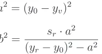
where sr = (xr−xv)2 and sl = (xl−xv)2.
For a given set of points (xi, yi)mi=1 for fitting a south-opening hyperbola, to initialize a hyperbola, we first compute three points from the given points. First, the point with largest y-coordinate is found and a centroid is computed among the given points within a neighbourhood of this point. This centroid is used as the apex of the initial hyperbola. Denote its coordinates as (xv, yv), thenx0 =xv withx0 the x-coordinate of the centre of the initial hyperbola. Next, pick a region to the left of (xv, yv) which
includes some given points. Denote the coordinates of the centroid of the given points within this region as (xl, yl), which are also used to compute the initial
hyperbola. The same procedure is applied to the right side of (xv, yv) to obtain a point (xr, yr). To
avoid (xl, yl) and (xr, yr) being symmetric to line
x=xv, the regions picked on both sides of (xv, yv)
should have different distances to line x = xv. If
the value of yr satisfies Equations (11) and (12), its
value is used to initialize the hyperbola, otherwise its value is replaced by the average of the right-hand sides of Equations (11) and (12). Then the other three parameters in Equation (2) can be computed as follows
y0 =
sl·yr2−sr·yl2+ (sr−sl)·yv2
2(yr·sl−yl·sr+yv·(sr−sl)
a2
= (y0 −yv)2 (14)
b2
= sr·a
2
(yr−y0)2−a2
(15)
where sr and sl are the same as in Equation (11)
and (12) and y0 is the y-coordinate of the centre of the initial hyperbola.
If (xl, yl) and (xr, yr) are symmetric to linex=
xv, and then sr =sr and yr =yl. In this situation,
the denominator of the right side of Equation (13) is zero. So points (xl, yl) and(xr, yr)should not be
symmetric to line x=xv.
An example of orthogonal distance hyperbola fitting is presented in Figure 10 where the initial hyperbola is computed with the proposed method. Although only three points are used to compute the initial hyperbola, it is reasonably close to the given points. After sufficient steps, the fitting procedure converges. In our experiments, most fittings con-verge within 100 iterations.
V. EXPERIMENTS
In this section, experimental results on synthetic and real data are displayed and analysed. The com-putational cost is also analysed in this section.
A. Synthetic Data
First, we applied the proposed algorithm on syn-thetic data sets. The synsyn-thetic data sets are generated to simulate the different scenarios of hyperbolae configuration in GPR images, such as hyperbolae with different shapes and sizes, intersecting hyper-bolae with crossing legs, noisy strips and points, etc. In the first experiment (Figure 11), there are two hyperbola-shaped regions and three linear segment regions (Figure 11 (a)). There is no intersection between the two hyperbolic signatures but one of the linear segments is connected to one of the hyper-bolic signatures. There are 5 clusters in total given by the C3 algorithm and 4of them are displayed in Figure 11 (b) and (c). From the output clusters, it can be seen that the hyperbolic signature, which is connected to a linear segment region, is separated from it (Figure 11 (c)).
In the second experiment (see Figure 6), besides the connections of a hyperbolic signature with the linear segment regions, there is an intersection be-tween the hyperbolic signatures in the input image.
(a) Input image (b) Linear or hybrid clusters
[image:11.612.75.179.54.109.2](c) Hyperbola-shaped clusters (d) Output im-age
Fig. 11. The illustration of the application of the proposed system on a synthetic data set.
TABLE I
EXPERIMENTAL RESULTS ON SYNTHETIC DATA.
Ground truth True positive False positive
52 52 3
The experimental result demonstrates that the hyper-bolic signatures can be clearly separated from each other by the C3 algorithm (Figure 6 (c)). In Figure 6 (b) and (c), the central string of the corresponding clusters are also displayed. In our experiments, a smoothed version of each central string is used in the neural network classification algorithm for identifying hyperbolic signatures.
[image:11.612.313.561.63.278.2]Fig. 12. Some experimental results on synthetic data (Best viewed in colour).
B. Real Data
We also applied our algorithms to real data sets. For a real data set, a thresholding step needs to be applied to separate the regions of high response from the background (Figure 4). After this step, the remaining procedures are the same as those of the synthetic data.
In the real dataset, 100 GPR images were col-lected from an externally provided data set. The images contain hyperbolae at different depths, some of them are clear and well-shaped, some are weakly contrasted and asymmetric with numerous interac-tions between each other.464hyperbolae were man-ually annotated from these images. They are used as the ground truth for training and testing. With this group of real data set, 10 fold cross evaluation were performed. More details of the experimental results are given in the following sections.
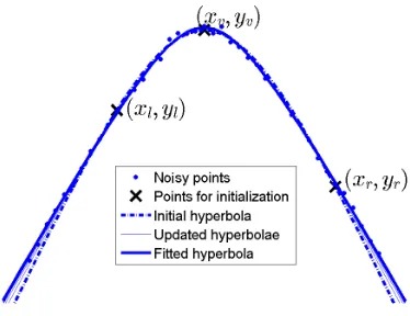
To facilitate the evaluation of the experimental results with the ground truth, we use a simple way to represent hyperbolae in the ground truth. For each hyperbola in the ground truth, three points are marked manually: the apex, one point on the left hand side of the apex, and another point on the right hand side of it (Figure 13). All the coordinates of the marked points are recorded in a text file with respect to different images. For a fitted hyperbola in a certain test image, if a group of three marked points for ground truth are found with average distance to that hyperbola less than 10pixels, this hyperbola is regarded as a true positive otherwise it is taken as a false one.
[image:12.612.349.525.55.198.2]Some experiments on real datasets with the pro-posed method are displayed in Figures 2, 14, and 16. There are 57clusters given by the C3 algorithm in the experiment displayed in Figure 2 and 45
Fig. 13. Example of ground truth in GPR images (Best viewed in colour).
Fig. 14. Some experimental results on real data (Best viewed in colour).
[image:12.612.317.560.267.398.2](a) Results with the unimodal thresholding
[image:13.612.320.558.64.242.2](b) Results with the proposed thresholding
Fig. 15. Comparison of different thresholding methods on one real GPR image: blue curves are the fitted hyperbolae, green rectangles are the correctly found hyperbolae, red rectangles are the hyperbolae missed by the detection algorithm (Best viewed in colour).
C. Comparison of Hyperbola Detection and Fitting Rates with Another Method
We also compared the proposed method with the one introduced in [9]. In [9], a Viola-Jones based detector is used to detect the candidate hyperbola regions at first, and then a generalized Hough trans-form is used to extract hyperbola parameters by fitting hyperbolic edges of each candidate region. As it did not provide any details of the Hough transform based hyperbola fitting results, we compare this method with our proposed method using two met-rics: the detection rate and fitting rate. As mentioned above, if a group of three marked hyperbola points for ground truth are found with average distance
(a) Input image (b) Output im-age
(c) Regions of high response
(d) Some output clusters of the C3 algorithm
Fig. 16. An illustration of the application of the proposed technique on a real GPR image. (a) the input image, (b) output image and (c) the regions of interest. (d) Some clusters obtained from the C3 algorithm (not all clusters from the C3 algorithm are shown here (Best viewed in colour).
to a fitted hyperbola less than 10 pixels, the fitted hyperbola is regarded as a true positive otherwise it is taken as a false one. Since in the proposed method, if a cluster is identified as a hyperbolic signature, a hyperbola is always fitted to that region. So the detection rate and fitting rate of the proposed method are the same. But an obvious difference can be found in the detection rate and fitting rate with the methods proposed in [9].
[image:13.612.75.273.65.235.2]the obtained classifier is used to detect candidate regions in the testing data set. Detailed statistics of the average detection rate of the method used in [9] are given in the first row of Table II. It can be seen that the detection rate is 0.72, but the average precision rate is only 0.35.
TABLE II
COMPARISON OF THE AVERAGE DETECTION RATES AND FITTING RATES AMONG DIFFERENT METHODS
Method Recall Precision F-Measure Detection rates of [9] 0.724 0.347 0.474
Fitting rates of [9] 0.418 0.091 0.149 Fitting rates of [34] + C3 0.638 0.654 0.643 Fitting rate of our method 0.704 0.708 0.702
2) A generalized Hough Transform Based Fitting Rate: As presented in [9], the candidate regions are smoothed with a Gaussian filter to reduce noise and artefacts, and then converted with a Canny edge detector into a binary image. After that, a gener-alized Hough transform is used to fit hyperbolae based on the edge points. For each candidate region, only the best hyperbola given by the generalized Hough transform is fitted. Each fitted hyperbola is then compared with the ground truth with the same criterion as described above. It can be seen in some cases that even a correct region is detected in the detection step the generalized Hough transform fails to fit the correct hyperbola, as shown in Figure 18. The recall rates of the correctly fitted hyperbola from different methods are shown in the second column of Table II and Figure 17. In Figure 17, the two images on the first row are only used to demonstrate the original GPR image overlapped with the detected candidate regions from Viola-Jones based detector, and the figures on the second row are the enlarged windows of the red rectangles in the images on the first row. The top horizontal pattern of the GPR image has no influence on the generalized Hough transform results since each candidate region was then cropped and processed separately for hyperbola fitting.
D. Computational time
[image:14.612.325.549.221.360.2]The size of the synthetic input images is100×100 pixels. The average computational time of the ex-periments on one sample image using a computer with Intel 3.6GHz processor is approximately 0.43 seconds. The computational time on real images
Fig. 17. Comparison of the fitting rates of different methods on 10 cross evaluations.
Fig. 18. The generalized Hough transform fails to fit correct hyperbolae in some detected regions. First row: input GPR images with the ground truth marked by blue rectangles. The red curve is the fitted hyperbola to the region in the red window based on the edge points as shown in the second row. It can be seen the fitted hyperbolae are outside the detected region and are regarded as false fitting (Best viewed in colour).
depend on how many hyperbolae are detected. In our experiments, the sizes of the real input images are 300×400 pixels and the computational time of a real image is on average 0.48 + 0.73×n seconds withnbeing the number of candidate hyperbolae for fitting; on average 6 hyperbolae were detected and fitted in each test image. This speed is fast enough for real time on-site applications.
TABLE III
COMPUTATION TIME OF HYPERBOLA FITTING USING A COMPUTER WITHINTEL3.6GHZ PROCESSOR
Method Fitting time per hyperbola (s)
Generalized Hough transform based fitting method
Discretization values ofds Time
ds= (1,1,1,1) 2.97
ds= (1,1,0.5,0.5) 11.4
ds= (0.5,0.5,0.5,0.5) 47.3
ds= (0.2,0.2,0.2,0.2) 895.3 Proposed hyperbola
fit-ting method
0.73
VI. CONCLUSIONS ANDFUTURE WORK
In this paper a novel technique for automatic in-terpretation of GPR images is introduced. The pro-posed system1 allows for the detection of the
pres-ence of underground buried objects and can obtain hyperbola parameters by fitting a hyperbola to each hyperbolic signature in a completely automatic man-ner. The C3 algorithm is based on the connecting el-ements from adjacent columns of the image which is different from conventional distance/density based clustering techniques. It can not only cluster the separated hyperbolic signatures but also segment intersected or connected hyperbolic signatures into separated ones. The neural network classification al-gorithm for identifying hyperbolic signatures needs only two features and can be trained easily with a small set of training data. The orthogonal distance hyperbola fitting algorithm is robust and efficient for fitting ‘south-opening’ hyperbolae. The hyperbola parameters obtained through the orthogonal distance fitting algorithm can be used in further applications such as estimating the size of the objects [12]. Despite the intrinsic complexity of GPR images, the experimental results show that the proposed method exhibits very good performance compared with a state of the art method, in terms of robustness to noise, efficiency and accuracy and is fast enough for real time on-site applications. The proposed thresholding method works very well compared with other classic thresholding methods, but we believe a “multi-level thresholding” method which we are currently studying may improve the current method even further by adaptively segmenting the weak reflections such as those from small plastic pipes.
1
The code will be placed in an open source repository.
ACKNOWLEDGEMENTS
The financial assistance of the EPSRC under grants EP/F06585X/1 and EP/K021699/1, and the EU under Grant Agreement 280712 is gratefully acknowledged.
REFERENCES
[1] D. Daniels,Ground penetrating radar. London, U. K.: The Inst. Elect. Eng. (IEE), 2004.
[2] C. Bruschini, B. Gros, F. Guerne, P. Y. Pi`ece, and O. Carmona, “Ground penetrating radar and imaging metal detector for antipersonnel mine detection,”Journal of Applied Geophysics, vol. 40, no. 1-3, pp. 59–71, 1998.
[3] G. Ciochetto, S. Delbo, P. Gamba, and D. Roccato, “Fuzzy shell clusering and pipe detection in ground penetrating radar data,”
IGARSS’99, vol. 5, pp. 2575–2577, 1999.
[4] E. Costamagna, P. Gamba, and E. Lossani, “A neural network approach to the interpretation of ground penetrating radar,”
IGARSS’98, vol. 1, pp. 412–414, 1998.
[5] P. Gamba and S. Lossani, “Neural detection of pipe signatures in ground penetrating radar images,” IEEE Transactions on Geoscience and Remote Sensing, vol. 38, pp. 790–797, 2000. [6] R. Janning, T. Horvath, A. Busche, and L. Schmidt-Thieme,
“Gamrec a clustering method using geometrical background knowledge for GPR data preprocessing,” Artificial Intelligence Applications and Innovations (IFIP Advances in Information and Communication Technology 381), pp. 347 – 356, 2012. [7] R. Janning, A. Busche, T. Horvath, and L. Schmidt-Thieme,
“Buried pipe localization using an iterative geometric clustering on GPR data,” Artifical Inteligence Review, vol. 42, pp. 403– 425, 2013.
[8] R. Janning, T. Horvath, A. Busche, and L. Schmidt-Thieme, “Pipe localizationg by apex detection,”Proceedings of the IET international conference on radar systems, pp. 1 – 6, 2012. [9] C. Maas and J. Schmalzl, “Using pattern recognition to
au-tomatically localize reflection hyperbolas in data from ground penetrating radar,” vol. 58, pp. 116–125, 2013.
[10] L. Mertens, R. Persico, L. Matera, and S. Lambot, “Automated detection of reflection hyperbolas in complex GPR images with no a priori knowledge on the medium,”IEEE Transactions on Geoscience and Remote Sensing, vol. 54, no. 1, pp. 580–596, 2016.
[11] E. Pasolli, F. Melgani, and M. Donelli, “Automatic analysis of GPR Images: a pattern-recognition approach,” IEEE Transac-tions on Geoscience and Remote Sensing, vol. 47, no. 7, pp. 2206–2217, 2009.
[12] S. Shihab and W. Al-Nuaimy, “Radius estimation for cylintrical objects detected by ground penetrating radar,” Sensing and Imaging: An International Journal, vol. 6(2), pp. 151–166, 2005.
[13] J. Illingworth and J. Kittler, “A survey of the hough transform,”
Computer vision, graphics, and image processing, vol. 44, no. 1, pp. 87–116, 1988.
[14] L. Capineri, P. Grande, and J. A. G. Temple, “Advanced image-processing technique for real-time interpretation of ground-penetrating radar images,” International Journal of Imaging Systems and Technology, vol. 9, no. 1, pp. 51–59, 1998. [15] P. Falorni, L. Capineri, L. Masotti, and G. Penilli, “3-d radar
[16] C. G. Windsor, L. Capineri, and P. Falorni, “A data pair-labeled generalized Hough transform for radar location of buried objects,”IEEE Geoscience and Remote Sensing Letters, vol. 11, no. 1, pp. 124–127, Jan 2014.
[17] M. Fritze, “Detection of buried landmines using ground pene-trating radar,”SPIE proceedings, vol. 2496, pp. 100–108, 1995. [18] W. Alnuaimy, Y. Huang, M. Nakhkash, M. Fang, V. Nguyen, and A. Erisken, “Automatic detection of buried utilities and solid objects with GPR using neural networks and pattern recognition,”Journal of Applied Geographics, vol. 43, pp. 157– 165, 2000.
[19] P. Viola and M. J. Jones, “Robust real-time face detection,”
International Journal of Computer Vision, vol. 57, no. 2, pp. 137–154, 2004.
[20] A. Giannopoulos, “Modelling ground penetrating radar by gprMax,”Construction and Building Materials, vol. 19, no. 10, pp. 755–762, 2005.
[21] H. Chen and A. G. Cohn, “Probabilistic robust hyperbola mixture model for interpreting ground penetrating radar data,” inIEEE World Congress on Computational Intelligence, 2010, pp. 3367–3374.
[22] T. Kanungo, D. M. Mount, N. S. Netanyahu, C. D. Piatko, R. Silverman, and A. Y. Wu, “An efficient k-means clustering algorithm: analysis and implementation,”IEEE Trans. Pattern Analysis and Machine Intelligence, vol. 24, pp. 881–892, 2002. [23] R. Ng and J. Han, “Efficient and effective clustering methods for spatial data mining,”Proc. 20th Int. Conf. on Very Large Data Bases, pp. 144–155, 1994.
[24] M. Ester, H.-P. Kriegel, J. Sander, and X. Xu, “A density-based algorithm for discovering clusters in large spatial databases with noise,” The Second International Conference on Knowledge Discovery and Data Mining (KDD-96), pp. 226–231, 1996. [25] L. Ert¨oz, M. Steinbach, and V. Kumar, “Finding clusters of
different sizes, shapes, and densities in noisy, high dimensional data,”In Proceedings of Second SIAM International Conference on Data Mining, 2003.
[26] S. Ahn, W. Rauh, and H.-J. Warnecke, “Least-squares orthog-onal distance fitting of circle, sphere, ellipse, hyperbola and parabola,”Pattern Recognition, vol. 34, pp. 2283–2303, 2001. [27] F. L. Booktein, “Fitting conic sections to scattered data,”
Computer Graphics and Image Processing, vol. 9(1), pp. 56– 71, 1979.
[28] A. Fitzgibbon, M. Pilu, and R. B. Fisher, “Direct least square fitting of ellipses,”IEEE Transactions on Pattern Analysis and Machine Intelligence, vol. 21(5), pp. 476–480, 1999.
[29] W. Gander, G. Golub, and R. Strebel, “Least-squares fitting of circles and ellipses,”BIT, vol. 34, pp. 558–578, 1994. [30] M. Pilu, A. Fitzgibbon, and R. B. Fisher, “Ellipse-specific direct
least-square fitting,”In Proceedings of International Conference on Image Processing, vol. 3, 1996.
[31] H. Chen and A. G. Cohn, “Probabilistic conic mixture model and its applications to mining spatial ground penetrating radar data,” in Workshops in SIAM Conference on Data Mining (SDM10), 2010.
[32] N. Otsu, “A Threshold Selection Method from Gray-level His-tograms,”IEEE Transactions on Systems, Man and Cybernetics, vol. 9, no. 1, pp. 62–66, 1979.
[33] J. Kapur, P. Sahoo, and A. Wong, “A new method for gray-level picture thresholding using the entropy of the histogram,”
Computer Vision, Graphics, and Image Processing, vol. 29, no. 3, pp. 273 – 285, 1985.
[34] P. L. Rosin, “Unimodal thresholding,”Pattern Recognition, pp. 2083–2096, 2001.
[35] J. M. Zurada,Introduction to Artificial Neural Systems. USA: West Publishing, 1992.
Qingxu Dou Dr Qingxu Dou is currently a research fellow in the School of Computing at University of Leeds, UK. He obtained his MSc in Applied Mathematics from Heriot-Watt University in 2006, a PhD in Electric and Electronic Engineering from Heriot-Watt Uni-versity in 2011. His research areas of interest are computer vision, sensor data interpretation, data fusion, buried utilities mapping and math-ematical modelling.
Lijun WeiDr Lijun Wei is a research fellow in Computer Science at the University of Leeds, UK. She obtained BSc degree from Wuhan University in China, and a PhD from Univer-sity of Technology of Belfort and Montb´eliard, France. Her main areas of interest are image processing and multi-sensor fusion especially on mapping and intelligent vehicle localiza-tion/navigation.
Derek R. Magee Dr Derek Magee is a lec-turer in Computer Science at the University of Leeds, UK. He obtained a first class BSc Engineering degree from Durham University in 1995, and a PhD from the University of Leeds in 2001. His main areas of interest are image analysis and machine learning in par-ticular applied to Medical Image and Remote sensing data. Additionally, he is chief technical officer of Medical Image Analysis company HeteroGenius Ltd.