Fitting Convex Sets to Data: Algorithms and
Applications
Thesis by
Yong Sheng Soh
In Partial Fulfillment of the Requirements for the Degree of
Doctor of Philosophy
CALIFORNIA INSTITUTE OF TECHNOLOGY Pasadena, California
2019
© 2019 Yong Sheng Soh
ACKNOWLEDGEMENTS
My first and foremost thanks go to my advisor Venkat Chandrasekaran. Reflecting back on my time in graduate school, Venkat has been the mentor that I needed, and perhaps at times, more so than the mentor that I necessarily wanted. Thank you for your dedication and hard work at training me to be an independent researcher. Thank you for your faith in me, and for pushing me hard to realize my potential. It was a tremendous privilege to work with you.
I am grateful to committee members Mathieu Desbrun, Babak Hassibi, Andrew Stuart, and Joel Tropp. Outside this thesis, they have been helpful informal mentors and teachers who have changed the way I think and do research. I also wish to thank Adam Wierman for supporting me throughout my time in graduate school, and for fostering an environment at CMS where I could thrive.
A big thank you to my friends at CMS: Ania Baetica, Max Budninsky, Desmond Cai, Utkan Candogan, Thomas Catanach, Niangjun Chen, Lingwen Gan, Ramya Korlakai, Yoke Peng Leong, Riley Murray, Yorie Nakahira, John Pang, and Armeen Taeb. It has been a blessing to learn from you, and be friends with you.
ABSTRACT
This thesis concerns the geometric problem of finding a convex set that best fits a given dataset. Our question serves as an abstraction for data-analytical tasks arising in a range of scientific and engineering applications. We focus on two specific instances:
1. A key challenge that arises in solving inverse problems is ill-posedness due to a lack of measurements. A prominent family of methods for addressing such issues is based on augmenting optimization-based approaches with a convex penalty function so as to induce a desired structure in the solution. These functions are typically chosen using prior knowledge about the data. In Chapter 2, we study the problem of learning convex penalty functions directly from data for settings in which we lack the domain expertise to choose a penalty function. Our solution relies on suitably transforming the problem of learning a penalty function into a fitting task.
2. In Chapter 3, we study the problem of fitting tractably-described convex sets given the optimal value of linear functionals evaluated in different directions.
Our computational procedures for fitting convex sets are based on a broader frame-work in which we search among families of sets that are parameterized as linear projections of a fixed structured convex set. The utility of such a framework is that our procedures reduce to the computation of simple primitives at each iteration, and these primitives can be further performed in parallel. In addition, by choosing structured sets that are non-polyhedral, our framework provides a principled way to search over expressive collections of non-polyhedral descriptions; in particular, con-vex sets that can be described via semidefinite programming provide a rich source of non-polyhedral sets, and such sets feature prominently in this thesis.
We provide performance guarantees for our procedures. Our analyses rely on understanding geometrical aspects of determinantal varieties, building on ideas from empirical processes as well as random matrix theory. We demonstrate the utility of our framework with numerical experiments on synthetic data as well as applications in image denoising and computational geometry.
1. In Chapter 4, we consider the problem of optimally approximating a convex set as a spectrahedron of a given size. Spectrahedra are sets that can be expressed as feasible regions of a semidefinite program.
PUBLISHED CONTENT AND CONTRIBUTIONS
Y. S. Soh and V. Chandrasekaran (2015). “High-Dimensional Change-Point Es-timation: Combining Filtering with Convex Optimization”. In 2015 IEEE Inter-national Symposium on Information Theory (ISIT), Hong Kong, June 2015. DOI
10.1109/ISIT.2015.7282435
Y.S.S participated in the conception of the project, performed the analysis, undertook the numerical experiments, and participated in the writing of the manuscript.
Y. S. Soh and V. Chandrasekaran (2017). “High-Dimensional Change-Point Esti-mation: Combining Filtering with Convex Optimization”. InApplied and Computa-tional Harmonic Analysis43,1, pp 122–147. DOI10.1016/j.acha.2015.11.003 Y.S.S participated in the conception of the project, performed the analysis, undertook the numerical experiments, and participated in the writing of the manuscript.
TABLE OF CONTENTS
Acknowledgements . . . iii
Abstract . . . iv
Published Content and Contributions . . . vi
Table of Contents . . . vii
List of Illustrations . . . ix
List of Tables . . . xiii
Chapter I: Introduction . . . 1
1.1 Notation and Conventions . . . 8
Chapter II: Learning Semidefinite Regularizers . . . 9
2.1 Introduction . . . 9
2.2 An Alternating Update Algorithm for Learning Semidefinite Regu-larizers . . . 18
2.3 Convergence Analysis of Our Algorithm . . . 28
2.4 Numerical Experiments . . . 42
2.5 Discussion . . . 49
Chapter III: Fitting Tractable Convex Sets to Support Function Evaluations . . 54
3.1 Introduction . . . 54
3.2 Projections of Structured Convex Sets . . . 60
3.3 Main Results . . . 65
3.4 Algorithms . . . 85
3.5 Numerical Experiments . . . 88
3.6 Conclusions and Future Directions . . . 94
Chapter IV: Optimal Approximations of Convex Sets as Spectrahedra . . . . 97
4.1 Introduction . . . 97
4.2 Optimal Approximations of Compact Sets as Spectrahedra of Fixed Size . . . 98
4.3 Algorithms . . . 100
4.4 Numerical Experiments . . . 101
Chapter V: High-Dimensional Change-Point Estimation: Combining Filter-ing with Convex Optimization . . . 106
5.1 Introduction . . . 106
5.2 Background on Structured Signal Models . . . 110
5.3 Convex Programming for Change-Point Estimation . . . 113
5.4 Tradeoffs in High-Dimensional Change-Point Estimation . . . 119
5.5 Numerical Results . . . 125
5.6 Conclusions . . . 129
Chapter VI: Conclusions . . . 130
6.1 Summary of Contributions . . . 130
Appendix A: Proofs for Chapter 2 . . . 133
A.1 Proofs of Lemma 2.3.9 and Lemma 2.3.10 . . . 133
A.2 Proof of Proposition 2.3.8 . . . 133
A.3 Stability of Matrix and Operator Scaling . . . 138
A.4 Proof of Proposition 2.3.7 . . . 143
A.5 Proof of Proposition 2.3.1 . . . 145
A.6 Proof of Proposition 2.3.2 . . . 146
A.7 Proof of Proposition 2.3.3 . . . 152
A.8 Proof of Proposition 2.3.4 . . . 153
A.9 Proof of Proposition 2.3.6 . . . 153
Appendix B: Proofs of Chapter 3 . . . 155
Appendix C: Proofs of Chapter 5 . . . 159
C.1 Relationship between Gaussian distance and Gaussian width . . . 159
C.2 Analysis of proximal denoising operators . . . 163
C.3 Proofs of results from Section 5.3 . . . 164
LIST OF ILLUSTRATIONS
Number Page
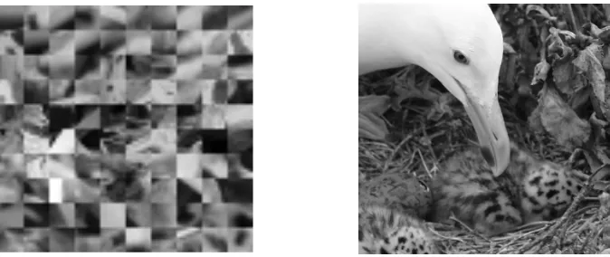
2.1 Average number of iterations required to identify correct regularizer as a function of the number of observations; each line represents a fixed noise level σ denoting the amount of corruption in the initial guess (see Section 2.4.1 for details of the experimental setup). . . 42 2.2 Image patches (left) obtained from larger raw images (sample on the
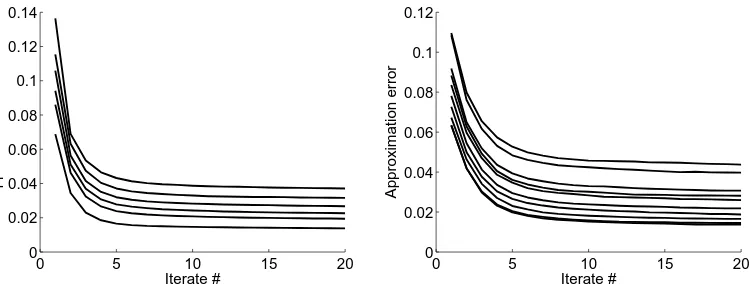
right). . . 44 2.3 Progression in mean-squared error with increasing number of
itera-tions with random initializaitera-tions for learning a semidefinite regular-izer (left) and a polyhedral regularregular-izer (right). . . 46 2.4 Comparison between atoms learned from dictionary learning (left)
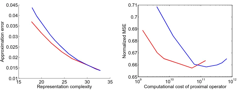
and our algorithm (right). . . 46 2.5 Comparison between dictionary learning (blue) and our approach
(red) in representing natural image patches (left); comparison be-tween polyhedral (blue) and semidefinite (right) regularizers in de-noising natural image patches (right). . . 48 2.6 Progression of our algorithm in recovering regularizers in a synthetic
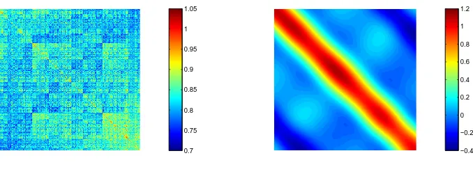
experimental set-up; the horizontal axis represents the number of iterations, and each line corresponds to a different random initial-ization. The left subplot shows a problem instance in which all 10 different random initializations recover a global minimizer, while the right subplot shows a different problem instance in which 4 out of 10 random initializations lead to local minima. . . 51 2.7 Gram matrices of images of sparse vectors (left) and low-rank
matri-ces (right). . . 51 2.8 Dataset of rotated image patches. . . 52 2.9 A collection of six atoms learned from the data using dictionary
learning. . . 52 2.10 A semidefinite representable dictionary learned from the data. . . 53 2.11 Residual error from representing dataset as projections of a rank-one
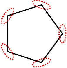
3.2 Estimating a regular 5-gon as the projection of ∆5. In the large n
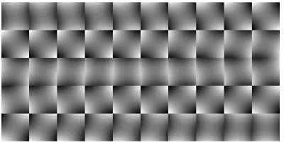
limit, the estimator ˆKn(C)is a 5-gon. The typical deviation of the vertices of ˆKn(C)from that of the 5-gon (scaled by a factor of√n) is represented by the surrounding ellipses. . . 74 3.3 Modes of oscillations for an estimate of the`2-ball inR2. . . 75 3.4 Estimating K?the spectral norm ball in S2 as the projection of the
set C (3.9). The extremal points of the estimator ˆKn(C) comprise
a connected component that is isomorphic to S1 (see the above ac-companying discussion), and the above figure describes the possible modes of oscillations. There are 8 modes altogether – 5 of which occurs in the xy-plane and are described in Figure 3.3, and the re-maining 3 are shown in (b),(c), and (d). . . 76 3.5 Reconstructions of the unit`1-ball (left) inR3from 200 noisy support
function measurements using our method withC =∆6(second from left), and with C = ∆12 (third from left). The LSE is the rightmost figure. . . 80 3.6 Reconstruction of the unit`∞ball inR3from 75 noisy support
func-tion measurements using our method. The choice of lifting set is
C= ∆8. . . 82 3.7 Reconstruction of the Race Track from 200 noisy support function
measurements using our method. The choice of lifting set is the free spectrahedronO4. . . 83 3.8 Reconstruction of the unit`1-ball inR3from noiseless (first row) and
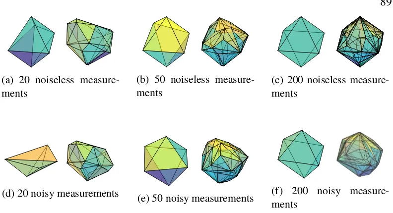
noisy (second row) support function measurements. The reconstruc-tions obtained using our method (with C = ∆6 in (3.2)) are the on the left of every subfigure, while the LSE reconstructions are on the right of every subfigure. . . 89 3.9 Reconstruction of the unit`2-ball inR3from noiseless (first row) and
noisy (second row) support function measurements. The reconstruc-tions obtained using our method (with C = O3 in (3.2)) are the on the left of every subfigure, while the LSE reconstructions are on the right of every subfigure. . . 90 3.10 Approximating the`1-ball inR2as the projection of the free-spectrahedron
inS2(left),S3(center), andS4(right). . . 91 3.11 Approximating the `1-ball inR3as the projection of free
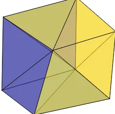
3.12 Reconstructions of K? (defined in (3.16)) as the projection of O3
(top row) and O4 (bottom row). The figures in each row are dif-ferent views of a single reconstruction, and are orientated in the
(0,0,1),(0,1,0),(1,0,1), and(1,1,0)directions (from left to right)
re-spectively. . . 91
3.13 Approximating the `2-ball in R3 as the projection of ∆q for q ∈ {4,5, . . . ,12} (from left to right, top to bottom). . . 93
3.14 Reconstructions of the left lung from 50 support function measure-ments (top row) and 300 support function measuremeasure-ments (bottom row). Subfigures (a),(b),(c),(d),(f),(g),(h), and (i) are projections of free spectrahedra with dimensions as indicated, and subfigures (e) and (j) are LSEs. . . 94
3.15 Choosing the lifting dimension in a data-driven manner. The left sub-plot shows the cross validation error of reconstructing the`1-ball inR3as the projection of∆qover different choices ofq, and the right sub-plot shows the same quantity for KS3 ⊂ R3 (see accompanying text) as the projection ofOpover different choices ofp. . . 96
4.1 {(x,y): x4+y4 ≤ 1}, also known as the TV-screen. . . 102
4.2 Approximations of the TV-screen as spectrahedra. . . 102
4.3 Approximations of the TV-screen as polyhedra. . . 103
4.4 An non-semialgebraic set defined as{(x,y): x ≤ 1/2,y ≤ 1/2,exp(−3/2− x) −1/2≤ y}. . . 104
4.5 Approximations of C2as spectrahedra. . . 104
4.6 Mean Squared Errors of approximations of C2 as spectrahedra of different sizes. . . 104
4.7 Reconstructions of conv(V) using our method. The variety V is outlined in blue. . . 105
4.8 Mean Squared Errors of approximations of conv(V)as spectrahedra . 105 5.1 Experiment contrasting our algorithm (in blue) with the filtered derivative approach (in red): the left sub-plot corresponds to a small-sized change and the right sub-plot corresponds to a large-small-sized change.126 5.2 Plot of estimated points: the locations of the actual change-points are indicated in the bottom row. . . 127
5.4 Experiment from Section 5.5 demonstrating a phase transition in the recovery of the set of change-points for different values of ∆min and
Tmin. The black cells correspond to a probability of recovery of 0 and the white cells to a probability of recovery of 1. . . 129 C.1 Figure showing the`1-norm ballC1with parameterκC1(x1)= 1. . . . 160 C.2 Figure showing the skewed√ `1-norm ballC2with parameterκC2(x2)=
LIST OF TABLES
Number Page
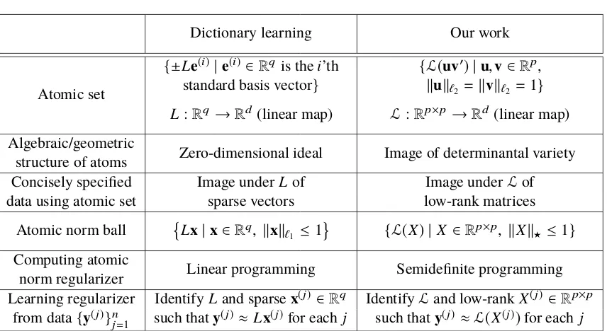
2.1 A comparison between prior work on dictionary learning and the present paper. . . 14 4.1 Mean Squared Errors of approximations of the TV-screen as
polyhe-dra and spectrahepolyhe-dra of different sizes. . . 103 5.1 Table of parameters employed in our change-point estimation
C h a p t e r 1
INTRODUCTION
The heart of this thesis concerns the geometric problem of finding a convex set
C ⊂ Rdthat best fits a given dataset. Recall that a set Cisconvexif it satisfies the following property:
λx+(1−λ)y ∈ Cfor everyx,y ∈ C, and everyλ∈ [0,1].
The task of fitting a convex set to data serves as an abstraction of data-analytical tasks arising in a range of scientific and engineering applications. For example, in econometrics, one may wish to learn a convexity-based model to describe supply-demand levels of a specific commodity based on historical data; here, convexity-based considerations arise naturally as a result of fundamental principles such as marginal utility. In computational geometry, the computation of convex sets to encompass a collection of points in space is a routinely applied procedure, and it serves as a building block for describing more complicated objects.
The nature of the data that is presented here may take many forms; for instance, they may reveal direct information aboutC in the form of points lying on the boundary ofC, or they may reveal indirect information aboutCin the form of optimal values of a collection of functions evaluated overC. The precise manner in which we fit a convex set depends on the type of data we receive as well as the purpose for which we fit these sets. In Chapters 2 and 3, we focus on two specific instances of fitting problems, and we summarize the contributions of these chapters as follows:
penalty function) is informed by domain-specific knowledge about the data; for instance, certain classes of signals are known to be well-approximated as being sparse in the Fourier domain, and a natural choice of regularizer that is effective at inducing such structure is the`1norm with respect to the Fourier basis. Unfortunately, the challenge in many contemporary data-analytical tasks arising in scientific and engineering applications is that the data is fre-quently high-dimensional, and is presented in an unstructured manner. These challenges complicate the task of providing an informed choice of regular-izer. To address these issues, we propose a framework forlearninga suitable regularizer directly from data.
Our first contribution is to provide a conceptual link between the problem of learning a regularizer from data and the task of identifying a suitable atomic set. More precisely, atomic sets are collections of vectors – we refer to these as atoms– that specify a model for representing data succinctly. The relevance of atomic sets to our set-up is that they identify natural choices of regularizers that are effective at enforcing latent structure present in the data.
Our second contribution is to show that the simplest instantiation of learning a regularizer precisely corresponds to the more widely studied problem of ‘dictionary learning’ or ‘sparse coding’ – these concern the task of represent-ing data as linear projections of sparse vectors. As we elaborate further in Chapter 2, the regularizers that we learn from dictionary learning correspond to identifying a finite collection of atoms for data, and are computable via linear programming.
with respect to these varieties), as well as ideas from random matrix theory. Our fourth contribution is to demonstrate the utility of our framework for learning regularizers, and in particular, regularizers that correspond to an infinite collection of atoms. We consider a numerical task in which we denoise a collection of natural images corrupted by noise. Our results show that the denoisers obtained using our framework attain the same performance as denoisers obtained using prior works based on dictionary learning, but are computationally cheaper to evaluate.
2. Chapter 3: Fitting Tractable Convex Sets to Support Function Evalua-tions. In this chapter, we consider the problem of reconstructing a convex set given optimal values of linear functionals evaluated in different directions. More formally, given a vectoru ∈Rd with unit Euclidean-norm, thesupport functionof a convex setC ⊂ Rd evaluated in the directionu ∈Rdis defined ashC(u)=supg∈Chg,ui. Our task is to estimate an unknown compact convex
C? ⊂ Rdgiven access to its support function evaluations, which may further
be corrupted by noise{(u(i),y(i)): y(i) = hC?(u(i))+(i)}.
The task of reconstructing convex sets from their support function measure-ments arises in a range of applications; for instance, in tomographic appli-cations, the extent of the absorption of parallel rays projected onto an object provides support information about the object. Previous approaches for es-timating convex sets from support function measurements typically rely on estimators that minimize the error over all possible compact convex sets. Un-fortunately, the drawback of such approaches is that they do not allow for the incorporation of prior structural information about the underlying set, and the resulting estimates become increasingly more complicated to describe as the number of measurements available grows. In addition, these estimates are fre-quently specified in terms of polyhedral descriptions, and are thus inadequate for expressing non-polyhedral sets.
sets we achieve two outcomes: from a computational viewpoint, one can op-timize linear functionals over estimators that we obtain as outputs from our procedures efficiently, and from an inferential perspective, weregularize for the complexity of the reconstruction.
We provide a geometric characterization of the asymptotic behavior of our estimators. Our analysis relies on a results that shows certain sets which admit semialgebraic descriptions are Vapnik-Chervonenkis (VC) classes. We apply our numerical procedures to a range of reconstruction tasks including computing a convex mesh of the human lung as well as (a variant of) fitting points on the unit-sphere inR3so as to maximize separation. Our numerical experiments highlight the utility of our framework over previous approaches in settings in which the measurements available are noisy or small in number as well as those in which the underlying set to be reconstructed is non-polyhedral.
A Framework for Fitting. At the core of Chapters 2 and 3 is a broader framework for fitting convex sets based on searching over families specified aslinear projections of ‘structured’ convex sets:
C = {A(C): A∈ L(Rq,Rd)}. (1.1) For instance, in Chapter 3, we consider fitting with sets that are expressible as the projection of the simplex – this is the collection of non-negative vectors whose entries sum up to one:
∆q:= {x:x=(x1, . . . ,xq)0,hx,1i= 1,xi ≥ 0,1≤ i ≤ q} ⊂Rq.
In addition, in Chapter 3, we also consider fitting with sets that are expressible as the projection of the free spectrahedron – this is the collection of positive semidef-inite matrices whose eigenvalues sum up to one, and can be viewed as a suitable generalization of the simplex:
Op:= {X : X = X0,trace(X)= hX,Ii= 1, λi(X) ≥ 0,1≤ i ≤ p} ⊂ Sp.
−x ∈ C wheneverx ∈ C. As such, in Chapter 2, we primarily consider projections of the`1ball (also known as the cross-polytope)
(
x:x= (x1, . . . ,xq)0,
Õ
i=1
|xi| ≤1
)
⊂ Rq,
as well as the nuclear-norm ball
(
X :
p Õ
i=1
σi(X) ≤1 )
⊂ Rp×p, σi(·)is thei-th singular value.
The parameterization of families of convex sets as linear images of structured sets in (1.1) is a central idea in optimization as such families offer a powerful and expressive framework for describing feasible regions of convex programs. In the context of fitting convex sets to data, we search over families parameterized as (1.1) for similar reasons, and we elaborate on these as well as additional reasons in the following. First, as noted above, the parameterization of convex sets as linear images of struc-tured sets as in (1.1) offers a very expressive framework for describing convex sets. As a simple example to illustrate our point, every polytope with at mostqvertices can be represented as the linear image of the simplex ∆q ⊂ Rq via an appropriate projection map A∈ L(Rq,Rd).
Second, by choosing structured convex sets that are non-polyhedral, our framework offers a principled approach for searching over collections of non-polyhedral sets. The capacity to accommodate non-polyhedral descriptions within our framework is a significant contribution of this thesis over prior works. As we elaborate in subsequent chapters, these prior works can be viewed suitably as instances of fitting convex sets with polyhedral descriptions to data.
settings, it is crucial that we are able to perform computations such as optimization over our fitted sets efficiently.
Fourth, we have effective computational strategies for searching over convex sets specified in the form of (1.1). The computational task of searching over families described as (1.1) naturally leads to an optimization instance over the space of linear maps L(Rq,Rd). As we elaborate further in Chapters 2 and 3, such a task may be subsequently reformulated in terms of the structured factorization of a data matrix. The utility of such a reformulation is that we have access to a vast literature of prior works on computing matrix factorizations, and this is helpful for developing computational strategies for our fitting task. The procedures we develop in Chapters 2 and 3 are based on the idea that we compute structured factorizations by optimizing over one factor while keeping the other factor fixed. Such methods are frequently termed as ‘alternating minimization’-based approaches, and they heavily rely on the minimization of each factor being relatively simple to compute. In the current context whereby we search over families parameterized by (1.1), the minimization of our associated matrix factorization instance over each factor requires computations that involve the facial structure of C. Consequently, it is advantageous to select choices ofCfor which its facial geometry is well-understood. Examples of sets that satisfy such a property include the simplex, the free spectrahedron, the`1ball, and the nuclear norm ball.
Semidefinite Programming-Representable Convex Sets. A key emphasis of this thesis is that we fit using sets that can be described via semidefinite programming. Such sets are non-polyhedral, and they naturally generalize the collection of sets that can be described via linear programming, i.e., the collection of polyhedral sets. A range of basic but important questions naturally arise in the context of fitting convex sets with semidefinite descriptions. For instance, one may wish to identify settings under which using semidefinite descriptions over polyhedral descriptions is advantageous. Another question is that one may wish to further understand the expressiveness of semidefinite descriptions. We investigate a simplified version of the latter question in Chapter 4, and we summarize the contributions of this chapter as follows:
as optimization. The collection of spectrahedra is widely known to be very expressive; for instance, it includes the collection of all polyhedra. However, unlike the family of polyhedra, our understanding of spectrahedra is far more limited.
In this chapter, we focus on understanding theexpressivenessof spectrahedra as convex sets. More precisely, we pose the following mathematical question: Given a compact convex C ⊂ Rd, what is its optimal approximation as a
spectrahedron of size k (i.e. the spectrahedron can be expressed in terms of a linear matrix inequality with matrices of size k × k)? Building off ideas developed in Chapter 3, we develop numerical procedures for computing such approximations. Our computational tools are useful for understanding the ex-pressiveness of spectrahedral sets from an approximation-theoretic viewpoint. We demonstrate numerical implementations of our procedure; in particular, we describe some examples of convex sets in which spectrahedra of small sizes offer a surprisingly high degree of approximation.
Secondary Contributions. As a secondary contribution, in Chapter 5, we consider the problem of estimating changes in a sequence of high-dimensional signals given noisy observations. We outline the contributions of Chapter 5 as follows:
guarantees for reliable change-point estimation that require the underlying signal to remain unchanged for long portions of the sequence.
In this chapter, we propose a new approach for estimating change-points in high-dimensional signals by integrating ideas fromatomic norm regulariza-tionwith the filtered derivative framework. The atomic norm regularization step is based on solving a convex optimization instance, and it exploits latent low-dimensional structure that is frequently found in signals encountered in practice. The specific choice of regularization may be selected based on prior knowledge about the data, or it may be learned from data using the ideas from Chapter 2. Our algorithm is well-suited to the high-dimensional setting both in terms of computational scalability and of statistical efficiency. More precisely, our main result shows that our method performs change-point esti-mation reliably as long as the product of the smallest-sized change (measured in terms of the Euclidean-norm-squared of the difference between signals at a change-point) and the smallest distance between change-points (as the number of time instances) are larger than a Gaussian width parameter that character-izes the low-dimensional complexity of the underlying signal sequence. Last, our method is applicable in online settings as it operates on small portions of the sequence of observations at a time.
1.1 Notation and Conventions
The styles of all variables and quantities follow these rules: a is a scalar, a is a vector, Ais a matrix, andAis a linear operator mapping matrices to matrices. Ais typically a set, whileA is acollection. Adenotes a linear map from the space of matrices to vectors.
We use d to refer to the ambient dimension, and we use q to refer to the lifted dimension. The exception is when we lift to the space of matrices, in which case we denote usingp×pdimensions. We typically usesto denote the number of nonzero entries of a vector, i.e.,sparsity, andr to denoterankof a matrix.
C h a p t e r 2
LEARNING SEMIDEFINITE REGULARIZERS
2.1 Introduction
Regularization techniques are widely employed in the solution of inverse problems in data analysis and scientific computing due to their effectiveness in addressing difficulties due to ill-posedness. In their most common manifestation, these methods take the form of penalty functions added to the objective in optimization-based approaches for solving inverse problems. The purpose of the penalty function is to induce a desired structure in the solution, and these functions are specified based on prior domain-specific expertise. For example, regularization is useful for promoting smoothness, sparsity, low energy, and large entropy in solutions to inverse problems in image analysis, statistical model selection, and the geosciences [26, 30, 32, 35, 36, 48, 99, 116, 144]. In this paper, we study the question of learning suitable regularization functions from data in settings in which precise domain knowledge is not directly available. The regularizers obtained using our framework are specified as convex functions that can be computed efficiently via semidefinite programming, and therefore they can be employed in tractable convex optimization approaches for solving inverse problems.
We begin our discussion by highlighting the geometric aspects of regularizers that make them effective in promoting a desired structure. In particular, we focus on a family of convex regularizers that is useful for inducing a general form of sparsity in solutions to inverse problems. Sparse data descriptions provide a powerful formalism for specifying low-dimensional structure in high-dimensional data, and they feature prominently in a range of problem domains. For example, natural images are often well-approximated by a small number of wavelet coefficients, financial time series may be characterized by low-complexity factor models, and a small number of genetic markers may constitute a signature for disease. Concretely, supposeA ⊂ Rdis a (possibly infinite) collection of elementary building blocks or
atoms. Theny ∈Rd is said to have a sparse representation using the atomic setA
ifycan be expressed as follows:
y=
k Õ
i=1
for a relatively small number k. As an illustration, if A = {±e(j)}d
j=1 ⊂ R
d
is the collection of signed standard basis vectors in Rd, then concisely described objects with these atoms are those vectors in Rd consisting of a small number of nonzero coordinates. Similarly, if A is the set of rank-one matrices, then the corresponding sparsely represented entities are low-rank matrices; see [35] for a more exhaustive collection of examples. An important virtue of sparse descriptions based on an atomic set A is that employing the atomic norm induced by A — the gauge function of the atomic set A — as a regularizer in inverse problems offers a natural convex optimization approach for obtaining solutions that have a sparse representation using A [35]. Continuing with the examples of vectors with few nonzero coordinates and of low-rank matrices, regularization with the `1 norm (the gauge function of the signed standard basis vectors) and with the matrix nuclear norm (the gauge function of the unit-Euclidean-norm rank-one matrices) are prominent techniques for promoting the corresponding sparse descriptions in solutions to inverse problems [30, 32, 36, 48, 53, 99, 116, 144]. The reason for the effectiveness of atomic norm regularization is the favorable facial structure of the convex hull of A, which has the feature that all its low-dimensional faces contain points that have a sparse description usingA. Indeed, in many contemporary data analysis applications the solutions of regularized optimization problems with generic input data tend to lie on low-dimensional faces of sublevel sets of the regularizer [31, 48, 116]. Based on this insight, atomic norm regularization has been shown to be effective in a range of tasks such as statistical denoising, model selection, and system identification [20, 107, 127].
The difficulty with employing an atomic norm regularizer in practice is that one requires prior domain knowledge of the atomic set A – the extreme points of the atomic norm ball – that underlies a sparse description of the desired solution in an inverse problem. While such information may be available based on domain exper-tise in some problems (e.g., certain classes of signals having a sparse representation in a Fourier basis), identifying a suitable atomic set is challenging for many contem-porary data sets that are high-dimensional and are typically presented to an analyst in an unstructured fashion. In this paper, we study the question of learning a suitable regularizer directly from observations {y(j)}nj=
1 ⊂ R
d of a collection of structured
that eachy(j) has a sparse representation usingA; the corresponding regularizer is simply the atomic norm induced byA. A norm with these characteristics is adapted to the structure contained in the data{y(j)}nj=
1, and it can be used subsequently as a regularizer in inverse problems to promote solutions with the same type of structure as in the collection{y(j)}nj=
1.
When considered in full generality, our question is somewhat ill-posed for several reasons. First, if k · k is a norm that satisfies the properties described above with respect to the data{y(j)}n
j=1, then so doesαk · kfor any positive scalarα. This issue is addressed by learning a norm from a suitably scaled class of regularizers. A second source of difficulty is that the Euclidean normk·k`2trivially satisfies our requirements for a regularizer as eachy(j)/ky(j)k`2is an extreme point of the Euclidean norm ball in Rd; indeed, this is the regularizer employed in ridge regression. The atomic set in this case is the collection of all points with Euclidean norm equal to one, i.e., the dimension of this set is d −1. However, data sets in many applications throughout science and engineering are well-approximated as sparse combinations of elements of atomic sets of much smaller dimension [12, 26, 35, 45, 83, 104, 111]. Identifying such lower-dimensional atomic sets is critical in inverse problems arising in high-dimensional data analysis in order to address the curse of dimensionality; in particular, as discussed in some of these preceding references, the benefits of atomic norm regularization in problems with large ambient dimension d are a consequence of measure concentration phenomena that crucially rely on the small dimensionality of the associated atomic set in comparison to d. We circumvent this second difficulty in learning a regularizer by considering atomic sets with appropriately bounded dimension. A third challenge with our question as it is stated is that the gauge function of the set{±y(j)/ky(j)k`2}
n
j=1also satisfies the requirements for a suitable atomic norm as eachy(j)/ky(j)k`2 is an extreme point of the unit ball of this regularizer. However, such a regularizer suffers from overfitting and does not generalize well as it is excessively tuned to the data set{y(j)}n
j=1. Further, for large n this gauge function becomes intractable to characterize, and it does not offer a computationally efficient approach for regularization. We overcome this complication by considering regularizers that have effectively parametrized sets of extreme points, and consequently are tractable to compute.
The problem of learning a suitable polyhedral regularizer – an atomic norm with a unit ball that is a polytope – from data points {y(j)}n
equivalent to the question of ‘dictionary learning’ (also called ‘sparse coding’) on which there is a substantial amount of prior work [2–4, 8, 9, 11, 72, 104, 122, 123, 134, 139, 140, 148] (see also the survey articles in [51, 96]). To see this connection, suppose without loss of generality that we parametrize a finite atomic set via a matrixL ∈Rd×qso that the columns ofLand their negations specify the atoms. The associated atomic norm ball is the image underL of the`1ball inRq. The columns of L are typically scaled to have unit Euclidean norm to address the scaling issues mentioned previously (see Section 2.2.4). The number of columns q controls the complexity of the atomic set as well as the computational tractability of describing the atomic norm, and is permitted to be larger than d (i.e., the ‘overcomplete’ regime). With this parametrization, learning a polyhedral regularizer to promote the type of structure contained in{y(j)}nj=
1may be viewed as obtaining a matrixL(given a target number of columnsq) such that eachy(j) is well-approximated asLx(j) for a vectorx(j) ∈ Rqwith few nonzero coordinates. Computing such a representation of the data is precisely the objective in dictionary learning, although this problem is typically not phrased as a quest for a polyhedral regularizer in the literature. We remark further on some recent algorithmic developments in dictionary learning in Sections 2.1.3.1 and 2.2.4, and we contrast these with the methods proposed in the present paper.
2.1.1 From Polyhedral to Semidefinite Regularizers
concerns by considering atomic sets that are efficiently parametrized as algebraic varieties (of a particular form), and that have convex hulls with tractable semidefinite descriptions. Thus, previous efforts in the dictionary learning literature on identify-ing finite atomic sets may be viewed as learnidentify-ing zero-dimensional ideals, whereas our approach corresponds to learning atomic sets that are larger-dimensional vari-eties. From a computational viewpoint, dictionary learning provides atomic norm regularizers that are computed via linear programming, while our framework leads to semidefinite programming regularizers. Consequently, although our framework is based on a much richer family of atomic sets in comparison with the finite sets considered in dictionary learning, we still retain efficiency of parametrization and computational tractability based on semidefinite representability.
Formally, we consider atomic sets inRdthat are images of rank-one matrices:
Ap(L)= L(uv0) |u,v∈Rp, kuk`2 = 1,kvk`2 = 1 , (2.1) whereL : Rp×p → Rd specifies a linear map. We focus on settings in which the dimensionpis such thatp2> d, so the atomic setsAp(L)that we study in this paper are projections of rank-one matrices from a larger-dimensional space (in analogy to the overcomplete regime in dictionary learning). By construction, elements of Rd that have a sparse representation using the atomic set Ap(L)are those that can be specified as the image under Lof low-rank matricesin Rp×p. As the convex hull of unit-Euclidean-norm rank-one matrices inRp×pis the nuclear norm ball inRp×p, the corresponding atomic norm ball is given by:
conv Ap(L) =
L(X) | X ∈Rp×p, kXk? ≤ 1 , (2.2) where kXk? := Í
iσi(X). As the nuclear norm ball has a tractable semidefinite
description [53, 116], the atomic norm induced byAp(L)can be computed efficiently using semidefinite programming.
Given a collection of data points{y(j)}nj=
1 ⊂ R
dand a target dimension
p, our goal is to find a linear map L : Rp×p → Rd such that each y(j), upon normalization by the gauge function of Ap(L), lies on a low-dimensional face of conv(Ap(L)). For each y(j) to have this property, it must have a sparse representation using the atomic set Ap(L); that is, there must exist a low-rank matrix X(j) ∈ Rp×p
with y(j) = L(X(j)). The matrix X(j) provides a concise description of y(j) ∈ Rd
Dictionary learning Our work
Atomic set
{±Le(i) |e(i) ∈Rq is thei’th {L(uv0) |
u,v∈Rp,
standard basis vector} kuk`2 =kvk`2 =1}
L:Rq →Rd(linear map) L:Rp×p →Rd(linear map)
Algebraic/geometric
Zero-dimensional ideal Image of determinantal variety structure of atoms
Concisely specified Image underLof Image underLof data using atomic set sparse vectors low-rank matrices
Atomic norm ball Lx|x∈Rq, kxk`1 ≤ 1 {L(X) | X ∈R
p×p, kXk
?≤1}
Computing atomic
Linear programming Semidefinite programming norm regularizer
Learning regularizer IdentifyLand sparsex(j)∈Rq IdentifyLand low-rankX(j) ∈
Rp×p
[image:27.612.110.538.62.296.2]from data{y(j)}nj=1 such thaty(j)≈ Lx(j)for each j such thaty(j)≈L(X(j))for each j
Table 2.1: A comparison between prior work on dictionary learning and the present paper.
nuclear norm ball may be phrased as one ofmatrix factorization. In particular, let
Y =[y(1)| · · · |y(n)] ∈Rd×ndenote the data matrix, and letLi ∈Rp×p, i= 1, . . . ,dbe the matrix that specifies the linear functional corresponding to thei’th component of a linear mapL:Rp×p →Rd. Then our objective can be viewed as one of finding a collection of matrices {Li}d
i=1 ⊂ R
p×p specifying linear functionals and a set of
low-rank matrices{X(j)}n j=1 ⊂ R
p×pspecifying concise descriptions such that: Yi,j = hLi,X(j)i i= 1, . . . ,d, j = 1, . . . ,n. (2.3)
Here hA,Bi = tr(A0B) denotes the trace inner product between matrices. Note the distinction with dictionary learning in which one seeks a factorization of the data matrix Y such that the X(j)’s are sparse vectors as opposed to low-rank matrices as in our approach. Figure 2.1 summarizes the key differences between dictionary learning and the present paper.
2.1.2 An Alternating Update Algorithm for Matrix Factorization
A challenge with identifying a semidefinite regularizer by factoring a given data matrix as in (2.3) is that such a factorization is not unique. Specifically, consider any linear map M : Rp×p → Rp×p that is a rank-preserver, i.e., rank(M(X)) = rank(X) for all X ∈ Rp×p; examples of rank-preservers include operators that act
via conjugation by non-singular matrices and the transpose operation. If each y(j) = L(X(j))for a linear mapLand low-rank matrices{X(j)}nj=
that each y(j) = L◦M−1(M(X(j))), where by construction each X(j) has the same rank as the correspondingM(X(j)). This non-uniqueness presents a difficulty as the image of the nuclear norm ball under a linear mapLis, in general, different than it is underL◦M−1for an arbitrary rank-preserverM. Consequently, due to its invariances the factorization (2.3) does not uniquely specify a regularizer. We investigate this point in Section 2.2.2 by analyzing the structure of rank-preserving linear maps, and we describe an approach to associate a unique regularizer to a family of linear maps obtained from equivalent factorizations. Our method entails putting linear maps in an appropriate ‘canonical’ form using the Operator Sinkhorn iterative procedure, which was developed by Gurvits to solve certain quantum matching problems [75]; this algorithm is an operator analog of the diagonal congruence scaling technique for nonnegative matrices developed by Sinkhorn [132].
In Section 2.2 we describe an alternating update algorithm to compute a factorization of the form (2.3). With the Li’s fixed, updating the X(j)’s entails the solution of
affine rank minimization problems. Although this problem is intractable in general [102], in recent years several tractable heuristics have been developed and proven to succeed under suitable conditions [65, 82, 116]. With the X(j)’s fixed, theLi’s
are updated by solving a least-squares problem followed by an application of the Operator Sinkhorn iterative procedure to put the map L in a canonical form as described above. Our alternating update approach is a generalization of methods that are widely employed in dictionary learning for identifying finite atomic sets (see Section 2.2.4).
Section 2.3 contains the main theorem of this paper on the local linear convergence of our alternating update algorithm. Specifically, suppose a collection of data points
{y(j)}n
j=1 ⊂ R
d is generated as y(j) = L?(
X(j)?), j = 1, . . . ,n for a linear map
L? :
Rp×p → Rd that is nearly isometric restricted to low-rank matrices (formally,
L?satisfies arestricted isometry property[116]) and a collection{X(j)?}n j=1 ⊂ R
p×p
of low-rank matrices that is isotropic in a well-defined sense. Given the data{y(j)}nj=
1 as input, our alternating update approach is locally linearly convergent to a linear map
ˆ
L : Rp×p → Rd with the property that the image of the nuclear norm ball inRp×p under ˆLis equal to its image underL?, i.e., our procedure identifies the appropriate regularizer that promotes the type of structure contained in the data {y(j)}nj=
We demonstrate the utility of our framework with a series of experimental results on synthetic as well as real data in Section 2.4.
2.1.3 Related Work
2.1.3.1 Dictionary Learning
As outlined above, our approach for learning a regularizer from data may be viewed as a semidefinite programming generalization of dictionary learning. The alternating update algorithm we propose in Section 2.2.3 for computing a factorization (2.3) gen-eralizes similar methods previously developed for dictionary learning [2, 4, 9, 104] (see Section 2.2.4), and the local convergence analysis of our algorithm in Section 2.3 also builds on previous analyses for dictionary learning [2, 9]. In contrast to these previous results, the development and the analysis of our method in the present paper are more challenging due to the invariances and associated identifiability is-sues underlying the factorization (2.3), which necessitate the incorporation of the Operator Sinkhorn scaling procedure in our algorithm.
Section 2.5.
2.1.3.2 Lifts of Convex Sets
A second body of work with which our paper is conceptually related is the literature on lift-and-project representations (or extended formulations) of convex sets. A tractable lift-and-project representation refers to a description of a ‘complicated’ convex set inRd as the projection of a more concisely specified convex set inRd
0
, with the lifted dimensiond0not being too much larger than the original dimension
d. As discussed in [70, 152], obtaining a suitably structured factorization – of a different nature than that considered in the present paper – of the slack matrix of a polytope (and more generally, of the slack operator of a convex set) corresponds to identifying an efficient lift-and-project description of the polytope. On the other hand, we seek a structured factorization of a data matrix to identify a convex set (i.e., the unit ball of a regularizer) with an efficient extended formulation and with the additional requirement that the data points (upon suitable scaling) lie on low-dimensional faces of the set. This latter stipulation arises in our context from data analysis considerations, and it is a distinction between our setup and the optimization literature on extended formulations.
2.1.3.3 Sinkhorn Scaling
2.1.4 Paper Outline
In Section 2.2 we discuss our alternating update algorithm for computing the fac-torization (2.3) based on an analysis of the invariances arising in (2.3). Section 2.3 gives the main theoretical result concerning the local linear convergence of the algo-rithm described in Section 2.2, and Section 2.4 describes numerical results obtained using our algorithm. We conclude with a discussion of further research directions in Section 2.5.
Notation We denote the Euclidean norm by k · k`2. We denote the operator or spectral norm by k · k2. The k’th largest singular value of a linear map is denoted by σk(·), and the largest and smallest eigenvalues of a self-adjoint linear map are
denoted byλmax(·)andλmin(·)respectively. The space of p×psymmetric matrices is denotedSpand the set of p× psymmetric positive-definite matrices is denoted S++p . The projection map onto a subspace V is denoted PV. The restriction of
a linear map M to a subspace V is denoted by MV. Given a self-adjoint linear
map M : V → V with V being a subspace of a vector space ¯V, we denote the extension of M to ¯V by [M]V¯ : ¯V → V¯; the component in V of the image of any x ∈ V¯ under this map is MPV(x), while the component in V⊥ is the origin.
Given a vector space V, we denote the set of linear operators from V to V by End(V). Given matrices A,B ∈ Rp×p, the linear map A B ∈ End(Rp×p) is specified as A B : X → hB,XiA. The Kronecker product between two linear maps is specified using the standard⊗notation. For a collection of matricesX :=
{X(j)}nj=
1 ⊂ R
p×p, the covariance is specified as cov(X)= 1
n Ín
j=1X
(j)
X(j). Two quantities associated to this covariance that play a role in our analysis areΛ(X) =
1
2(λmax(cov(X))+λmin(cov(X)))and∆(X)= 1
2(λmax(cov(X)) −λmin(cov(X))). Given a matrix X ∈ Rp×p of rank r, the tangent space at X with respect to the
algebraic variety ofp×pmatrices of rank at mostr is specified as1:
T (X)= {X A+BX | A,B ∈Rp×p}.
2.2 An Alternating Update Algorithm for Learning Semidefinite Regularizers In this section we describe an alternating update algorithm to factor a given data matrixY = [y(1)| · · · |y(n)] ∈ Rd×nas in (2.3). As discussed previously, the difficulty with obtaining a semidefinite regularizer using a factorization (2.3) is the existence of infinitely many equivalent factorizations due to the invariances underlying (2.3).
1A rank-r matrixX ∈
Rp×p is a smooth point with respect to the variety ofp×pmatrices of
We begin by investigating and addressing this issue in Sections 2.2.1 and 2.2.2, and then we discuss our algorithm to obtain a regularizer in Section 2.2.3. We contrast our method with techniques that have previously been developed in the context of dictionary learning in Section 2.2.4.
2.2.1 Identifiability Issues
Building on the discussion in the introduction, for a linear map L : Rp×p → Rd
obtained from the factorization (2.3) and for any linear rank-preserverM :Rp×p →
Rp×p, there exists an equivalent factorization in which the linear map isL◦M(note thatM−1is also a rank-preserver ifMis a rank-preserver). As the image of the nuclear norm ball in Rp×p is not invariant under an arbitrary rank-preserver, a regularizer cannot be obtained uniquely from a factorization due to the existence of equivalent factorizations that lead to non-equivalent regularizers. To address this difficulty, we describe an approach to associate a uniqueregularizer to a family of linear maps obtained from equivalent factorizations. We begin by analyzing the structure of rank-preserving linear maps based on the following result [98]:
Theorem 2.2.1 ([98, Theorem 1],[147, Theorem 9.6.2]) An invertible linear op-erator M : Rp×p → Rp×p is a rank-preserver if and only if M is of one of the following two forms for non-singular matricesW1,W2 ∈Rp×p: M(X) =W1XW2or
M(X)=W1X0W2.
This theorem brings the preceding discussion into sharper focus, namely, that the lack of identifiability boils down to the fact that the nuclear norm is not invariant under conjugation of its argument by arbitrary non-singular matrices. However, we note that the nuclear norm ball is invariant under the transpose operation and under conjugation by orthogonal matrices. This observation leads naturally to the idea of employing thepolar decompositionto describe a rank-preserver:
Corollary 2.2.2 Every rank-preserverM : Rp×p → Rp×p can be uniquely decom-posed asM= Mor◦Mpd for rank-preserversMpd :Rp×p→ Rp×pandMor:Rp×p → Rp×pwith the following properties:
• The operatorMoris of one of the following two forms for orthogonal matrices
U1,U2∈Rp×p: Mor(X)=U1XU2orMor(X)=U1X0U2.
Proof. The result follows by combining Theorem 2.2.1 with the polar
decomposi-tion.
We refer to rank-preservers of the type Mpd in this corollary as positive-definite rank-preservers and to those of the typeMor asorthogonal rank-preservers. This corollary highlights the point that the key source of difficulty in identifying a reg-ularizer uniquely from a factorization is due to positive-definite rank-preservers. A natural approach to address this challenge is to put a given linear map L into a ‘canonical’ form that removes the ambiguity due to positive-definite rank-preservers. In other words, we seek a distinguished subset of normalized lin-ear maps with the following properties: (a) for a linear map L, the set {L ◦
Mpd : Mpd is a positive-definite rank-preserver} intersects the collection of nor-malized maps at precisely one point; and (b) for any normalized linear map L, every element of the set {L◦Mor : Mor is an orthogonal rank-preserver} is also normalized. The following definition possesses both of these attributes:
Definition 2.2.3 LetL:Rp×p→ Rdbe a linear map, and letLi ∈Rp×p,i =1, . . . ,d be the component linear functionals of L. Then L is said to be normalized if
Íd
i=1LiLi0= pIandÍdi=1Li0Li = pI.
The utility of this definition in resolving our identifiability issue is based on a paper by Gurvits [75]. Specifically, for a generic linear map L : Rp×p → Rd, the results in [75] imply that there exists auniquepositive-definite rank-preserver
of degree at least two. Consequently, our definition of normalization is in some sense also as ‘simple’ as possible from an algebraic perspective.2
In addition to satisfying these appealing properties, our notion of normalization also possesses an important computational attribute – given a (generic) linear map, a normalizing positive-definite rank-preserver for the map can be computed using the Operator Sinkhorn iterative procedure developed in [75]. Thus, the follow-ing method offers a natural approach for uniquely associatfollow-ing a regularizer to an equivalence class of factorizations.
Obtaining a regularizer from a linear map: Given a linear map L : Rp×p → Rd
obtained from a factorization (2.3), the unit ball of the regularizer we associate to this factorization is the image of the nuclear norm ball inRp×punder the linear map
L◦NL; hereNLis the unique positive-definite rank-preserver that normalizesL(as discussed in the sequel in Corollary 2.2.5, such unique normalizing rank-preservers exist for generic mapsL).
The soundness of this approach follows from the fact that linear maps from equivalent factorizations produce the same regularizer. We prove a result on this point in the next section (see Proposition 2.2.6), and we also discuss algorithmic consequences of the Operator Sinkhorn scaling procedure of [75].
2.2.2 Normalizing Maps via Operator Sinkhorn Scaling
From the discussion in the preceding section, a key step in associating a unique regularizer to a collection of equivalent factorizations is to normalize a given linear mapL:Rp×p→ Rd. In this section we describe how this may be accomplished by appealing to the work of Gurvits [75].
Given a linear operatorT : Sp → Spthat leaves the positive-semidefinite cone in-variant, Gurvits consider the question of the existence (and computation) of positive-definite matricesP1,P2 ∈Sp++such that the rescaled operator ˜T=(P1⊗P1)◦T◦(P2⊗
P2)has the property that ˜T(I)=T˜0(I)= I, i.e., the identity matrix is an eigenmatrix of the rescaled operator ˜Tand its adjoint [75]. This problem is an operator analog of the classical problem of transforming entrywise square nonnegative matrices to doubly stochastic matrices by diagonal congruence scaling. This matrix scaling problem was originally studied by Sinkhorn [132], and he developed an iterative
2Note that any affine variety over the reals may be defined by polynomials of degree at most two
Algorithm 1Normalizing a linear map via the Operator Sinkhorn iteration Input: A linear mapL:Rp×p→ Rdwith component functionalsLi, i= 1, . . . ,d
Require: A normalized mapL◦MwhereM :Rp×p → Rdis a rank-preserver that acts via conjugation by positive-definite matrices
Algorithm: Repeat until convergence 1. R=Íd
i=1LiLi
0
2. Li ← √
pR−12Li, i =1, . . . ,d 3. C= Íd
i=1Li
0L
i
4. Li ← √
pLiC−12, i= 1, . . . ,d
solution technique that is known as Sinkhorn scaling. Gurvits developed an opera-tor analog of classical Sinkhorn scaling that proceeds by alternately performing the updatesT← (T(I)−1/2⊗T(I)−1/2) ◦TandT←T◦ (T0(I)−1/2⊗T0(I)−1/2); this se-quence of operations is known as theOperator Sinkhorn iteration. The next theorem concerning the convergence of this iterative method is proved in [75]. Following the terminology in [75], a linear operatorT:Sp →Spisrank-indecomposableif it satisfies the inequality rank(T(Z)) > rank(Z)for allZ 0 with 1≤ rank(Z) < q; this condition is an operator analog of a matrix being irreducible.
Theorem 2.2.4 ([75, Theorem 4.6 and 4.7]) LetT:Sp→Spbe a rank-indecomposable linear operator. There exist unique positive-definite matrices P1,P2 ∈ S++p with det(P1) = 1 such that T˜ = (P1 ⊗ P1) ◦ T ◦ (P2 ⊗ P2) satisfies the conditions
˜
T(I) = T˜0(I) = I. Moreover, the Operator Sinkhorn Iteration initialized with T
converges toT˜.
Remark. The conditiondet(P1) = 1is imposed purely to avoid the ambiguity that arises from setting P1 ← αP1 and P2 ← α1P2 for positive scalarsα. Other than this degree of freedom, there are no other positive-definite matrices that satisfy the property that the rescaled operatorT˜ in this theorem as well as its adjoint both have the identity as an eigenmatrix.
These ideas and results are directly relevant in our context as follows. For any linear map L : Rp×p → Rd, we may associate an operatorTL : Sp → Sp defined as TL(Z) = 1pÍd
i=1LiZLi
0
, which has the property that it leaves the positive-semidefinite cone invariant. Rescaling the operatorTLvia positive-definite matrices
TLso that ˜TL =(P1⊗P1) ◦TL◦ (P2⊗P2)and its adjoint both have the identity as an eigenmatrix is equivalent to composing Lby a positive-definite rank-preserver
N= P1⊗P2so thatL◦Nis normalized. Based on this correspondence, Algorithm 1 gives a specialization of the general Operator Sinkhorn Iteration to our setting for normalizing a linear mapL.3 We also have the following corollary to Theorem 2.2.4:
Corollary 2.2.5 LetL:Rp×p→Rdbe a linear map, and supposerank(Ídi=1LiZLi
0)>
rank(Z) for all Z 0 with 1 ≤ rank(Z) < p (i.e., the operator TL(Z) =
1
p Íd
i=1LiZLi0 is rank-indecomposable). There exists a unique positive-definite
rank-preserver NL : Rp×p → Rp×p such that L◦NL is normalized. Moreover,
Algorithm 1 initialized withLconverges toL◦NL.
Proof. The existence of a positive-definite rank preserverNLas well as the conver-gence of Algorithm 1 follow directly from Theorem 2.2.4. We need to prove that
NL is unique. Let ˜NL : Rp×p → Rp×pbe any positive-definite rank-preserver such thatL◦N˜Lis normalized. By Theorem 2.2.1, there exists positive-definite matrices
P1,P2,P˜1,P˜2such thatNL = P1⊗P2and ˜NL = P˜1⊗P˜2. Without loss of generality, we may assume that det(P1) = det(P˜1) = 1. By Theorem 2.2.4 we haveP1 = P˜1 andP2 = P˜2, and consequently thatNL = N˜L.
Generic linear mapsL:Rp×p→Rd(ford ≥ 2) satisfy the condition rank(Íid=1LiZLi0)>
rank(Z)for all Z 0 with 1 ≤ rank(Z) < p. Therefore, this assumption in Corol-lary 2.2.5 is not particularly restrictive. A consequence of the uniqueness of the positive-definite rank-preserver NL in Corollary 2.2.5 is that our normalization scheme associates a unique regularizer to every collection of equivalent factoriza-tions:
Proposition 2.2.6 LetL:Rp×p→Rdbe a linear map, and supposerank(Ídi=1LiZLi0)>
rank(Z) for allZ 0with1 ≤ rank(Z) < p. Let M : Rp×p → Rp×p be any
rank-preserver. Suppose NL and NL◦M are positive-definite rank-preservers such that
L◦NLandL◦M◦NL◦Mare normalized. Then the image of the nuclear norm ball
underL◦NLis the same as it is underL◦M◦NL◦M.
3Algorithm 1 requires the computation of a matrix square root at every iteration. By virtue
Remark.Note that if the linear mapLsatisfies the property thatrank(Íd
i=1LiZLi
0)>
rank(Z)for allZ 0with1≤ rank(Z)< p, then so does the linear mapL◦Mfor
any rank-preserverM.
Proof. AsM−1◦NL is a rank-preserver, we can apply Corollary 2.2.2 to obtain the decompositionM−1◦NL = M¯or◦M¯pd, where ¯Mor is an orthogonal rank-preserver and ¯Mpdis a positive-definite rank-preserver.
We claim that NL◦M = M−1◦NL ◦M¯or
0
. First, we have M−1◦NL ◦M¯or0 = M¯or◦
¯
Mpd ◦M¯or0, which implies that this operator is positive-definite. Next, we note that a linear map that is obtained by right multiplication of a normalized linear map with an orthogonal rank-preserver is also normalized, and hence the linear map
L◦M◦M−1◦NL◦M¯or0 =L◦NL◦M¯or0 is normalized. By applying Corollary 2.2.5, we conclude thatNL◦M =M−1◦NL◦M¯or
0
.
Consequently, we haveL◦M◦NL◦M= L◦NL◦M¯or
0
. As the nuclear norm ball is invariant under the action of the orthogonal rank-preserver ¯Mor0, it follows that the image of the nuclear norm ball under the mapL◦NL is the same as it is under the
mapL◦M◦NL◦M.
The polynomial-time complexity of the (general) Operator Sinkhorn iterative pro-cedure – in terms of the number of iterations required to obtain a desired accuracy to the fixed-point – has recently been established in [62]. In summary, this approach provides a computationally tractable method to normalize linear maps, and conse-quently to associate a unique regularizer to a collection of equivalent factorizations. 2.2.3 An Alternating Update Algorithm for Matrix Factorization
Given the resolution of the identifiability issues in the preceding two sections, we are now in a position to describe an algorithmic approach for computing a factorization (2.3) of a data matrixY =[y(1)| · · · |y(n)] ∈Rd×nto obtain a semidefinite regularizer that promotes the type of structure contained in Y. Specifically, given a target dimension p, our objective is to obtain a normalized linear map L : Rp×p → Rd and a collection {X(j)}n
j=1 of low-rank matrices such that
Ín i=1ky
(j) − L(
Algorithm 2Obtaining a low-rank matrix near an affine space via Singular Value Projection
Input: A linear mapL:Rp×p →Rd, a pointy∈Rd, a target rankr, an initial guess
X ∈Rp×p, and a damping parameterν ∈ (0,1]
Require: A matrix ˆX of rank at most r such that ky−L(Xˆ)k`2 is minimized, i.e., solve (2.5)
InitializationX = 0
Algorithm: Repeat until convergence
1. X ← X +νL0(y−L(X))(i.e., take a gradient step with respect to the objective of (2.5))
2. Compute top-r singular vectors and singular values of X: Ur,Vr ∈ Rp×r, Σr ∈ Rr×r
3. X ←UrΣrVr0
2.2.3.1 Updating the low-rank matrices{X(j)}nj=
1
In this stage a normalized linear mapL: Rp×p → Rd is fixed, and the objective is to find low-rank matrices {X(j)}nj=
1 such thaty
(j) ≈ L(
X(j))for each j = 1, . . . ,n. Without the requirement that the X(j)’s be low-rank, such linear inverse problems are ill-posed in our context as p2 is typically taken to be larger than d. With the low-rank restriction, this problem is well-posed and it is known as theaffine rank minimization problem. This problem is NP-hard in general [102]. However, due to its prevalence in a range of application domains [53, 116], significant efforts have been devoted towards the development of tractable heuristics that are useful in practice and that succeed on certain families of problem instances. We describe next two popular heuristics for this problem.
The first approach – originally proposed by Fazel in her thesis [53] and subsequently analyzed in [30, 116] – is based on a convex relaxation in which the rank constraint is replaced by the nuclear norm penalty, which leads to the following convex program:
ˆ
X = arg min
X∈Rp×p
1
2ky−L(X)k 2
`2 +λkXk?. (2.4) Herey ∈ Rd andL:
Rp×p → Rd are the problem data specifying the affine space near which we seek a low-rank solution, and the parameterλ >0 provides a tradeoff between fidelity to the data (i.e., fit to the specified affine space) and rank of the solution ˆX. This problem is a semidefinite program and it can solved to a desired precision in polynomial-time using standard software [103, 145].
projection for a specified rankr < p: ˆ
X =arg min
X∈Rp×p
ky−L(X)k`2 2
s.t. rank(X) ≤r.
(2.5)
This problem is intractable to solve globally in general, but the heuristic described in Algorithm 2 provides an approach that provably succeeds under certain conditions [65, 82]. The utility of this method in comparison to the convex program (2.4) is that applying the procedure described in Algorithm 2 is much more tractable in large-scale settings in comparison to solving (2.4).
The analyses in [54, 65, 82, 116] rely on the mapLsatisfying the following type of restricted isometry condition introduced in [116]:
Definition 2.2.7 Consider a linear mapL:Rp×p→ Rd. For eachk = 1, . . . ,pthe
restricted isometry constant of orderk is defined as the smallestδk(L)such that:
1−δk(L) ≤
kL(X)k`2 2 kXk`2
2
≤ 1+δk(L)
for all matrices X ∈Rp×pwith rank less than or equal tok.
If a linear mapLhas a small restricted isometry constant for some orderk, then the affine rank minimization problem is, in some sense, well-posed when restricted to matrices of rank less than or equal to k. The results in [54, 65, 82, 116] go much further by demonstrating that ify= L(X?)+ε for ε ∈Rd and with rank(X?) ≤ r,
and if the mapLsatisfies a bound on the restricted isometry constantδ4r(L), then
both the convex program (2.4) as well as the procedure in Algorithm 2 applied to solve (2.5) provide solutions ˆX such that kXˆ − X?k`2 . Ckεk`2. Due to the qualitative similarity in the performance guarantees for these approaches, either of them is appropriate as a subroutine for updating the X(j)’s in our alternating update method for computing a factorization of a given data matrixY ∈ Rd×n. Algorithm 3 is therefore stated in a general manner to retain this flexibility. In our main theoretical result in Section 2.3.3, we assume that theX(j)’s are updated by solving (2.5) using the heuristic outlined in Algorithm 2; our analysis could equivalently be carried out by assuming that theX(j)’s are updated by solving (2.4).
2.2.3.2 Updating the linear mapL
In this stage the low-rank matrices {X(j)}nj=
1 are fixed and the goal is to obtain a normalized linear map L such that Ín
i=1ky
(j) − L(
X(j))k`2