Identification of linear and nonlinear sensory processing circuits from spiking neuron data

This is a repository copy of Identification of linear and nonlinear sensory processing circuits from spiking neuron data.

White Rose Research Online URL for this paper: http://eprints.whiterose.ac.uk/127174/

Version: Accepted Version

Article:

Florescu, D. and Coca, D. (2018) Identification of linear and nonlinear sensory processing circuits from spiking neuron data. Neural Computation. pp. 1-38. ISSN 0899-7667

https://doi.org/10.1162/neco_a_01051

[email protected] https://eprints.whiterose.ac.uk/ Reuse

Unless indicated otherwise, fulltext items are protected by copyright with all rights reserved. The copyright exception in section 29 of the Copyright, Designs and Patents Act 1988 allows the making of a single copy solely for the purpose of non-commercial research or private study within the limits of fair dealing. The publisher or other rights-holder may allow further reproduction and re-use of this version - refer to the White Rose Research Online record for this item. Where records identify the publisher as the copyright holder, users can verify any specific terms of use on the publisher’s website.

Takedown

If you consider content in White Rose Research Online to be in breach of UK law, please notify us by

1

Identification of linear and nonlinear sensory processing circuits from spiking

neu-ron data

Dorian Florescu, Daniel Coca∗

Department of Automatic Control and Systems Engineering, The University of Sheffield,

Sheffield, S1 3JD, UK.

Keywords:System identification, spiking neural circuits, time encoding machines,

time decoding machines, integrate-and-fire neurons

Abstract

Inferring mathematical models of sensory processing systems directly from input-output

observations, while making the fewest assumptions about the model equations and the

type of measurements available, is still a major issue in computational neuroscience.

This paper introduces two new approaches for identifying sensory circuit models

the sampled analogue input to the filter and the recorded spike train output of the

spik-ing neuron. For an ideal integrate-and-fire neuron model the first algorithm can identify

the spiking neuron parameters as well as the structure and parameters of an arbitrary

nonlinear filter connected to it. The second algorithm can identify the parameters of the

more general, leaky integrate-and-fire spiking neuron model as well as the parameters

of an arbitrary linear filter connected to it. Numerical studies involving simulated and

real experimental recordings are used to demonstrate the applicability and to evaluate

the performance of the proposed algorithms.

1 Introduction

System identification is widely used to develop quantitative models of sensory

neuro-physiology (Wu et al., 2006). The neural behaviour can be reproduced accurately using

a wide range of models with various levels of complexity (Koch & Segev, 1998;

Gab-biani & Cox, 2010). The sensory processing circuits, consisting of receptive fields and

spiking neurons, have often been represented as cascade models, which aim to capture

the key processing steps from the measured data (Herz et al., 2006). These models

represent the receptive field as a filter that is linear (Paninski, 2004; Paninski et al.,

2004; Lazar & Slutskiy, 2014) or nonlinear, satisfying the fading memory requirement

(Lazar & Slutskiy, 2015; Song et al., 2016). The spiking neuron in a cascade model was

represented by a threshold device with a feedback after-potential (Song et al., 2016), a

static nonlinearity in series with a Poisson spike generator (Simoncelli et al., 2004),

an integrate-and-fire (IF) neuron (Lazar & Slutskiy, 2015; Paninski et al., 2004), or a

linear-nonlinear-Poisson (LNP) cascade model was extended to the generalized linear model (GLM),

which includes additionally a feedback filter (Paninski, 2004). Other cascade model

architectures can be found in (Hunter & Korenberg, 1986; Herz et al., 2006; Keat et al.,

2001).

The integrate-and-fire (IF) neuron is one of the most common models of the

spik-ing neuron (Lapicque, 1907; Tuckwell, 1988). The IF model has been shown to be a

good approximation for biophysically detailed models like the Hodgkin-Huxley neuron

(Kistler et al., 1997; Lazar & Slutskiy, 2010), as well as a good predictor for

elec-trophysiological recordings (Clopath et al., 2007). There are two main classes of IF

models: the ideal IF (IIF) and the more general leaky IF (LIF). Several variations of

this model are presented in (Burkitt, 2006).

A popular identification methodology for sensory circuits estimates the LNP as well

as the GLM model by maximizing a likelihood function depending on the model

param-eters (Simoncelli et al., 2004; Paninski, 2004; Pillow, 2007). This method was extended

to cascade models comprising a linear filter in series with a variation of the LIF neuron

with a feedback filter (Paninski et al., 2004). The maximum likelihood estimation of this

model was performed successfully using extracellularly recorded spike train responses

of the primate retinal ganglion cells to light stimuli (Pillow et al., 2005). Here, the

threshold parameterδof the LIF neuron is considered to be knowna priori. Moreover,

there is no detection routine performed to determine the structure of the filter, which is

assumed to be known. A review on various identification methods for IF neurons can

be found in (Burkitt, 2006).

machine (TEM) that converts the amplitude of an input signal into a sequence of spike

times. The identification of neural circuits comprising filters in series with spiking

neu-rons was formulated as an input reconstruction problem (Lazar & Slutskiy, 2015). More

specifically, a method to identify circuits comprising of a linear filter in series with an

IIF neuron (LF-IIF) was proposed by Lazar & Slutskiy (2010). By making additional

assumptions, the identification approach has been extended to circuits where the IIF

neuron is replaced by the LIF neuron (Lazar & Slutskiy, 2010) as well as the

Hodgkin-Huxley (HH) model (Lazar & Slutskiy, 2014). In the first case, it is assumed that the

LIF neuron parameters are known. In the second case, input-output measurements of

the HH neuron are assumed to be available. The identification framework was extended

further to circuits consisting of a nonlinear filter in series with an IIF neuron (NF-IIF),

under the assumption that the filter admits a Volterra series representation (Lazar &

Slutskiy, 2015). Another approach estimates multiple-input multiple-output (MIMO)

generalized Volterra models, consisting of Volterra models in series with threshold

de-vices with feedback after-potentials (Song et al., 2016). To solve the problem caused by

the large number of coefficients, a group regularized estimation method is used to

iden-tify the model. This model was shown to predict accurately the spike trains from the

hippocampal region CA1 based on spike train inputs recorded from CA3 during

multi-ple memory events, making it suitable for immulti-plementation on a hippocampal memory

prosthesis (Song et al., 2016).

The identification methods summarized above can accommodate a wide range of

filters and spiking neurons. However, the assumptions made, such as the availability of

parameters, limit to some extent their practical applicability. Furthermore, if the filter

is assumed to be nonlinear, which is often the case in practice, the direct identification

of Volterra kernels has well known practical limitations (Chen & Billings, 1989).

This paper introduces two approaches for identifying a circuit comprising a filter

in series with a spiking neuron model, based only on a relatively small number of

input-output measurements, assuming that no input measurements of the neuron are

available, and that the neuron parameters and the structure of the filter are unknowna

priori. Therefore, the new approaches eliminate a number of assumptions of the

previ-ous methods.

Both approaches involve the estimation of the spiking neuron parameters first

fol-lowed by the identification of the linear or nonlinear filter. A new technique is

in-troduced that estimates the spiking neuron parameters using only the responses of the

circuit to specific stimulus sequences. In both cases, the convergence to the true neuron

parameters is guaranteed by proposed theoretical results, and practical algorithms are

given to estimate the parameters in a realistic noisy environment.

The first approach addresses the problem of identifying a NF-IIF circuit. The

pa-rameters of the spiking neuron are estimated first, which allows reconstructing the

non-linear filter output (the IIF input) from the NF-IIF circuit output. Subsequently, the

NARMAX methodology is applied to perform structure detection and parameter

esti-mation of the nonlinear filter based on the input and the reconstructed filter output. The

NARMAX methodology is arguably the most complete and advanced nonlinear system

identification methodology, covering all aspects from stimulus design to model

1988, 1989; Billings, 2013). This methodology has been successfully applied to

char-acterize, directly or indirectly, neural processing circuits (Coca et al., 2000b; Friederich

et al., 2016; Wei et al., 2009).

The second approach addresses the problem of identifying a LF-LIF circuit. A new

algorithm is developed for estimating the LIF model parameters and, subsequently, the

NARMAX methodology is used to infer the structure and estimate the parameters of

the filter.

This paper is structured as follows. Section 2 introduces the proposed NF-IIF

cir-cuit model, and presents new theoretical results that enable redefining the identification

problem for a circuit with fewer parameters, in two steps: the identification of the

spik-ing neuron and the identification of the nonlinear filter. Section 3 introduces a new

identification method for LF-LIF circuits. The conclusions are in Section 4.

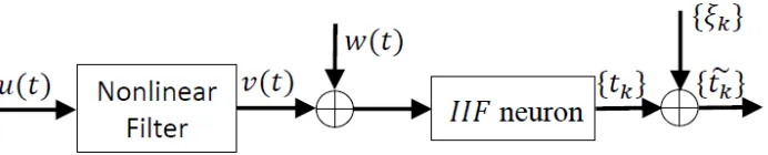
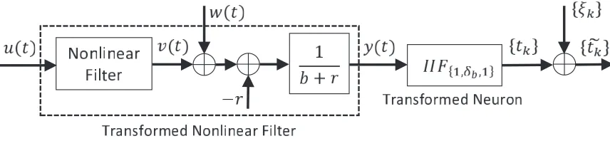
2 A new method for identifying NF-IIF circuits from spike time sequences

The proposed circuit consists of a nonlinear filter connected in series with an IIF neuron,

as depicted in Figure 1.

The nonlinear filter is described by the following equations

        

dx

dt(t) = h1(x(t), u(t)),

v(t) = h2(x(t), u(t)),

(1)

whereh1 :Rn×R→Rnandh2 :Rn×R→Rare nonlinear functions,u(t)andv(t)

are the filter input and output, respectively, andx:R_→Rnis the state variable vector.

Letx0be the initial condition of system (1).

The system (1) is assumed to have an input-output representation

dn_v

dtn =h v, v

′_{, . . . , v}(n−1)_{, u, u}′_{, . . . , u}(nu−1)_,

where1≤nu ≤n, i.e., the system is casual, andh:Rn+nu →R.

Letv0_{(t)be the response of the nonlinear filter to a step inputu}0_{(t) =A·1}

[0,∞[(t), ∀t ∈ R_, where _1[0,∞[(t) is the characteristic function of interval _[0,∞[. The filter is assumed to be bounded-input bounded-output (BIBO)-stable and that, ∀A ∈ R_{, v}0_(t)

converges to a steady state valuev0

∞, i.e., ∃limt→∞v0(t) = v∞0 . In other words, this

assumes that the system is globally asymptotically stable, which is a reasonable

as-sumption for the model of a sensory system (Smith, 2008). The filter output is assumed

to be corrupted by Gaussian white noise w(t)with zero mean and standard deviation

σw.

The IIF neuron with capacitanceC, threshold δ and bias b, denoted IIF{C,δ,b}, is

described by thet-transform equation (Lazar & Pnevmatikakis, 2008)

Z tk+1

tk

v(τ)dτ =Cδ−b(tk+1−tk), (2)

The IIF inputv(t)can be perfectly reconstructed (Lazar & Pnevmatikakis, 2011) if

v(t) >−b,∀t ∈R, _{v ∈ P WΩ} and b Cδ >

Ω

π, whereP WΩis the Paley-Wiener space of

bandwidthΩ>0

P WΩ =

v ∈L2_{(R) :supp(Fv)⊆[−Ω,Ω] ,}

whereFv(jω) is the Fourier transform of v(t) and supp(Fv) denotes the support of

Fv(jω).For a function that is not bandlimited, or whose bandwidth is unknown, there are alternative reconstruction methods available (Lazar & Pnevmatikakis, 2010; Lazar

et al., 2010).

In the following it is assumed that, for anyu(t), the output of the nonlinear filter (1)

satisfiesv ∈P WΩ,such thatΩ< _Cδπb.

The observed spike times sequence generated by the IIF neuron is assumed to be

corrupted by uniform noise{ξk}k∈Z with zero mean and amplitude A_ξ, which models

the error associated with the measurement of the spike times{tk}k∈Z.

2.1 An identification method based on an equivalent NF-IIF circuit

To simplify the identification problem, an equivalent model of the NF-IIF circuit, which

involves a single tunable parameter, is derived first. This strategy was used in (Lazar &

Slutskiy, 2010) for identifying the spiking neuron component of a LF-IIF circuit. Here,

this approach is extended to NF-IIF circuits.

Two NF-IIF circuits are said to be input-output equivalent if, given input function

u(t), they generate the same output spike times {tk}k∈Z. The equivalence relation is a consequence of the following lemma.

given inputv(t). Letr be an arbitrary number satisfyingr > −b. Then the following

holds true

Z tk+1

tk

y(τ)dτ =δb−(tk+1−tk),∀k ∈Z,

whereδb = _bCδ_+r andy(t) = v(t)−r

b+r ,∀t∈R.

Proof. Thet-transform ofIIF{C,δ,b} satisfies (2)

Z tk+1

tk

v(τ)dτ =Cδ−b(tk+1−tk) = Cδ−(b+r)(tk+1−tk) +r(tk+1−tk)

⇔

Z tk+1

tk

(v(τ)−r)dτ =Cδ−(b+r)(tk+1−tk). (3)

The required result follows after dividing both sides of (3) by(b+r).

In essence, the previous result demonstrates that the neuron IIF{C,δ,b} with input

v(t)generates the same spike times{tk}k∈Zas the neuronIIF_{1,δb,1} with inputy(t).

In practice,r =r(u)is the steady state output of the nonlinear filter in response to

a step input. As a consequence, it follows that the NF-IIF circuits depicted in Figure 1

and Figure 2 are input-output equivalent.

A method to identify the circuit in Figure 2, which involves first the identification of

the spiking neuron followed by the identification of the nonlinear filter, is summarized

below.

Step 1. Spiking neuron parameter estimation

For a given filter inputu0_{(t) = A·1}

[0,∞[(t),∀t∈R,it is assumed that the output of the NF-IIF circuit is{t0

k}k∈Z, which corresponds to the nonlinear filter outputv0(t). It is assumed that the filter input amplitudeAis selected such thatv0

∞ = limt→∞v0(t)>

Figure 2: Input-output equivalent NF-IIF circuit.

input of amplitudev0

∞. According to Lemma 1 for v(t) = v0(t) andr = v0∞, in the

absence of noise, it follows thatlimk→∞

Rtk+1

tk y(τ)dτ = 0,and thus

lim

k→∞∆t 0 k =δb,

where∆t0

k=t0k+1−t0k,∀k ∈Z.

In a more realistic scenario assuming the presence of noise and that only a finite

number of noise corrupted spike times{et0

k}Nk=1are available, an estimate of the

param-eterδbis given by

b

δb =

PN−1 k=k0∆gt

0 k

N −k0

, (4)

where k0 satisfies

g∆t0

k− N1−k

PN−1 i=k ∆gt0i

< ∆t0

err,∀k = k0, . . . , N, and ∆t0err is a

parameter selected by the user.

Step 2. Estimation and structure detection of the nonlinear filter

Let{etk}k∈Zbe the noisy output of the NF-IIF circuit given the inputu(t).The output

y(t)of the transformed nonlinear filter in Figure 2 is reconstructed from the spike times

{etk}k∈Z, assuming that they are generated by the neuron IIF_{1,δb

estimated in the previous step. The reconstruction is performed with the algorithm

introduced by Lazar & Pnevmatikakis (2010). This function reconstructed with this

algorithm is consistent, i.e., it triggers the same spike times when encoded with the

same IIF neuron and, additionally, it minimizes a smoothness criterion.

In practiceu(t)andyˆ(t)are sampled with periodε1, which is usually too small to

enable the correct identification of the nonlinear filter. For this reason, the functions

u(t)andyˆ(t)are then downsampled to periodε2 ≥ ε1 before performing system iden-tification. The value ofε2is selected using the procedure in (Billings & Aguirre, 1995),

which is known to produce improved results for identification problems.

Letu[k]andyˆ[k]be the input and output sequences of the nonlinear filter, sampled

with the period ε2. Given the input/output data, the NARMAX system identification

methodology is used to infer a NARMAX model (Leontaritis & Billings, 1981)

ˆ

y[k] =F(ˆy[k−1], . . . ,yˆ[k−ny],u[k−1], . . . , u[k−nu],

e[k−1], . . . , e[k−ne]) +e[k],

wheree[k]represents the combined effects of measurement noise, modelling errors and

unmeasured disturbances, nu, ny and ne are constants denoting the maximum input,

output and noise lags, respectively, andF : Rny+nu+ne → _R is a multivariate

poly-nomial of degreel. The structure and parameters are assumed to be unknown and are

determined using the Orthogonal Forward Regression (OFR) algorithm (Chen et al.,

1989). Specifically, given a set of candidate regressors consisting of all possible

mono-mials{pi}Mi=1, pi :Rny+nu+ne → R, a greedy iterative selection algorithm is employed

which, at each step, selects the regressor that contributes the most to the reduction of

infor-mation theoretic criterion (Akaike, 1969). The resulting model is given by

ˆ

y[k] =

m

X

s=1

θsps(X[k]) +e[k],

where

X[k] = [ˆy[k−1], . . . ,yˆ[k−ny],u[k−1], . . . , u[k−nu],

e[k−1], . . . , e[k−ne]].

To validate the model we compute the model predictions for a stimulus function

not used in identification and calculate the normalized mean squared error between the

output reconstructed with the method in (Lazar & Pnevmatikakis, 2010) and the model

predicted output (Billings, 2013)

N M SE = kyˆˆ[k]−yˆ[k]k 2 ℓ2

ky¯ˆ−yˆ[k]k2 ℓ2

,

where yˆˆ[k] is the model predicted output sequence, y¯ˆ is the average of the sequence

ˆ

y[k], andk · kℓ2 denotes the norm in spaceℓ2 .

To further evaluate the extend to which the identified nonlinear model captured the

dynamic characteristics of the system, we compute and compare the Generalized

Fre-quency Response Functions (GFRFs), of the original and identified model (Billings,

2013). The NARMAX model could also be mapped onto a continuous-time equivalent

model, for example using an approach based on the GFRFs calculated for the

NAR-MAX model (Swain et al., 1998), which would allow simulating the system at any

2.2 Numerical study

The performance of the proposed identification method is demonstrated using four

nu-merical examples.

In the first example, the nonlinear filter that satisfies the fading memory requirement,

and thus can be represented as a Volterra series, is considered. The second example

demonstrates the more general applicability of our approach, by considering a case

where the spiking neuron does not satisfy the proposed assumptions. Specifically, the

circuit consists of a nonlinear filter in series with a HH neuron (NF-HH), where the

HH neuron is connected via multiplicative coupling (Lazar & Slutskiy, 2010). The

third example considers a NF-IIF circuit where the dynamics of the nonlinear filter

are chaotic and cannot be described by a Volterra series. cannot be described by a

Volterra system. The fourth example tests the proposed methodology using input-output

recordings from a spiking neuron located in the primary visual area of the mouse.

Example 1.

The nonlinear filter block of the NF-IIF circuit is described by the following

equa-tion

v′′(t) +αv′(t) +βv(t) +γ(v(t))2 =u(t),∀t ∈R_, (5)

where α = 0.2, β = 1, γ = 0.1. The output of the nonlinear filter is corrupted by

additive Gaussian white noisew(t)with zero mean and standard deviationσw = 10−2.

The nonlinear system is connected in series with an IIF neuron with parametersb =

Step 1. Spiking neuron parameter estimation

The NF-IIF was simulated numerically using a step input u0_{(t) = 1}

[0,∞[(t) with durationT = 180s, sampled with periodε1 = 10−2s.The selected value ofT is longer

than the transient regime of the nonlinear system response. The differential equation (5)

was solved numerically to compute the nonlinear system outputv0_{(t)using theode15s}

routine in Matlab with fixed time stepε1.

The output spike train of the IIF neuron{t0

k}Nk=1, whereN = 995,is computed as

t0_k = (lk+ 1)ε1−ε1·

U((lk+ 1)ε1)−kCδ

U((lk+ 1)ε1)−U(lkε1)

, k= 1, . . . , N, (6)

whereU(lkε1) =

Rlkε1

0 (u

0_{(τ) +b)dτ is computed using the trapezoid rule, ε}

1 is the

sampling time, andlkis the unique solution of

U(lkε1)≤kCδ < U((lk+ 1)ε1).

The parameterδb was estimated fork0 = 125satisfying

∆t0

k− N1−k

PN−1 i=k ∆t0i

<

10−3_{,∀k =k}

0, . . . , N. The constantv0

∞ is estimated asv∞0 = v0(180) = 0.916.Given δ, b, C,and v∞0 ,δb

was calculated asδb = _b+Cδ_v0

∞ = 0.1885.

In this particular case, the estimation error ofδb

waseδb =δb−δˆb = 5.92·10

−7_.

Step 2. Estimation and structure detection of the nonlinear filter

The data used to identify the nonlinear filter was generated by simulating the NF-IIF

circuit using an input functionutr(t). The sampling period wasε1 = 10−2 s and the

durationT = 180s. The samples were drawn fromN(0,1). The input is subsequently

frequency 2rad/s, stopband corner frequency4rad/s, maximum attentuation in the

passband of10dB, and minimum attenuation in the stopband of40dB.The input was

subsequently normalized such that|utr(t)| ≤1.

The output of the circuit consisted of a spike time sequence {ttr

k}898k=1. To validate

the model, a separate circuit inputuval(t)and output sequence{tvalk }897k=1were generated

using the above procedure.

The output signal used to identify the filter was reconstructed first, based on the

spike time sequence{ttr

k}898k=1 and the spiking neuron model identified in step 1, and the

sampling period isε1 = 10−2s.

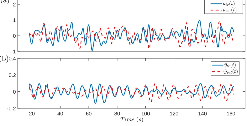
Functionsutr(t)and yˆtr(t)were preprocessed to remove the mean. To ensure that

the distortions of the reconstructed filter output due to boundary effects are not

affect-ing the identification procedure, the first and last 1800 samples were discarded. The

resulting functions are depicted in Figure 3.

The input/output data used to identify the transformed nonlinear filter was obtained

by downsampling the original data sampled atε1. The sampling period used in

identifi-cationε2 = 0.15swas determined using the approach proposed by Billings & Aguirre

(1995).

The input and output data used in identificationutr[k],yˆtr[k]was subsequently

ob-tained by downsampling the original data.

The degree of nonlinearity and the maximum number of input and output lags to

initialize the regression for the NARMAX model were determined iteratively starting

from small values. The best results in terms of prediction performance and model size

-1 0 1 2

20 40 60 80 100 120 140 160

-0.2 0 0.2 0.4

Figure 3: Filter identification and validation inputs and outputs: a) filter inputs and b)

reconstructed filter outputs.

manner, an increasing number of regressors until the stop criterionN M SE < 7·10−4_,

was met form = 10. The final set of regressors {ps(X[k])}ms=1 and the corresponding

estimated parameters{θs}ms=1 are presented in the Appendix A.

The model predicted outputyˆˆval[k], computed using the validation inputuval[k], is

shown in Figure 4a. The corresponding model prediction erroreval[k]is shown in Figure

4b. The NMSE for estimation and validation are2.52·10−4 _and2·10−4_{, respectively.}

The magnitude functions for the first and second order GFRFs for the original

sys-tem (5), derived in (Li & Billings, 2011), are given by

H1(jω) =

1

−ω2 _+αjω+β,

100 200 300 400 500 600 700 800 900 −0.1

0 0.1

0.2 yˆvalε2 [k]

ˆˆ

yε_val2 [k]

100 200 300 400 500 600 700 800 900

−2 0 2

x 10−3

Sample numberk

eval[k]

(b)

(a)

Figure 4: (a) Validationyˆval[k]and the model predicted output yˆˆval[k]. (b) The model

predicted erroreval[k].

The identified NARMAX model is used to derive analytically the first and second

order generalized frequency response functions _Hˆ_{1(jω) and H}ˆ_{2(jω1, jω2) (Billings,}

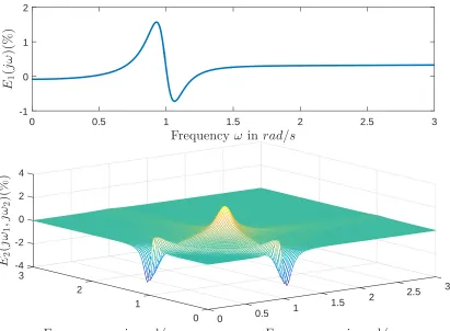
2013). The following errors are defined for quantifying the error between the GFRFs

of the original and identified transformed filter

E1(jω) = 100·

|H1(jω)| −

Hˆ1(jω)(b+v∞0 )

kH1k_∞

(%), (7)

E2(jω1, jω2) = 100·

|H2(jω1, jω2)| −

Hˆ2(jω1, jω2)(b+v0∞)

kH2k∞

(%), (8)

wherekH1k∞ = maxω∈R|H₁(jω)|andkH₂k_∞= maxω1,ω2∈R|H2(jω1, jω2)|.

The functionsH1(jω)andH2(jω2, jω2)are shown in Figure 5, and the error

0 0.5 1 1.5 2 2.5 3

Frequency ω in rad/s

0 2 4 6

|

H1

(

jω

)

|

Frequencyω2 in rad/s

|

H2

(

jω

1

,j

ω2

)

|

Frequencyω1 in rad/s

0 3 1

3

2 _2.5

2

2 1.5 3

1 ₁

0.5

0 0

Figure 5: The absolute values of the GFRF functionsH1(jω)andH2(jω1, jω2),

asso-ciated with system (5).

The NARX model was inferred from input/output measurements sampled with

pe-riod ε2 = 15·ε1, which is often too large for computing accurately the output spike

times of the NF-IIF circuit. In order to simulate the circuit with inputs utr(t), uval(t),

gener-0 0.5 1 1.5 2 2.5 3

Frequency ω in rad/s

-1 0 1 2 E1 ( jω )( % )

Frequencyω2 in rad/s Frequency ω1 in rad/s

-4 3 -2 3 0 E2 ( jω 1 ,j ω2 )( % ) 2 _2.5 2 2 1.5 4 1 ₁ 0.5 0 0

Figure 6: The error functionsE1(jω)andE2(jω2, jω2).

ated, satisfying

ui

tr[k] =utr((i+ 15k)ε1),

ui

val[k] =uval((i+ 15k)ε1), i= 1, . . . ,14.

(9)

Essentially, the filter inputs ui

tr[k], uival[k] represent the samples of u(t) measured

with periodε2, where the first sampling time isiε1,respectively. The output of the filter

for the required sampling time can then be computed by simulating the NARX model

with these inputs, for everyi, as follows.

ofyˆˆi

tr[k],yˆˆvali [k], i= 1, . . . ,15.The functions yˆˆtr(t)andyˆˆval(t), sampled withε1, were computed as

ˆˆ

ytr((15k+i)ε1) = ˆˆytri [k],

ˆˆ

yval((15k+i)ε1) = ˆˆyival[k], i= 1, . . . ,14.

(10)

Finally, the neuronIIF_{1,δˆ_b,1}generated spike time sequences{ˆttrk}719k=1and{ˆtvalk }718k=1

in response to inputsyˆˆtr(t),yˆˆval(t),respectively.

The rate of coincidence between two sequences of spike times was evaluated by

computing the coincidence factorΓ,introduced by (Jolivet et al., 2006) where

Γ = Ncoinc− hNcoinci 0.5(Ndata+Nmodel)

1 N,

whereNdata is the number of spikes in the reference spike train,Nmodel is the number

of spikes predicted by the NF-IIF model, Ncoinc is the number of coincidences with

precision∆between the two spike trains,hNcoinci= 2Nmodel∆Ndata_T1 is the expected

number of coincidences by chance, andN = 1 −2Nmodel∆_T1, where T denotes the

time duration of the simulation. The coincidence factor satisfies Γ = 1 only when

there is complete coincidence with precision∆between the predicted and the reference

spike train, respectively. Moreover, a homogeneous Poisson process with a rate equal

to Nmodel_T1 has a coincidence factor Γ = 0. The exact value for∆is not critical and,

for experimental data, Jolivet et al. (2006) introduce the constraint∆ ∈ [1ms,4ms].

For the synthetic data used in this example, we selected∆ = 0.025 s, which satisfies

∆<<0.5·min

k (t tr

k+1−ttrk) = 0.09s.

In this example, the coincidence factor wasΓtr = 1for the training data andΓval =

1for the validation data. The values correspond to a percentage of correctly predicted

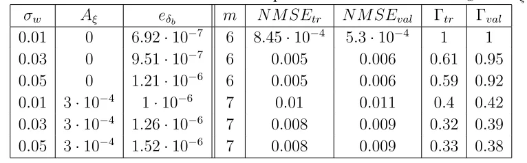
To evaluate the effect of noise on the identification method, the procedure was

car-ried out for different levels of noise applied to the filter output and the measurement of

the spike times. The results in Table 1 show thateδb is not changing significantly for

different noise levels. Because the NMSE errors are higher when the spike times are

corrupted by noise, i.e. Aξ 6= 0, the number of regressors was increased in this case to

m= 7.

Table 1: The identification results in Example 1 for different values ofσwandAξ.

σw Aξ eδb m N M SEtr N M SEval Γtr Γval

0.01 0 6.92·10−7 _{6 8.45·10}−4 _5.3·10−4 _{1 1} 0.03 0 9.51·10−7 _{6 0.005 0.006 0.61 0.95} 0.05 0 1.21·10−6 _{6 0.005 0.006 0.59 0.92} 0.01 3·10−4 _1·10−6 _{7 0.01 0.011 0.4 0.42} 0.03 3·10−4 _1.26·10−6 _{7 0.008 0.009 0.32 0.39} 0.05 3·10−4 _1.52·10−6 _{7 0.008 0.009 0.33 0.38}

Example 2.

This example demonstrates that the proposed approach can be applied to identify a

more biophysically realistic neural circuit, that does not satisfy the proposed

assump-tions. Specifically, the spiking neuron is represented as a Hodgkin-Huxley (HH) model,

given by

CdV

dt =−gN am

3_{h(V −E}

N a)−gKn4(V −EK)−gL(V −EL) +Ib

dm

dt =αm(V)(1−m)−βm(V)m dh

dt =αH(V)(1−h)−βh(V)h dn

whereV is the membrane voltage of the neuron,m, h, nare the gating variables, andIb

is the injected current. The explicit values for each parameter can be found in

(Izhike-vich, 2007). Here, the value for the injected current was chosen Ib = 120µA/cm2.

The HH equations above can be rewritten as dz

dt = f(z),where z = [V, m, h, n] and

f :R4 _→R4_.

The proposed circuit consists of a nonlinear filter, described by system (5),

con-nected via multiplicative coupling to a HH model, such that (Lazar & Slutskiy, 2010)

dz

dt = (b+v(t))f(z), (11)

whereb is a bias parameter. The output spike times {tk}k∈Z are defined as the local

maxima of the voltage tracez1(t) = V(t),such that

dz1

dt (tk) = 0, d2_z

1

dt2 (tk)<0,∀k ∈Z.

Lazar & Slutskiy (2010) have proven that the spiking neuron defined above is

input-output equivalent to the neuron model IIF{1,δ,b}, where theδ depends on the HH

pa-rameters. The new proposed methodology is used in the following for identifying an

input-output equivalent NF-IIF model for the proposed NF-HH circuit.

Step 1. Spiking neuron parameter estimation

The NF-HH circuit was excited with the same step inputu0_{(t)as in Example 1. The}

output of the filter wasv0_{(t)and the solutionz(t)of system (11) was computed using}

the ode15s routine in Matlab with fixed step ε1.The sequence of spike times {t0k}450k=1

was computed as the local maxima ofz1(t).

Step 2. Estimation and structure detection of the nonlinear filter

The identification of the nonlinear filter is carried out as in Example 1. The final set

of model terms selected for a stopping criterionN M SE < 7·10−4 _{is summarized in}

Table 5.

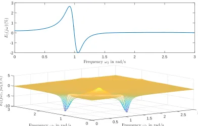
The NMSEs calculated for the training and validation data sets are5.82·10−5 _and

1.35·10−4_{, respectively. The error functionsE}

1(jω) andE2(jω), computed between the magnitudes of the GFRFs, are shown in Figure 7.

The predicted spike time sequences generated by the identified NF-IIF circuit in

re-sponse to the inputsutr(t)anduval(t)were also compared with the original ones

gener-ated by the original NF-HH model. The coincidence factors for training and validation

were Γtr = 1 and Γval = 1 respectively, corresponding to 100% correctly predicted

0 0.5 1 1.5 2 2.5 3

Frequencyω2 in rad/s -2 -1 0 1 2 3 E1 ( jω )( % )

Frequencyω2in rad/s Frequencyω1in rad/s -10 3 -5 3 2 E2 ( jω 1 ,j ω2 )( % ) 2.5 0 2 1.5 5 1 ₁ 0.5 0 0

Figure 7: The error functionsE1(jω)andE2(jω2, jω2).

Example 3.

In this example, the nonlinear filter block in Figure 1 is the well known

Duffing-Ueda chaotic nonlinear dynamical system (Duffing-Ueda, 1985)

v′′(t) +kv′(t) + (v(t))3 =u(t),∀t∈R_, (12)

wherek = 0.1. The nonlinear system is connected in series with an IIF neuron with

parametersb= 15, δ= 1.5andC= 1. In this example it is assumed thatσw =Aξ = 0.

The system (12) is solved using theode45 Matlab routine, with initial conditions

v(0) =v′_{(0) = 0.The output of the IIF neuron{t}

k}Nk=1 is computed with (6).

Step 1. Spiking neuron parameter estimation

u0_{(t) = 1}

[0,∞[(t),∀t ∈ [0, T], T = 720 s, was computed using a sampling period

ε1 = ₃₀₀π . The output of the circuit consisted of a spike time sequence {t0k}Nk=1,where

N = 7678. The noise-free data was used to estimateδˆb =δb = ∆tN0 −1 = 9.375·10−2.

Step 2. Estimation and structure detection of the nonlinear filter

An input function utr(t) = 11·cos(t) was generated, with sampling time ε1 and

duration360s.The spike time sequence generated by the NF-IIF circuit in response to

inpututr(t)was{ttrk}3582k=1.

Function yˆtr(t) was reconstructed from {ttrk}k3582=1. The functions utr(t) and yˆtr(t)

are depicted in Figure 8.

The sampling period for identification was ε2 = ₆₀π s and the original input and

output data were downsampled appropriately to generate the data set used for

identifi-cation.

The model was estimated from a set of 1771 candidate regressors corresponding

to l = 3, nu = 10, ny = 10, andne = 0. The model terms selection and parameter

estimation was performed using a final set of m = 23 regressors, input utr[k], and

outputyˆtr[k].

The selected model terms and parameters estimates corresponding to the identified

NARMAX model are presented in Appendix A, Table 4.

It is well known that chaotic systems exhibit sensitivity to the initial conditions and

thus validating them using the NMSE lacks consistency (Billings & Aguirre, 1993).

Moreover, the chaotic response doesn’t admit a Volterra series expansion, and thus

cannot be validated by computing error functions (7), (8). The bifurcation diagram

0 10 20 30 40 50 60 70 80 90 100 -10

0 10 20

utr(t)

0 10 20 30 40 50 60 70 80 90 100

Time (s)

-4 -2 0 2 4 6 8

ˆ ytr(t)

Figure 8: Filter inpututr(t)and the corresponding reconstructed nonlinear filter output

ˆ

ytr(t).

at which values A it bifurcates, and also by detecting the parameter ranges for which

the system shows chaotic behaviour (Billings & Aguirre, 1993).

The bifurcation diagrams of the true and identified nonlinear model, computed as in

4 5 6 7 8 9 10 11 1

2 3 4

Output amplitude

4 5 6 7 8 9 10 11

Input amplitude 0.05

0.1 0.15 0.2 0.25

Output amplitude

Figure 9: Bifurcation diagrams computed for the (a) original and (b) identified nonlinear

Example 4.

The proposed methodology is tested here using input-output recordings from a

neu-ron located in the primary visual area of the mouse, layer 5. The data, recorded

us-ing brain slice electrophysiology, was downloaded from the Allen Cell Type Database

(Allen Institute for Brain Science, 2015). The neuron selected has adaptation index

0.002, rheobase 390 pA, membrane time constant 7.7 ms, and firing rate 179.3 spikes/s

(Allen Institute for Brain Science, 2016). Although the database provides recordings of

the full voltage trace in response to stimuli, here only the spike times, computed as the

peak values of the voltage trace, were used in the identification procedure.

Step 1. Spiking neuron parameter estimation

To estimate the IIF parameter, we used the response of the neuron to a long square

stimulus with amplitude of 470 pA. The output spike times computed from the voltage

trace are{t0

k}Nk=1, N = 238. The neuron parameter was estimated asδˆb = 0.0044 for

k0 = 72,which satisfies|∆t0k− 1 N−k

PN−1

i=k ∆t0i|<2.2·10−3,∀k > k0.

Step 2. Estimation and structure detection of the nonlinear filter

Two different periodic stimuli of duration 1s were used for the training and

vali-dation of the model, denotedutr(t)anduval(t), consisting of pink noise with sampling

rate 200 kHz, coefficient of variation of 0.2, amplitude of 555 pA, and period 1 s.

The stimuliutr(t), uval(t)and the corresponding voltage tracesVtr(t),Vval(t), recorded

from the neuron, are depicted in Figure 10. The spike times used for the training and

validation of the filter, computed from the voltage traces, are denoted {ttr k}

Ntr

k=1} and

{tval,_k 1}Nval

0 0.5 1 200

400 600 800 1000

u_tr(t₎

0 0.5 1

200 400 600 800 1000

u_val(t₎

0.16 0.18 0.2 0.22

−0.05 0 0.05

Time (s)

Vtr(t)

0.16 0.18 0.2 0.22

−0.05 0 0.05

Time (s)

Vval(t)

Figure 10: Stimuliutr(t), uval(t)and recorded neuron voltage tracesVtr(t), Vval(t).

Given that the stimulus is periodic, in this example, the output of the nonlinear

filter (input to the IIF neuron) was reconstructed using the algorithm proposed by Lazar

et al. (2010), which uses a regularization parameterλto trade off the consistency of the

reconstruction, i.e., its ability to match the original spike times when encoded with the

same neuron, for increased smoothness. Given that the output of a biological neuron is

known to be highly corrupted by noise, this algorithm was found to give good results

for reconstructing the nonlinear filter output. After a line search algorithm, the value

λ = 10−7_{was found to lead to the smallest model predicted NMSE.}

The filter output signals used for training and validation were reconstructed based

on spike trains {ttr k}

Ntr

k=1 and {tvalk } Nval,1

k=1 , respectively. The inputs and reconstructed

0 0.1 0.2 0.3 0.4 0.5 0.6 0.7 0.8 0.9 1 −200

0 200

400 _utr(t)

uval,1(t)

0 0.1 0.2 0.3 0.4 0.5 0.6 0.7 0.8 0.9 1

−2 −1 0 1 2

Time (s)

ˆ

ytr(t)

ˆ

yval,1(t)

Figure 11: Filter input functionsutr(t), uval,1(t)and the corresponding filter responses

ˆ

ytr(t),yˆval(t), reconstructed using the method in (Lazar et al., 2010) withλ= 10−7.

The data was subsequently downsampled and processed to remove the mean. The new

sampling period isε2 = 3.5·10−3 s= 700·ε1.

The model was estimated from a set of231candidate regressor terms corresponding

to l = 2, nu = 10, ny = 10, and ne = 0. The OFR algorithm met the stop criterion

N M SE <0.23form= 4.The NARMAX model identified form the training data set

is summarized in Appendix A.

The model predicted outputyˆˆval[k], computed using the validation inputuval[k], is

shown in Figure 12a, superimposed over the output of the filter reconstructed using

the original spike-time sequence. The corresponding model prediction error eval[k]

is shown in Figure 12b. The NMSE for estimation and validation are 0.21 and 0.18,

respectively.

0 50 100 150 200 250 300 −2

−1 0 1 2

ˆ yval,1[k] ˆˆ yval,1[k]

0 50 100 150 200 250 300

−2 −1 0 1 2

Sample numberk

eval[k]

(b) (a)

Figure 12: (a) The model predicted outputyˆval[k]superimposed on the reconstructed

fil-ter output reserved for model validationyˆˆval,1[k]. (b) The model predicted erroreval[k],

computed over the validation dataset .

times prediction. For a precision of∆ = 1.5ms,the coincidence factors forttr

k andtvalk

areΓtr = 0.55andΓval = 0.48,respectively. The corresponding percentage of correctly

predicted spike times is 91.9% and 92%, respectively. These performance indicators

are in line with similar identification results for real data using simple threshold models

(Jolivet et al., 2006). Although previous work has motivated the approximation of the

subthreshold dynamics of the neuron under random current injection by a linear filter

(Jolivet et al., 2006), this example gives more insight into these dynamics, by showing

they have a significant nonlinear behaviour. This can be quantified in the proposed

model by the ERRvalue of the nonlinear regressor, i.e., its percentage contribution to

has the advantage that it requires only extracellular recordings of the neuron (the spike

times) unlike the method by Jolivet et al. (2006), that uses intracellular recordings for

3 A new method for identifying LF-LIF circuits from spike time sequences

The LF-LIF circuit (Figure 13) consists of a linear filter in series with a LIF neuron.

Figure 13: The structure of the circuit proposed for identification.

The linear filter has an impulse response function g(t) satisfying RR|g(τ)|dτ <

∞, that is, the filter is BIBO-stable. The filter gain K satisfies K = lims→∞G(s),

whereG(s)denotes the Laplace transform ofg(t).It is assumed that the filter output is

corrupted by Gaussian white noisew(t)with zero mean and standard deviationσw.

TheLIF{R,C,δ,b} neuron is described by thet- transform equation (Lazar, 2005)

Z tk+1

tk

v(τ)e−tk+1

−τ

RC dτ =C(δ−bR) +bRC·e− tk+1−_tk

RC ,∀k ∈Z, (13)

wherev(t)is the neuron input, {tk}k∈Z denotes the spike time sequence generated by

the LIF neuron,b is the bias,δis the threshold, andRandCare the neuron resistance

and capacitance, respectively.

Lazar (2005) has proven that the neuron inputv(t)can be reconstructed from the

corresponding output spike time sequence{tk}k∈Zifv ∈P W_Ωand

RC·ln

1− δ

δ−(b−c)R

Ω

π <

1−ǫ

v(t)> δ

R −b,∀t∈R, (14)

whereǫ= δ (b−c)R.

The output of the LIF neuron is assumed to be corrupted by Gaussian white noise

{ξk}k∈Z with zero mean and standard deviationAξ, which models the error associated

with the measurement of the spike times{tk}k∈Z.

3.1 An identification method based on an equivalent LF-LIF circuit

As before, the identification of the LF-LIF circuit is carried out in two distinct steps.

The first step involves the identification of the LIF neuron, which requires estimating

four parameters. By deriving an input-output equivalent LF-LIF circuit, the problem

can be simplified, requiring the estimation of only two parameters. The equivalence

relation is a consequence of the following lemma.

Lemma 2. Let {tk}k∈Z be the spike times sequence generated by neuronLIF_{R,C,δ,b}

in response to inputv(t). Letrbe an arbitrary number satisfyingr > _Rδ −b. Then the

following holds true

Z tk+1

tk

y(τ)e−tk+1

−τ

RC dτ =δ_b −RC+RC·e− tk+1−_tk

RC ,∀k ∈Z,

whereδb = _bCδ_+r andy(t) = v(_bt₊)−_rr.

Proof. Thet-transform ofLIF{R,C,δ,b} satisfies (13)

Z tk+1

tk

v(τ)e−tk+1

−τ

RC dτ =Cδ−(b+r)RC

1−e−tk+1

−_tk

RC

−r·RC1−e−tk+1

−_tk

RC

⇔

Z tk+1

tk

(v(τ)−r)dτ =Cδ−(b+r)(tk+1−tk). (15)

The previous result proves that the neuron LIF{R,C,δ,b} with input v(t) generates

the same spike times sequence {tk}k∈Z as the neuron LIF_{RC,1,δb,1} with input y(t).

In practice, r = r(u) represents, as in Section 2, the steady state output of the filter

in response to a step input. As a consequence, it follows that the circuits depicted in

Figure 13 and Figure 14 are input-output equivalent.

Figure 14: Input-output equivalent LF-LIF circuit.

A method to identify the circuit in Figure 14, which involves first the identification

of the spiking neuron followed by the identification of the transformed linear filter, is

summarized below.

Step 1. Spiking neuron parameters estimation

The following theorem establishes the basis for the estimation of the spiking neuron

parameters. Specifically, it proves that the LIF parameter RC is the unique zero of a

functionP(x) depending only on the responses of the LF-LIF circuit to a specific set

of stimuli. Moreover, the theorem proves thatP(x)takes values with opposite signs on

each side ofRC, which guarantees that the estimator converges to the true value.

Theorem 1. Let{tn k}

Nn

the LF-LIF circuit in the absence of noise, in response to the following inputs

un(t) = un_∞·1[0,∞[(t), n = 0,1,2,

whereu0

∞ =A, u1∞=A−a, u2∞=A+a, A∈Randa∈]0, aM[,aM = (

b+KA)(RC−δb)

K·RC , where K denotes the filter gain constant. Let vn_{(t) be the output of the linear filter}

component of the circuit in response to input un_{(t),and lety}n_{(t) =} vn_(t)−KA

b+KA ,forn =

0,1,2.Assuming that the linear filter is BIBO-stable and that the neuronLIF{R,C,δ,b}

satisfies condition(14), the following hold true

(a) The limitlimk→∞∆tnk = ∆tn∞exists and is finite,

where∆tn k =t

n

k+1−tnk, n= 0,1,2;

(b) The spiking neuron parameters satisfy

P(x=RC) = 0,

δb =RC

1−e−

−∆t0∞

RC

, (16)

whereP(x) = 1−e−∆tn∞

x

1−2e−∆t

1

∞

x +e−∆t

0

∞

x

− 1−e−∆t

2

∞

x

1−e−∆t

0

∞

x

,∀x >0;

(c)P(x) = 0has a unique solution;

(d) sgn(P(x)) =sgn(RC−x),∀x >0,

where sgn:R_{→ {−1,0,1}is the sign function.}

Proof. See Appendix.

The assumptiona ∈]0, aM[, aM = (b+KA_K)(_·RCRC−δb),from Theorem 1 guarantees that

the sequences∆tn

k converge forn = 0,1,2,as demonstrated in the proof. In practice, if

or more of the inputsun_{(t), n= 0,1,2.In this scenario, the requirementa ∈]0, a} M[can

be met by adjusting the valuesAanda.

The parameter RC is obtained by solving P(x) = 0 using the bisection method

(Courant & Hilbert, 1965). Specifically, the method calculates iteratively sequence

{xm}m∈N,xm = [xm,1 xm,2], where

xm+1 =

        

xm,1+xm,2

2 xm,2

, P xm,1+xm,2

2

>0,

xm,1 xm,1+₂xm,2

, P xm,1+xm,2

2

<0,

(17)

where x0,1, x0,2 ∈ Rdenote the initial conditions satisfying x0,1 < x0,2 andP(x0,1)·

P(x0,2) < 0. From Theorem 1 (d), it follows thatxm,1 < RC < xm,2,∀m ∈ N, and thus

lim

m→∞xm,i =RC,

fori= 1,2.The parameterδbis subsequently determined using equation (16).

In a more realistic scenario assuming the presence of noise and a given finite spike

times sequence{etn k}

Nn

k=1, the value∆tn∞is estimated as

d

∆tn_∞=

PNn−1

k=kn ∆gt

n k

Nn−kn

, (18)

where ∆gtn

k = etnk+1 −etnk, and kn is the index of spike time etnkn, such that, for ∀k =

kn, . . . , Nn−1,

g∆tn

k − 1 Nn−k

PNn−1

i=k ∆gt n i

<∆tn

err, where∆tnerris a parameter selected

by the user.

The neuron parameterRC is computed iteratively using (17). The stop criterion for

the iterations is given by |xm,2 −xm,1| < tol2, where tol2 denotes a tolerance value

The estimate ofδbis given by

b

δb =RCd

1−e−

d

∆t0∞

d

RC

, (19)

whereRCddenotes the estimation of the neuron parameterRC.

Step 2. Estimation and structure detection of the linear filter

Let {tk}k∈Z be the output spike times sequence generated by the LF-LIF circuit

given the inputu ∈ P WΩ,Ω > 0. The outputy(t) of the transformed linear filter is

reconstructed from the spike train{tk}k∈Zusing the method in (Lazar & Pnevmatikakis,

2010), using neuron parametersδbb,RCdcomputed inStep 1.

In practice functionsu(t)andyˆ(t)are sampled uniformly with periodε1. The data

is subsequently downsampled with periodε2, for identification purposes. Letu[k]and

ˆ

y[k] be the input and output sequences, sampled with period ε2, used to identify the linear ARMAX model

ˆ

y[k] +a1yˆ[k−1] +· · ·+anyyˆ[k−ny] =b1u[k−1] +. . . , bnuu[k−nu]

+e[k] +c1e[k−1] +· · ·+cnee[k−ne],

where e[k] is the noise variable and nu, ny, ne are the maximum input, output and

noise lags, respectively. The structure of the system is assumed to be unknown, and is

identified, as before, using the OFR algorithm (Billings et al., 1989).

3.2 Numerical study

Let G(s)be the transfer function of the linear filter component in the LF-LIF circuit,

given by

G(s) = 0.8

The output of the filter is perturbed by additive white Gaussian noise functionw(t)

with zero mean and standard deviationσw = 10−2.The linear system (20) is connected

in cascade with a LIF neuron with parametersR= 0.02, C = 1, δ= 0.02andb = 4.It

is assumed that the output of the circuit is measured with no noise, i.e.,Aξ= 0.

Step 1. Spiking neuron parameters estimation

The inputs u0_{(t) = 0, u}1_{(t) = −2· 1}

[0,∞[(t), u2(t) = 2 · 1[0,∞[(t), t ∈ [0,7 s], sampled with a period ε1 = 10−6 s, were used to generate the spike train sequences

{tn k}

Nn

k=1, n = 0,1,2, respectively, where N0 = 1216, N1 = 652, and N2 = 1776. The data was used to determine the spiking neuron parameters following the procedure

outlined in Subsection 3.1 above. The parameters∆dt0

∞= 5.8·10−3,∆dt1∞= 10.8·10−3,

and∆dt2

∞ = 3.9·10−3 were calculated using (18), where the indices kn = 1070 were

calculated for∆tn

err = 8·10−7, n= 0,1,2.

The functionP(x)and the estimated parameterdRC are depicted in Figure 15.

Al-though the function is clearly not monotonic, the bisection method is always convergent

due to Theorem 1 (d).

The spiking neuron parameters were estimated asRCd= x40,2−x40,1

2 = 0.02003(17) andδbb = 5.0008·10−3(19), wherex0 = [10−3 104]andtol2 = 10−8.

The approximation errors wereeRC =dRC−RC = 3.74·10−5andeδb =bδb−δb =

8.7·10−7_{, where, in this case,δ}

b =δ/b= 5·10−3.

Step 2. Estimation and structure detection of the linear filter

The data used to identify the linear filter was generated by simulating the NF-IIF

0 0.02 0.04 0.06 0.08 0.1

x

0 0.01 0.02 0.03 0.04

P₍x₎ d RC

Figure 15: FunctionP(x)and the estimated valueRCd.

samples are drawn from N(0,1). The input is subsequently low-pass filtered using a

Butterworth filter with bandpass corner frequency30rad/s, stopband corner frequency

50rad/s, maximum attentuation in the passband of10dB, and minimum attenuation

in the stopband of40dB.

The output of the circuit consisted of a spike time sequence{ttr

k}1214k=1. To validate

the model, a separate inputuval(t)and output sequence{tvalk }1210k=1 were generated using

the above procedure.

The data used for estimation was generated by reconstructing the input of the

spik-ing neuron (output of nonlinear filter) from {ttr

k}1214k=1 and the spiking neuron model

identified in step 1, where the sampling period is ε1. The input/output data was

pre-processed to remove the mean, and the first and last 50 samples were discarded, to

ensure that the reconstruction distortions due to boundary effects are not affecting the

identification procedure. The resulting functions are depicted in Figure 16.

ob-0 1 2 3 4 5 6 7 -1

-0.5 0 0.5 1 1.5

utr(t)

uval(t)

0 1 2 3 4 5 6 7

T ime(s)

-0.3 -0.2 -0.1 0 0.1 0.2

0.3 yˆtr(t)

ˆ

yval(t)

(a)

(b)

Figure 16: (a) The filter input functionsutr(t), uval(t)and (b) filter outputsyˆtr(t),yˆval(t)

used to estimate and validate the ARMAX model.

tained by downsampling the original data withε2 = 10−2. The maximum number of

lags used in identification arenu = ny = 10, ne = 0.The model terms selection and

parameter estimation of an ARMAX model was performed using input utr[k]and

out-put yˆtr[k]with the stop criterion N M SE < 10−3. The final set of regressors and the

corresponding estimated parameters are presented in Table 2.

Table 2: The model terms selection and parameter estimation results. Indexs Model termps(X[k]) Parameterθs ERR(%)

1 yˆ[k−1] 1.95 98.98

2 yˆ[k−2] −0.96 1.009

3 u[k−1] 2·10−3 _4.92·10−3

shown in Figure 17a. The model prediction erroreval[k] is shown in Figure 17b. The

NMSE for training and validation are3.004·10−5 _and3.23·10−5_{,respectively.}

0 1 2 3 4 5 6 7

-0.3 -0.2 -0.1 0 0.1 0.2

0.3

y

ˆ

[

k

]

ˆˆ

y

[

k

]

0 1 2 3 4 5 6 7

Lag numberk

-2 -1 0 1 2

3×10

-3

e

[

k

]

(a)

(b)

Figure 17: (a) Validationyˆval[k]and model predicted outputyˆˆval[k]. (b) Prediction error

eval[k].

iden-tified model_Gˆ_{(jω) was compared to the one of the original system. The magnitude}

frequency response function of the original systemG(jω)is shown in Figure 18a. The

magnitude error functionE1(ω)is computed (7), and depicted in Figure 18b.

100 101 102

0 0.5 1 1.5 2 2.5

|G(jω)|

100 101 102

Frequencyω (rad/s) -0.2

0 0.2 0.4 0.6 0.8

E(jω)(%)

(a)

(b)

Figure 18: (a) The magnitude frequency response functionG(jω)associated with the

linear system; (b) The magnitude error functionE1(jω).

Moreover, the identified circuit was validated in terms of the spiking output, by

simulating its response to inputsutr(t)anduval(t). In order to simulate the linear filter,

a new set of inputsuε2,i

tr [k], u ε2,i

The outputs of the linear filteryˆˆtr(t),yˆˆval(t), sampled withε1, are subsequently

com-puted from the responses of the filter with inputsuε2,i

tr [k], u ε2,i

val[k], respectively (10). The

generated output spike times were validated against the original spike time values using

the coincidence factor with precision ∆ = 0.0015 s. The values of the coincidence

factor for training and validation wereΓtr = 1andΓval = 1, respectively.

This methodology can be used for the identification of a linear filter connected via

multiplicative coupling to a Hodgkin-Huxley model (LF-HH). This results in a very

large resistance value for the LIF, which essentially turns it into a IIF model. Moreover,

the neuron identified in Example 4, Section 2, was shown to have significantly nonlinear

subthreshold dynamics, thus making it unsuitable for this methodology.

4 Conclusions

The paper introduced two novel identification methodologies for circuits consisting of

filters in cascade with spiking neurons. The first approach concerns circuits consisting

of nonlinear filters in cascade with IIF neurons. The second approach is suitable for

circuits comprising linear filters in series with LIF neurons. Compared to the

previ-ous approaches, the methods do not require a prioriknowledge of the spiking neuron

parameters or the filter structure, and do not assume that the input of the neuron (i.e.

the output of the filter) is available for measurement. Both approaches are based on

an equivalent representation of the circuit, which decreases the number of tunable

pa-rameters. The identification procedure involves two steps: the estimation of the spiking

neuron and the identification of the filter.

both proposed methodologies in the presence of additive noise applied to the output of

the filter as well as to the measured spike time sequence.

In the case of the NF-IIF circuit, the proposed identification method addresses the

well known limitations of the Volterra-based identification approaches. In particular,

the proposed approach can be used to identify NF-IIF circuits where the nonlinear filter

is not memoryless, and can even be chaotic. It is also shown that the identification

approach can be used to infer an equivalent NF-IIF model of circuits incorporating a

Hodgkin-Huxley model. The proposed identification method was also demonstrated

using a real experimental data set from the Allen Cell Type Database. It is shown that

the proposed approach can be used to identify neuron models that reproduce robustly

the experimental data.

In the case of sensory circuit models incorporating the LIF spiking neuron model,

identifying the parameters of the neuron is performed under the assumption that the

filter is linear. This allows estimating the two parameters of the equivalent LIF neuron

from the output spike time sequences corresponding to three step inputs. This method

trades off the generality of a nonlinear filter for a more general model of the spiking

neuron.

In essence, the proposed approaches allow identifying computational models that

can characterize the neural computations performed by early sensory circuits

incorpo-rating graded-potential as well as spiking neurons. These models can be connected to

models of downstream neural circuits that are identified subsequently based on

record-ings made in the downstream spiking neurons. This provides a route to constructing

Appendix A

Identification results

Table 3: The model terms selection and parameter estimation results for the nonlinear

system in Subsection 2.2, Example 1. The terms are given in the descending order of

their error reduction ratios (ERRs), which show the percentage contribution of the term

to the model output.

Indexs Model termps(X[k]) Parameterθs ERR(%)

1 yˆ[k−1] 1.12 98.01

2 yˆ[k−2] −0.56 1.96

3 u[k−1] 1.1·10−3 _8.6·10−3

4 yˆ[k−4] −0.91 3.2·10−3

5 yˆ[k−3]ˆy[k−1] −0.14 2.2·10−3

6 u[k−3] 4.4·10−3 _1·10−3

7 yˆ[k−3] 1.12 8·10−4

8 yˆ[k−5] 0.66 5·10−4

9 yˆ[k−6] −0.53 2·10−4

Table 4: The model terms selection and parameter estimation results for the nonlinear

system in Subsection 2.2, Example 2.

Indexs Model termps(X[k]) Parameterθs

1 yˆ[k−1] 3.55

2 yˆ[k−2] −4.9

3 yˆ[k−3] 2.91

4 yˆ[k−4] −0.12

5 yˆ[k−6] 0.29

6 yˆ[k−9](ˆy[k−1])2 _−0.69 7 u[k−10](ˆy[k−1])2 _9.55·10−3 8 u[k−10]ˆy[k−1]ˆy[k−2] −2.3·10−2 9 u[k−10]ˆy[k−1]ˆy[k−3] 1.39·10−2 10 u[k−7]ˆy[k−10]ˆy[k−1] −1.88·10−4 11 yˆ[k−10]ˆy[k−1]ˆy[k−2] 1.7

12 u[k−1] −9·10−5

13 (ˆy[k−1])3 −6.28

14 yˆ[k−10]ˆy[k−4]ˆy[k−2] 1.15 15 u[k−10]ˆy[k−4]ˆy[k−1] −3.05·10−4 16 yˆ[k−10] (ˆy[k−2])2 −2.41 17 yˆ[k−2](ˆy[k−1])2 _13.96 18 yˆ[k−3](ˆy[k−1])2 _−8.39

19 u[k−2] 1.68·10−4

20 yˆ[k−8](ˆy[k−1])2 _1.04

21 yˆ[k−10] −1.72·10−2

22 yˆ[k−9]ˆy[k−8]ˆy[k−3] −0.37

Table 5: The model terms selection and parameter estimation results for the nonlinear

system in Subsection 2.2, Example 3.

Indexs Model termps(X[k]) Parameterθs

1 yˆ[k−1] 6.97

2 yˆ[k−2] −23.68

3 yˆ[k−3] 51.3

4 yˆ[k−4] −78.07

5 yˆ[k−5] 86.9

6 yˆ[k−6] −71.5

7 yˆ[k−7] 42.89

8 yˆ[k−8] −17.93

9 yˆ[k−9] 4.71

10 yˆ[k−10] −0.58

11 u[k−5] −3.53·10−4

12 u[k−1] 3.68·10−4

13 u[k−2] −5.84·10−4

14 yˆ[k−10]ˆy[k−1] 4.32·10−4 15 u[k−6]ˆy[k−1] −1.84·10−5

16 u[k−10] 1.24·10−5

17 u[k−4] 6.08·10−4

18 (u[k−1])2 −1.36·10−3

Table 6: The model terms selection and parameter estimation results for the nonlinear

system in Subsection 2.2, Example 4.

Indexs Model termps(X[k]) Parameterθs ERR(%)

1 u[k−2] 0.0054 65.4

2 (u[k−2])2 −8.44·10−6 _5.43

3 u[k−3] −0.0016 4.41

4 u[k−1] 0.0995 2.53

Appendix B

Proofs of theorems

The following auxiliary lemma is used in the proof of Theorem 1 (c) and (d).

Lemma 3. LetΛz :]1,+∞[→]1,+∞[,Λz(s) = 1 1−(1−1

s)

z, z ∈]0,+∞[.

ThenΛz(s)is strictly concave forz <1, and strictly convex forz >1.

Proof. The following holds true.

Λ′_z(s) = z

s2 s s−1

z−1

2 ₋ s−1

s

z+1 2

2 =z

((s−1)s)z−1 (sz_−(s−1)z₎2,

and

Λ′′_z(s) = ((s−1)s)

z−2

h(s) (sz _−(s−1)z₎3 , where

h(s) = (z−1)(2s−1)(sz_−(s−1)z_{)−2zs(s−1)(s}z−1_−(s−1)z−1_).

It is easy to see that sgn(Λ′′

z(s)) = sgn(h(s)),∀s ∈]1,+∞[. After simple

calcula-tions, it follows that

=sz(2s+z−1)

s−1

s

z

− 2s−z−1 2s+z−1

.

To assess the sign ofh(s), the following function is evaluated

h(λ(p)) =

1 1−p

z

2

1−p +z−1 p

z₋ p(1 +z) + (1−z)

p(1−z) + (1 +z)

, (21)

whereλ:]0,1[→]1,+∞[, λ(p), 1

1−p,∀p∈]0,1[.The following holds

1 1−p

z

2

1−p +z−1

>0,∀p∈]0,1[.

Case I.z <1.

In this case p(1 +z) + (1−z) > 0,∀p, z ∈]0,1[.It follows that sgn(h(λ(p))) =

sgn(θ(p)),∀p∈]0,1[,whereθ:]0,1[→R_,

θ(p),z·ln(p)−ln

p(1 +z) + (1−z)

p(1−z) + (1 +z)

,

such thatp(1−z) + (1 +z)>0,∀p∈]0,1[.Furthermore,

θ′(p) = z

p −

4z

(p(1−z) + (1 +z)) (p(1 +z) + (1−z))

= z(1−z

2_)(p−1)2

p(p(1−z) + (1 +z)) (p(1 +z) + (1−z)).

Thenθ′_{(p)>0,∀p∈]0,1[andlim}

p→1θ(p) = 0.It follows thatθ(p)<0, h(λ(p))< 0,∀p∈]0,1[, h(s)<0,Λ′′

z(s)<0,∀s∈]1,+∞[,and thus the lemma holds true.

Case II.z >1.The following holds.

p(1 +z) + (1−z)≤0, p∈]0, p0]

p(1 +z) + (1−z)>0, p∈]p0,1[.