A CFD technique for estimating the flow distortion effects on LiDAR measurements when made in complex flow fields

A CFD technique for estimating the flow distortion effects on LiDAR measurements when made in complex flow fields

M Stickland1*, S Fabre1, T Scanlon1, A Oldroyd2 , T Mikkelson3_{, P Astrup}3

1

Department of Mechanical Engineering, University of Strathclyde, UK

2

Oldbaum Services, UK. 3

DTU Wind Energy, Denmark.

Abstract

The effect of flow distortion on the measurements produced by a LiDAR or SoDAR in close proximity to either complex terrain or a structure creating localised flow distortion is difficult to determine by analytical means. Also, as LiDARs and SoDARs are not point measurement devices, the techniques they employ for velocity measurements leads to complexities in the estimation of the effect of flow distortion on the accuracy of the measurements they make. This paper presents a method by which the effect of flow distortion on measurements made by a LiDAR in a distorted flow field may be determined using computational fluid dynamics. The results show that the error created by the flow distortion will cause the vector measured by a LiDAR to differ significantly from an equivalent point measurement. However, the results of the simulation show that, if the LiDAR is being used to measure the undisturbed flow field above a structure which creates highly localised flow distortion, the LiDAR results are less affected by the distortion of the local flow field than data acquired by a point measurement technique such as a cup anemometer.

Keywords

LiDAR, CFD, remote sensing, complex terrain,

Nomenclature

a, b, c Coefficients of equation fitted to LiDAR output ABL Atmospheric boundary layer

AMSL Above mean sea level

CTA Constant temperature (hot wire) anemometer CFD Computational fluid dynamics

EU European Union

FP7 Seventh Framework Program LiDAR Light detection and ranging Re Reynolds Number

RS Remote sensing device (LiDAR) SoDAR Sound detection and ranging

u, v, w Orthogonal components of the wind velocity vector

⃗ Free stream wind velocity vector U magnitude of free stream wind vector

Uhoriz magnitude of the free stream velocity vector in the horizontal plane

*

Corresponding author:

Dr M Stickland,

Department of Mechanical and Aerospace

Engineering,

University of Strathclyde,

Glasgow,

G1 1XJ,

UK.

Email

[email protected]

,

Tel +44 141 548 2842

Fax +44 141 552 5105

Vlos Component of the free stream vector in the direction of the laser beam

 ZephIR conical angle  ZephIR scan azimuth angle

 Free stream flow angle in horizontal plane 𝝍 Angle of the free stream to the horizontal plane

Introduction

Wind resource data is a key component for all wind energy projects. As the deadline for the EU's promised 20% reduction in carbon emissions by 2020 fast approaches, offshore wind is the key area of expansion for most EU member states in order to meet their renewable energy obligations (Bay Hasager et al 2008). However, there remain significant challenges ahead, not the least of which is the availability of good quality wind speed data to facilitate better project planning, accurate yield prediction, and a fundamentally better understanding of the offshore working environment.

To address this issue the EU, FP7 funded, NORSEWInD (North Sea Wind Index Database) project was established in order to create a wind atlas of the North, Baltic and Irish seas (FP7: the future of European Union research policy, 2012)

(Introducing: NORSEWInD, 2012). The methodology proposed by the NORSEWInD consortium was to create the wind atlas from remote sensing satellite data which was available in the public domain (Badger et al 2010, Beaucage et al 2008). However, one of the issues identified with this methodology was the extension of the satellite data, which was presented at 10m above mean sea level, to the hub height of the wind turbines likely to be deployed offshore. The hub height wind speed is required for wind resource estimation and the shear profile across the turbine blades is required for aerodynamic load assessment. On shore the extension of the 10m wind speed data would have been fairly straight forward as the shape of the shear layer over land is well understood. However, offshore the height and shape of the atmospheric boundary layer is unknown (Peña et al 2008). A number of attempts have been made to measure the shear layer offshore by mounting meteorological masts on offshore research platforms such as the FINO platforms (Neumann and Nolopp 2006) off the coasts of Denmark and Germany. These masts and the platforms they are mounted on, by their very nature, take a long time to erect and are very expensive. Also, once deployed they cannot be moved to a different location if the area of interest changes.

The NORSEWInD consortium recognised that there were available a large number of offshore platforms in the North, Irish and Baltic seas belonging to the oil and gas companies and that, by mounting instrumentation on these offshore installations, it would be possible to assess the local wind conditions and measure the maritime atmospheric boundary layer. Whilst a meteorological mast similar to those found on the FINO platforms is the accepted way of measuring the ABL there was no possibility of a similar mast being constructed on an operational offshore platform. However, the development of land based remote sensing anemometers such as LiDARs and SoDARs (Courtney et al, 2008) offered a viable alternative. With their small footprint, limited requirements for maintenance and power consumption, a number of platform operators agreed to have LiDARs located on their offshore platforms.

the distortion of the CFD generated streamlines passing over the platform shown in figure 1. The feasibility of using remote sensing devices for wind resource assessment in open terrain has been thoroughly researched in recent years. This research has led to the conclusion by Lindelow et al (2009a) that their performance is suitable for use in flat terrain. However, Lindelow (2009b) also recognised that LiDAR and SoDAR data are susceptible to interference when the flow field they are measuring is not homogeneous. Foussekis et al (2007) noted that, in a complex terrain the correlation between measurements from a meteorological mast mounted cup anemometer and a co-located LiDAR were poorer than might be expected from a similar experiment on a flat terrain. Bingol (2009) and Parmentier (2008) showed that, in complex terrain, the measurements may become biased by the distortion of the flow field caused by variation in the surrounding terrain. It was therefore deemed necessary to assess the extent of the interference of the structures, on which the NORSEWInD LiDARs were to be mounted, on the wind data acquired.

Figure 1. Streamlines over an offshore platform from CFD simulation showing distortion due to the presence of the platform. Flow from right to left in image

Methodology

The effect of flow distortion on the cup and vane type anemometer, being essentially a point measurement, is easily understood and measured. However, remote sensing devices, such as LiDARs and SoDARs, determine the wind vector from a spatially averaged set of measurements which are not easily determined analytically nor easily measured experimentally on sub scale models in wind tunnels. Some attempts have been made to measure the effect of flow distortion in complex terrain such as might be found when measuring in hilly or mountainous terrain (Bingol et al 2009) but the effect of the flow distortion on these types of devices in close proximity to large structure, such as buildings and oil rigs, had not been investigated to date.

To understand the difficulty of estimating the effect of flow distortion on the measurements made by a LiDAR it is necessary to understand the fundamental difference between the point measurement of a cup anemometer and the spatially averaged velocity measurement of a LiDAR. For clarity this paper will deal with the technique employed by the Natural power ZephIR® system. However, all LiDARs and SoDARs use a slight variation of this basic technique.

The measurement technique employed by LiDAR and SoDAR systems relies on spatially averaged line of sight velocity measurements of the flow field. To measure a 3D velocity vector three or more line of sight velocity vectors are required. Depending on the instrument and the

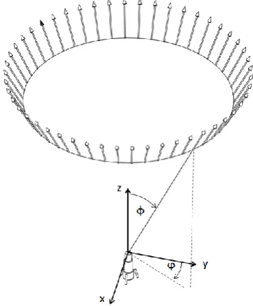
technique employed the number of measurements for each vector can be as low as 3 (AQ500 SoDAR) or as high as 50 (Natural Power ZephIR). Figure 2 shows the scanning volume for the ZephIR LiDAR, showing how, during each scan rotation, the ZephIR acquires 50 point measurements. Also included in figure 2 are the definitions of the ZephIR cone angle, ϕ, and the azimuth scan angle, φ. In order to assess the likely impact of an inhomogeneous flow field it is necessary to measure more than a single point in the flow and assess any interference that might exist at each measurement point. Only when this interference at every measurement location has been found can the effect on the final velocity vector be determined.

Figure 2. Representation of the ZephIR LiDAR Vlos vector measurement around a scan circle at the measurement height above the LiDAR.

To assess the effect of a platform’s flow distortion on the ZephIR LiDAR the flow field over each platform was simulated by Computational Fluid Dynamics. CFD was selected because, whilst wind tunnel testing is widely accepted to provide a reasonable simulation of the flow field over offshore platforms, the quantity of velocity data required from the experiment to simulate a single ZephIR measurement is, by the nature of the ZephIR measurement technique, prohibitively large. CFD allowed the flow field around each platform to be calculated and the velocity vector at any point in the flow field to be determined and therefore lent itself to the simulation of the ZephIR measurement technique.

Figure 3. 75th scale production platform model mounted in the 1.5m working section low speed wind tunnel with CTA probe located just above the platform deck.

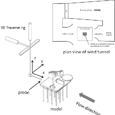
To validate the CFD model, measurements in the low speed wind tunnel were made with a calibrated DANTEC Streamline constant temperature (CTA), triple wire, hot wire anemometer mounted on a three dimensional traversing rig as shown in the diagram of figure 4. By traversing the hot wire probe vertically above the location of the simulated LiDAR the velocity profile in a vertical line above the rig could be determined. This velocity profile was then compared with the results of the CFD simulation of the rig. The uncertainty of the 3D hot wire anemometer measurement was calculated to be ±1.5% by the procedure given by Jørgenson (2002).

Figure 4. Diagram of CTA probe traverse system showing wind tunnel coordinate system and plan view of wind tunnel layout.

Initially, to create a base line against which the effect of the rig on the flow field could be assessed, the flow in the wind tunnel was traversed without the rig model present in the tunnel. The measured vectors were non-dimensionalised by a reference wind speed measured by a single hot wire probe up stream and to the right of the proposed model location, with due care taken to ensure the reference speed was outside any likely flow disturbance that might be caused by the presence of the model of the rig. This provided the non-dimensional,

undisturbed, free stream velocity at the measurement locations above the rig. The rig was then placed in the tunnel and the velocity profiles above the rig measured. Comparing this data with the data acquired in the empty tunnel the effect of the presence of the rig on the undisturbed flow field was determined. Figure 5 shows the results of four traverses above the rig with the flow approaching the rig from different azimuthal angles. The X on the plan form view of the rig shows the location above which the probe was traversed in the positive Z direction. Probe heights were normalised by the height of the rig deck (25m full scale) and the speed was normalised by the free stream velocity of the wind tunnel (15 m/s).

Figure 5. Diagram showing measured and non-dimensional velocity magnitude profiles above the platform with the flow approaching from four different azimuth angles.

It was taken that the flow was undisturbed when the magnitude of the velocity vector measured was 99% of the undisturbed value. It was then also possible, by rotating the rig through an azimuth angle, , in steps of 30o

, to plot a graph of flow angle against the height at which the flow was un-affected by the presence of the rig as measured by the hot wire probe, figure 6. For a full scale point measurement system such as a meteorological mast this data would be sufficient to determine where data was unaffected by flow distortion. However, for remote sensing systems which do not measure the velocity at a point, such as LiDARs and SODARs, the effect of the rig on the velocity measurement is not as easy to determine and requires an understanding of the way that a LiDAR measures the wind speed and direction.

Figure 6. Plot of height above rig required for 99% free stream velocity magnitude against azimuth angle using wind tunnel and CFD data

⃗ ( ) (   ) (1)

The free stream velocity vector is given by equation (2) where, , is the angle to the horizontal plane.

⃗ ( ) ( ) (2)

The projection of the wind vector on to the unit vector, calculated by the vector dot product, gives the component of the wind velocity in the direction of the laser beam, Vlos, equation (3).

   (3)

Harris (2009) also gives Vlos but in a Cartesian coordinate system with the origin situated at the LiDAR, equation (4).

_√ (4)

If the LiDAR was placed in a perfectly homogenous flow field the output of the LiDAR against azimuth scan angle would produce a rectified sine wave, as shown in figure 7, which is a plot of Vlos against scan angle for a 15 m/s flow.To calculate the velocity vector equation (5) is fitted to the waveform.

( ) (5)

Figure 7. Vlos data caclulated for a simulated LiDAR in a homogenous flowfield and a distorted flow field of 15 m/s.

The magnitude of the horizontal component of the wind vector and its angle in the horizontal plane are determined from equations (6) and (7) and the vertical component of the wind vector determined from equation (8).

_() (6)

(7)

() (8)

CFD model

The simulation was carried out by the commercial CFD code Fluent 6.3.26. The 3D model was solved using a steady state, implicit, pressure based solver on an unstructured mesh of 2.8 million cells. Mesh sensitivity was assessed by reducing cell count from approximately 7 million cells until grid independence was found. Turbulence was modelled using the two equation k-omega SST turbulence model. The k-omega turbulence model was selected because the model is a mature and established algorithm intended for general use with external flows (Menter et al, 2003). This was confirmed by comparison with a simulation using the standard k-ε model. The simulation was isothermal, steady state with inlet boundary condition defined as constant velocity of magnitude 15 m/s normal to the inlet plane with a turbulence intensity of 1% and a turbulence length scale of 0.15m. The outlet boundary condition was the standard FLUENT pressure outlet with zero gauge pressure. Convergence was defined when the sum of global residuals fell below a level of 1.e-4. Tests were conducted to see if an inlet boundary condition simulating an ABL would affect the results of the simulation but there was not found to be any effect on the final results. For inclusion in the NORSEWInD project the CFD simulation was carried out full scale and, to assess the effect of scale. The results of the simulation at full scale were compared to the wind tunnel data and there was found to be no significant difference. The Vlos data at each point in the flow field which would be scanned by a LiDAR were determined by a user defined function (UDF) in the CFD model. The user defined function was written in Microsoft visual C. The structure of the UDF was:

1. Read a settings file which passed the location of the LiDAR in the computational domain and the measurement heights above the LiDAR in the computational domain plus the zone number used by fluent to define the volume containing the fluid.

2. Interrogate the domain at the measurement locations on the scanning circle of the LiDAR. The velocity at each measurement location was found using a sequence of fluent macros. For each measurement point the cell containing the measurement point was found by the macro; c = cell_containing_point(point, ct);

where point was an array containing the measurement location in Cartesian coordinates and ct the thread containing the measurement cell. The variable, ct, was determined by the FLUENT macro

ct = Lookup_Thread(d, zone)

and d was determined from the FLUENT macro d = Get_Domain(1);

given the values for c and ct for the cell containing the measurement point the velocity components were found using the macros

u_p[0]=C_U(c,ct); u_p[1]=C_V(c,ct); u_p[2]=C_W(c,ct); 3. From the u, v and w velocity components the

Vlos was calculated using equation (3)

5. From the coefficients a, b and c the velocity vector was determined.

6. The process was repeated for the range of measurement heights required.

Results

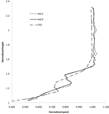
To confirm the validity of the CFD simulation and to evaluate the most appropriate turbulence model the data collected by the hot wire traverses above the rig were compared to the CFD data at the same locations. Figure 8 shows a comparison between the experimental data measured by the hot wire anemometer and the output from the CFD with the free stream aligned to 0o as defined in figure 5.

Figure 8. Comparison between point velocity magnitude calculated by CFD and experimental measurements above a platform. Lines exp a and b showing wind tunnel data repeatability

Figure 8 also shows that the repeatability of the wind tunnel data was acceptable. Lines denoted “exp a” and “exp b” were traverses of the CTA probe with the model at the same orientation but taken several weeks apart. The comparison of the experimental results and the CFD simulation data in figure 8 gave confidence that the simulation was providing a faithful representation of the flow field over the platform. The CFD simulation even picked up the wake of the crane jib, shown at a normalised height of approximately 1.3, although the cfd predicted it to be slightly larger and lower than measured by the CTA probe.

Using the simulation data it was possible to model ZephIR measurements in the computational flow field. For example, at a height of 11.25 m above the platform the ZephIR measured 50 velocity vectors at increments of 7.2o on a circle of radius 6.6m. Figure 8 shows the results of this simulation and compares the simulated ZephIR scan, created by interrogating the CFD dataset, with the theoretical measurements that would have been collected from a homogenous flow of 15 m/s.

By fitting equation 5 to this data a ZephIR system measuring at this height in the flow field would have output the results shown in table 1. Using this data it was possible to calculate the components of the measured wind vector as seen by the LiDAR and compare the ratio of the measured data to free stream wind speed with that determined at a point directly above the ZephIR at the measurement height. In all figures where data is referred

to as either point or LiDAR it refers to the method by which the data has been calculated, For point data it is the velocity data at the cell directly above the LiDAR at the measurement height and LiDAR data is the velocity calculated from the LiDAR simulation at that height.

Simulated ZephIR

Point measurement

u 14.02 m/s 14.02 m/s

v 0.41m/s 0.30 m/s

w 0.35 m/s -0.05 m/s

U 14.03 m/s 14.02 m/s

U/Ufreestream 0.94 0.93

Table 1. Comparison between point and LiDAR measurement

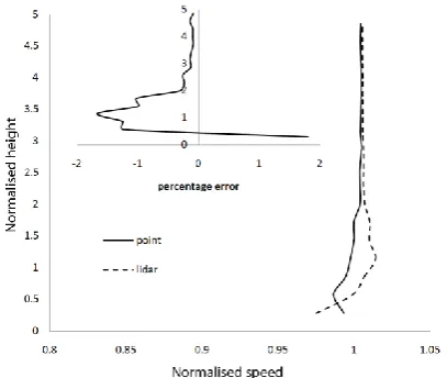
It may be seen in table 1 that, whilst the magnitude of the velocity vector has been measured reasonably well by the ZephIR, the v and w components have not. Applying the same process at a range of heights it was possible to plot velocity distributions, equivalent to a point measurement technique such as a meteorological mast, and the spatially averaged measurements from a ZephIR LiDAR above the point on the rig marked with a cross in figure 5. Figures 9 and 10 present the velocity measured by a simulated LiDAR and a point measurement for the flow approaching from angles 0o _{and 180}o _{as defined in figure 5.}

From figure 9 and figure 10 it was obvious that the LiDAR’s measurements have been affected by the flow distortion created by the platform. The amount of the distortion may be seen in the percentage error which was defined as the difference between the LiDAR and the point velocities divided by the point velocity. The errors are flow direction dependent with the ZephIR either underestimating or overestimating the point measurement value depending on wind direction and the level of flow distortion. Close to the deck of the rig, where flow distortion is significant, the difference between a point and ZephIR measurement appear to become large. This would indicate that the LiDAR would not be suitable if required to measure a point velocity within the distorted flow field at a location close to the structure. However, the requirement of the NORSEWInD project was the measurement of the undistorted free stream. In light of this requirement the results of the LiDAR simulation needed to be reassessed.

Figure 9. Comparison between results of CFD LiDAR simulation and CFD point measurement velocity magnitude with flow azimuth angle of 0o

difference between the free stream velocity magnitude and either LiDAR or point data divided by the free stream velocity magnitude. Looking at the comparison between the LiDAR result and the point measurements of free stream velocity it may be seen that the LiDAR produced a much better estimate of the free stream velocity magnitude than a point measurement in the distorted flow. This was due to the LiDAR creating its velocity measurement over a large circular region that increased with height. Therefore, the measured result was not a single point in the disturbed flow field but an averaged result which included a significant number of measurements outside the disturbed flow. This characteristic of the LiDAR measurement technique means that the volume averaged data produced a better measurement of the free stream velocity vector than a point measurement.

Figure 10. Comparison between results of CFD LiDAR simulation and CFD point measurement velocity magnitude with flow azimuth angle of 180o

Figure 11. Errors in free stream velocity magnitude measurement for LiDAR and point measurements θ=0o _left θ=180o

right

Conclusions

This paper has shown that Computational Fluid Dynamics can provide an estimate of the flow distortion on the measurements made by a ZephIR LiDAR in a distorted flow field created either by complex terrain or close proximity to large scale structures. Because of the measurement technique employed by the ZephIR, CFD was the only feasible technique that could be employed as the more conventional experimental wind tunnel tests were not feasible. The CFD simulation has shown that, if the distortion to the flow field is highly localised, such as that found near an offshore platform, the LiDAR, due to the spatial averaging in its measurement technique, will

References

Badger M, Badger J, Nielsen M, Bay Hasager C, Pena A (2010). Wind class sampling of satellite SAR imagery for offshore wind resource mapping. Journal of applied Meteorology and Climatology (49) : 2474-2491

Bay Hasager C, Pena A, Christiansen MB, Astrup P, Nielsen M, Monaldo F, Thompson D, Nielsen P (2008). Remote sensing observation used in offshore wind energy. IEEE Journal of Selected Topics in Applied Earth Observations and Remote Sensing 1(1) : 67-79

Beaucage P, Bernier M, Lafrance G, Choisnard J (2008). Regional mapping of the offshore wind resource : Towards a significant contribution from space-borne synthetic aperture radars. IEEE Journal of Selected Topics in Applied Earth Observations and Remote Sensing 1(1) : pp 48-56

Bingol F. Mann J. Foussekis D (2008). LiDAR error estimation with WAsP engineering. 14th International Symposium for the advancement of boundary layer and remote sensing. IOP Conference Series: Earth and Environmental Science 1.

Bingol F, Mann J, Foussekis D (2009). Conically scanning LiDAR error In complex terrain. Meteorologische Zeitschrift, (18) 2 : 189-195

Silva DF, Pagot PR, Gilder N, Jabardo P (2010). CFD Simulation and Wind Tunnel Investigation of a FPSO Offshore Helideck Turbulent Flow. ASME 2010 29th International Conference on Ocean, Offshore and Arctic Engineering (OMAE2010) June 6–11, 2010 , Shanghai, China

Chen Q, Gu Z, Sun T, Song S (1995). Wind environment over the helideck of an offshore platform. Journal of Wind Engineering and Industrial Aerodynamics (54–55)

February: 621–631

Courtney M, Wagner R, Lindelow P (2008). Commercial lidar profilers for wind energy. A comparative guide.

Proceedings of the European Wind Energy Conference. Brussels 2008.

Fluent User Defined Functions (2006). Fluent Inc.

Foussekis D, Mouzakis F, Papadopoulos P, Vionis P (2007). Wind profile measurements using a LiDAR and 100m mast. Proceedings of the European Wind Energy Conference, Milan.

Harris M (2009). Remote sensing for wind energy. PhD Summer School. June 2009. Risø DTU, Roskilde, Denmark,

FP7: the future of European Union research policy <http://ec.europa.eu/research/fp7/index_en.cfm>. Accessed Jan 2013

Introducing: NORSEWInD, 2012.

<http://www.norsewind.eu/public/index.html>. Accessed April 2012

Jørgensen FE (2002). How to measure turbulence with hot-wire anemometers

- a practical guide

<http://www.dantecdynamics.com/Default.aspx?ID=456>. Accessed January 2013.

Lindelow-Marsden P, Mortenson N, Courtney M (2009a). Are LiDARs good enough for resource assessment.

Internal report, Risø National Laboratory for Sustainable

Energy, Roskilde, Denmark. Available from <http://orbit.dtu.dk/services/downloadRegister/3740417/20 09_32.pdf>

Lindelow P (2009b). Uncertainties in remote wind sensing with LiDARs. R 1681(EN). Risø National Laboratory for Sustainable Energy, Roskilde, Denmark ISBN

978-87-550-3735-9 Available from

<http://orbit.dtu.dk/en/publications/upwind-d1- uncertainties-in-wind-assessment-with-lidar(94232a81-5e6f-4cdb-a5be-2a321ceedec2).html>

Menter FR, Kuntz M, Langtry R (2003), Ten Years of Industrial Experience with the SST Turbulence Model.

Turbulence, Heat and Mass Transfer 4, Begell House Inc., 2003: 625 - 632.

Natural Power’s Product Innovations (2012).

<http://www.naturalpower.com/offerings/product-innovations>. Accessed 8th April 2012.

Neuman T, Nolopp K (2006). Three years operation of far offshore measurements at FINO1. Deutsche Windenergie-Konferenz, 22 - 23 November, Bremen, Germany.

Parmentier R, Aussibal C, Ribstein B, Cariou JP, Sauvage L (2008). Accuracy and relevance of Pulsed Doppler liDAR wind profile measurement in Complex Terrain.

European Wind Energy Conference, 31 March – 3 April 2008, Brussels.

Peña A, Gryning S, Bay Hasager C (2008). Measurement and modelling of the wind speed profile in the marine atmospheric boundary layer. Boundary-Layer Meteorology (129) :479-495

Press W, Teukolsky S, Vetterling W, Flannery B (1992). Numerical Recipes in C. Cambridge University Press, New York, 683-689.