This paper is a postprint of a paper submitted to and accepted for publication at the UPEC 2014 conference and is subject to IEEE copyright. The copy of record is available at [http://dx.doi.org/10.1109/UPEC.2014.6934618].
A New Control Method for the Power Interface in
Power Hardware-in-the-Loop Simulation to
Compensate for the Time Delay.
Abstract--In an attempt to create a new control method for the power interface in PHIL simulations, a simulated PHIL sim-ulation is carried out where the simsim-ulation and hardware part are modelled in MATLAB/Simulink along with the new control method. This power interface control is proposed to achieve high accuracy in PHIL simulation with closed-loop control for aero-space, marine or micro grid applications. Rather than analyzing the Real Time Simulator (RTS) data and controlling the inter-face using time-domain resonant controllers, the RTS data will be analyzed and controlled at the interface in the frequency do-main, on a harmonic-by-harmonic and phase-by-phase basis. This should allow the RTS time delay to be compensated accu-rately, and removes the requirement to include additional com-ponents to compensate for the simulation delay into the simulat-ed power system as it is not appropriate for power systems which have short transmission lines. This is extremely relevant for marine and micro grid scenarios where such inductive com-ponents may not be present.
Index Terms--Interface algorithm, power hardware-in-the-loop (PHIL) simulation, real-time systems, simulation accuracy, simulation stability, simulation time delay.
I. INTRODUCTION
ower hardware-in-the-loop (PHIL) simulation is an ex-tension of the widely known hardware-in-the-loop (HIL) simulation concept. However, in contrast with the most common procedure of HIL called controller hardware-in-the-loop (CHIL), where the hardware under test (HUT) is a con-troller that only exchanges control signals with the simulated system, PHIL allows the testing of power components by exchanging power with the simulated system through the power interface. The power interface electrically couples and converts the low voltage/power signals of the real time simu-lator (RTS) into high voltage/power signals going into the HUT. The HUT responds to the applied signal (current or voltage), and the measurement of this response is fed back (by the power interface or an external measurement unit) to the RTS closing the loop, and therefore creating a simulation system that ideally would match with the real one. This struc-ture of a PHIL simulation is shown in Fig. 1. However, stabil-ity and accuracy issues exist when an interface is used, this is due to the introduced error during the simulation and amplifi-cation stages, and also to additional components introduced to compensate for the time-delay or for a stability improvement [1-4].
The characteristics of PHIL simulation have led to an in-creased interest in such technology, as it enables both indi-vidual power system components and full electrical systems to be tested and modelled reducing development and research costs and time. Additionally, this allows the possibility to develop experiments that otherwise would be unfeasible.
The key element of PHIL simulation is the power interface that connects the simulation section with the HUT. It is also critical for maintaining stability during the simulation and achieving high accuracy on the solution. This is due to the fact that a real power interface cannot achieve unity gain with infinite bandwidth and zero time delay, which can lead to instability or a lack of accuracy. This in turn may damage the HUT. There must be a conservation of energy across this in-terface, but there will also be a time delay between the simu-lation and HUT which will lead to a phase difference between the HUT and the simulation model.
To avoid the system instability caused by the introduction of a time delay in the interface, one option could be to carry out the simulation with open-loop control. However this leads to the loss of accuracy and to an incomplete PHIL simulation [5]. Overcoming the delay by introducing additional compo-nents into the simulated power system to compensate for the delay (transmission lines or transformers) is not appropriate for power systems which have short transmission lines; for example marine, aerospace or micro grid power systems. Ar-tificially increasing the line impedance to increase system stability for such systems would therefore result in a dynamic response, which would not be representative of the actual electrical power system. Other approaches of compensation described in the literature are a “Lead” block before the am-plification and an extrapolation prediction [6], a low pass
E. Guillo-Sansano
University of Strathclyde [email protected]
A.J. Roscoe
University of Strathclyde [email protected]C.E. Jones
University of Strathclyde [email protected]G.M. Burt
University of StrathclydeMember IEEE [email protected]
P
This paper is a postprint of a paper submitted to and accepted for publication at the UPEC 2014 conference and is subject to IEEE copyright. The copy of record is available at [http://dx.doi.org/10.1109/UPEC.2014.6934618].
filter in the feedback signal [7,8], and also a phase shift of the feedback signal [9].
In this paper a method to compensate for the time delay similar to those presented on [9,10] is presented, however the RTS data will be analysed and controlled at the power inter-face in the frequency domain, on a harmonic-by-harmonic and phase-by-phase basis, allowing the RTS time delay to be compensated accurately by advancing the phase of the signal in the frequency domain and reconstructing the signal into time domain before its amplification, as shown in Fig. 1. With this new control in the power interface, the requirement to include additional components to compensate for the simu-lation delay into the simulated power system is removed. Al-so an improvement on the accuracy of PHIL simulation is expected when the time-delay is compensated.
II. POWER INTERFACE ALGORITHM
A Power-HIL simulation can be divided in three main sec-tions:
Simulated system Power interface Hardware under test
However, the most important part of the PHIL simulation is the power interface as is the one responsible for the accuracy and stability of the simulation. This is due to the fact that the power interface is the component that makes the power HIL different from the original circuit in order to connect software and hardware and at the same time amplify the signal from the simulation to a high voltage/power signal.
The power interface can be implemented with different methodologies; these different topologies of the power inter-face are called interinter-face algorithms (IA). Five different IAs have been reported in the literature, where the stability and accuracy of the algorithms have been studied with linear and non-linear HUT [11]. From the five IAs only two of them presented suitable stability and accuracy characteristics to be implemented in a real PHIL simulation (the most commonly used ones), these are the ideal transformer model (ITM) and the damping impedance method (DIM) algorithms.
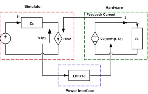
For the scope of this paper, the simulation studies have been carried out with the ITM interface, as it is the only rithm that avoids the linking inductive component (DIM algo-rithm requires a linking component), as it is shown in Fig. 2. Therefore this is a suitable interface for marine and aero sys-tems, and alongside this it is closer to an ideal interface (one without linking component or time delay).
The ITM interface is commonly used in practical PHIL simulations because of its straightforward implementation and proven good stability and accuracy during simulation [1,8]. There exist two different topologies of the ITM depend-ing on which signal is amplified (current or voltage), in this case we have used the voltage type. A structure of PHIL sim-ulation with a voltage type ITM interface algorithm is shown in Fig. 3.
An analysis of the stability of the interface algorithm is recommended before implementing a PHIL simulation, how-ever the exact characteristics of the HUT required to carry out a stability test, will seldom be known before the simulation. Otherwise if the characteristics are known a complete com-puter simulation could be performed and a PHIL simulation would not be required.
In this case a linear load has been considered as the HUT to perform the analysis of the stability of the ITM interface. The equivalent control diagram of the PHIL simulation is shown in Fig. 4. For the analysis of the stability the power interface is assumed to be ideal with unity gain but with a time delay (Td) in the voltage amplification.
With this assumption, the open loop transfer function can be derived as:
( )( ) (1)
The stability of the system will depend on ZS/ZL as the time
delay on the frequency domain represents constant decrease of the phase for an increasing frequency. At this point, a Nyquist plot of the system open loop transfer function (1) will show that for ZS/ZL>1 the system will become unstable
because the point (-1,0) will be encircled, but when ZS/ZL<1
[image:2.595.305.550.55.191.2]the system will be stable.
Fig.2. ITM interface and DIM interface algorithms.
[image:2.595.305.549.213.368.2]This paper is a postprint of a paper submitted to and accepted for publication at the UPEC 2014 conference and is subject to IEEE copyright. The copy of record is available at [http://dx.doi.org/10.1109/UPEC.2014.6934618].
III. TIME DELAY COMPENSATION METHOD
In a power HIL simulation different time delays have to be accounted for, with the time delay introduced by the power interface being the most significant. Other delays are intro-duced by the A/D and D/A devices and the RTS simulation. The time delay introduced leads to an inaccurate system and can also affect to the stability system in some cases. It also could cause a change in the power factor of the system [7], affecting to the behaviour of different devices that their active and reactive power consumption/generation depend on the power factor of the system.
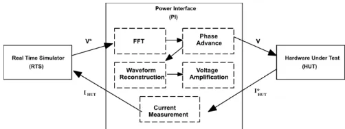
This time delay of an AC signal is equivalent to a phase shift in the frequency domain, so the method proposed to compensate for this time delay (Fig.5) will decompose the signal from the RTS with an FFT transforming the time main signal into the frequency domain. In the frequency do-main a phase advance of the signal is added to the fundamen-tal and harmonics analysed to compensate for the time delay of the system. After the compensation takes place, the signal is reconstructed and can be accurately amplified by the power interface. Reference [7] presents a similar method for com-pensation, however the compensation is carried out in the feedback path and the algorithm is limited by using a fixed frequency for the process. In this new algorithm a variable frequency is used. The main limitation of an FFT based algo-rithm is that it is not appropriate for fast transients as it is not predicting the future (no controller can predict the future). In addition the computation time of an FFT has to be taken into account: only a definite number of harmonics can be pro-cessed to simulate the system in real time. Hence, this will have an impact on the accuracy although if enough harmonics are processed, then the impact on accuracy will be minor.
This compensation methodology has been selected due to its capacity to compensate the accumulated time delay of the system avoiding inserting additional components to the sys-tem that would modify the dynamic behaviour of the original system under test. Therefore, it can be expected that with the implementation of this new algorithm the accuracy of the ITM interface can be greatly improved and the applicability of PHIL can be extended to modelling scenarios such as ma-rine and aero power systems, low-voltage distribution net-works or micro grids. For these systems the removal of the inductive components used to link hardware and software or to compensate for the time delay was essential.
In such scenarios the current (and voltage) waveforms may contain significant harmonics, and the proposed method should allow the phase relationships of these harmonics to be
maintained on both sides of the interface (i.e. in simulation and hardware). The phase relationship of the fundamental voltages and currents of course relate to the power angle (power factor), but the harmonic relationships may be equally important.
IV. SIMULATION SCENARIOS
To date the algorithm has been tested using software simu-lation, where the HUT and power interface are modelled in the simulation software (Matlab/Simulink). A simplified PHIL scenario (a voltage divider system) is modelled where the HUT is represented as a linear load, the power interface is modelled only as a time delay and therefore assuming that it has unity gain, the simulated network is also modelled in Simulink and is composed of a voltage-source and a source-impedance. For the simulation with the compensation method the developed FFT and compensation algorithm are intro-duced in the voltage presented to the power interface.
A. Original scenario without interface
First of all a simulation of the real scenario, where there is no interface, is executed in order to have an original signal to be compared with. The original scenario consists of a 1pu, 50Hz voltage source that will be disturbed with a 0.1pu, 250Hz signal. From previous calculations performed in sec-tion II, it is known that when ZS/ZL>1 the system will become
unstable, so for the simulation ZS=2Ω and ZL=5Ω satisfying
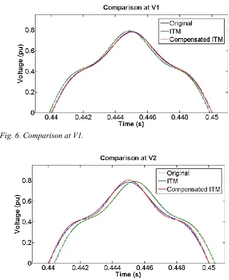
the stability criteria. No time delay is present in this simula-tion as it is ideally coupled without interface. The original signal that arises from this scenario is shown in Fig. 6 as “Original”.
B. PHIL with ITM interface
This scenario is shown in Fig.3. The power interface is as-sumed ideal and therefore with unity gain although a time delay of 500µs is assumed to be present at the interface and a simulation time step of 50µs. To maintain the equivalence between the systems and to be able to compare them, the re-maining values of the system are the same as the ones used with the original system scenario presented in section A.
[image:3.595.45.290.54.138.2]C. PHIL with ITM interface and time-delay compensation The proposed time-delay compensation is added to the power interface in this scenario. The parameters are still the
Fig. 4. Block diagram of the PHIL simulation with ITM interface.
[image:3.595.305.556.56.150.2]This paper is a postprint of a paper submitted to and accepted for publication at the UPEC 2014 conference and is subject to IEEE copyright. The copy of record is available at [http://dx.doi.org/10.1109/UPEC.2014.6934618].
same as in the other scenarios and no new parameters are added because the compensation is just processing the signal and phase-shifting it to cope with the time delay. The phase shift angle in this case will be fixed and equal to the 500µs time delay existing in the system.
V. RESULTS
A comparison between the ITM interface algorithm and the ITM with time–delay compensation algorithm has been car-ried out. Figs. 7-9 show comparisons of V1 and V2 in the time domain, since this is the simplest and most convenient way to show them in this paper. This comparison is valid for the simple example case shown, where the time delays are all considered to be lumped within the interface. In a more gen-eral PHIL application, the total closed-loop time delays are distributed, including contributions from simulation, sam-pling of HUT currents, and communication/samsam-pling of simulated voltages from RTS to the interface. In those more complex (and real) PHIL scenarios, accuracy of the PHIL environment can be assessed by monitoring how well the wave shapes are reproduced on both sides of the interface, and how well the phase relationships between currents and voltages are preserved on either side of the interface. “Per-fect” PHIL implementation would result in the following properties:
In the case of the fundamental, the power angle (power factor) must be preserved at both sides of the interface.
The voltage and current wave shapes must be identical on either side, i.e. the harmonic amplitude and phase relationships between voltage harmonics and funda-mental must be preserved, and similarly for currents.
The phase relationships between currents and voltages (the power angles of the harmonics) must be main-tained at both sides of the interface.
However, while all the above conditions must be met for a “perfect” interface, V1 and V2 (and I1 and I2) will be ex-pected to be out of phase with each other due to the finite delays in sampling and simulation. So, while a direct compar-ison of V1 and V2 has been made in this paper, in the more general PHIL context a more complex measure of accuracy will be required.
Therefore, to analyse how these conditions are met differ-ent comparisons have been performed.
1. Comparison at V1
Fig. 6 shows a comparison between voltages at V1 between the original system, the PHIL with ITM interface and the ITM interface with time-delay compensation that have been presented in section IV. From inspection of the graph it is clear that the accuracy of the compensated ITM voltage waveform at V1 is improved with respect to the usual ITM voltage waveform and it is also really close to the behaviour shown by the original system. It is also noticeable that no time delay exists between the compensated ITM and the
orig-inal voltage, however the ITM algorithm has a different phase angle.
2. Comparison at V2
As important as the voltage shown at V1 is the voltage at V2 because this is the voltage that the HUT will respond to. Hence, depending on voltage V2 the response of the HUT (the feedback current) can change. Fig. 7 shows the behaviour of the voltage V2 in the different scenarios, where the com-pensated ITM algorithm demonstrates the improvement in accuracy compared with the ITM interface. Although in this case the compensated ITM does not match exactly the origi-nal waveform, for ZS/ZL<<<1 the compensated ITM
algo-rithm can match exactly the original waveform.
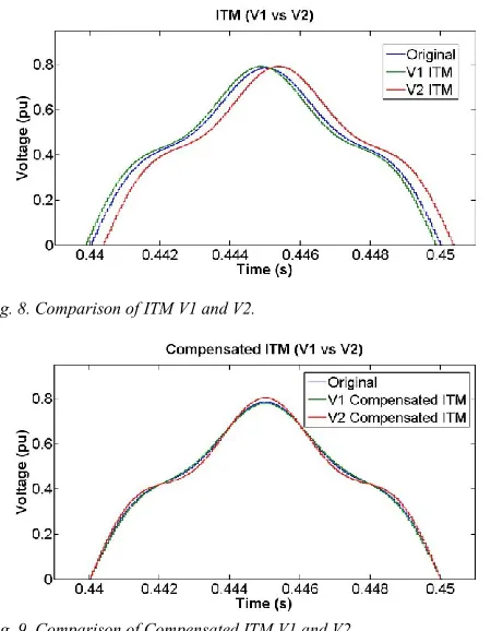
3. Comparison of ITM V1 and V2.
In order to achieve an accurate PHIL simulation high levels of similarity are required between the voltages on both sides of the interface. The ITM algorithm presents a large differ-ence between V1 and V2 due to the time-delay introduced in the system, as shown in Fig. 8. This difference between the voltages leads to a phase difference in the system that can produce very different behaviours of systems with reactive power characteristics due to the change of the power factor.
4. Comparison of Compensated ITM V1 and V2
[image:4.595.305.534.55.335.2]Fig. 9 shows the behaviour of the compensated ITM algo-rithm, where voltages V1 and V2 are very similar between them and at the same time similar to the original system volt-age as the time delay introduced by the interfaced system has
Fig. 6. Comparison at V1.
This paper is a postprint of a paper submitted to and accepted for publication at the UPEC 2014 conference and is subject to IEEE copyright. The copy of record is available at [http://dx.doi.org/10.1109/UPEC.2014.6934618].
been compensated. It is clear that the accuracy of the com-pensated ITM algorithm has been improved compared with the ITM interface presented before.
VI. CONCLUSIONS
A new method to compensate for the time-delay in the power interface of a PHIL simulation has been proposed in this paper. By compensating for the time-delay it has been shown that the accuracy is greatly improved, when compared with the commonly used ITM interface. With the implemen-tation of this methodology the addition of linking impedances or the simulation of a large inductive component in the RTS is no longer necessary. Therefore a new opportunity to im-plement accurately a PHIL simulation has arisen for marine, aerospace or micro-grid systems which have short lines and hence low levels of line impedance.
REFERENCES
[1] De Jong, E., et al. European White Book on Real-Time Power Hardware in the Loop Testing. DERlab, 2012.
[2] Viehweider, A., G. Lauss, and F. Lehfuss. “Stabilization of Power Hardware in the Loop Simulations of Electric Energy Systems.”
Simulation Modelling Practice and Theory, 2011: vol.19, Issue 7, pp. 1699-1708.
[3] Kotsampopoulos, P., V. Kleftakis, G. Messinis, and N. Hatziargyriou. “Design, Development and Operation of a PHIL Environment for Distributed Energy Resources.” IEEE Industrial Electronics Society.
2012. 4765 - 4770.
[4] Dargahi, M., A. Ghosh, G. Ledwich, and F. Zare. “Studies in Power Hardware in the Loop (PHIL) Simulation Using Real-Time Digital Simulator (RTDS).” Power Electronics, Drives and Energy Systems.
IEEE, 2012. 1-6.
[5] Hong, M., S. Horie, Y. Miura, T. Ise, and C. Dufour. “A Method to Stabilize a Power Hardware-in-the-Loop Simulation of Inductor Coupled Systems.” Power System Transients. 2009.
[6] Ren, W., et al. “Interfacing Issues in Real-Time Digital Simulators.”
IEEE Trans. Power Delivery. 2011. vol.26, no.2, p. 1221-1230. [7] Ren, W., M. Steurer, and S. Woodruff. “Applying Controller and
Power Hardware-in-the-Loop Simulation in designing and Prototyping Apparatuses for Future All Electric Ship.” Proc. IEEE Electric Ship Technologies Symp. 2007.
[8] Ren, W., M. Steurer, and T.L. Baldwin. “Improve the Stability and Accuracy of Power Hardware-in-the-Loop Simulation by Selecting Appropriate Interface Algorithms .” IEEE Trans. Industry Applications. 2008. vol. 44, no.4, pp. 1286-1294.
[9] Roscoe, A., A. Mackay, G. Burt, and J. McDonald. “Architecture of a Network-in-the-Loop Environment for Characterizing AC Power-System behavior.” IEEE Trans. Industrial Electronics. 2010. vol.57, no.4, pp. 1245-1253.
[10] Steurer, M., C. Edrington, M. Sloderbeck, W. Ren, and J. Langston. “A Megawatt-Scale Power Hardware-in-the-Loop Simulation Setup for Motor Drives.” IEEE Trans. Industrial Electronics. 2010. vol.57, no.4, pp. 1254-1260.
[11] Viehweider, A., G. Lauss, and F. Lehfub. “Stabilization of Power Hardware-in-the-Loop Simulations of Electric Energy Systems.”
[image:5.595.48.273.48.337.2]Simulation Modelling Practice and Theory. 2011. vol.19, no.7, pp. 1699-1708.
Fig. 8. Comparison of ITM V1 and V2.