Almost sure exponential stability in the numerical simulation of stochastic differential equations

ALMOST SURE EXPONENTIAL STABILITY IN THE NUMERICAL

SIMULATION OF STOCHASTIC DIFFERENTIAL EQUATIONS∗

XUERONG MAO†

Abstract. This paper is mainly concerned with whether the almost sure exponential stability of stochastic differential equations (SDEs) is shared with that of a numerical method. Under the global Lipschitz condition, we first show that the SDE ispth moment exponentially stable (forp∈(0,1)) if and only if the stochastic theta method ispth moment exponentially stable for a sufficiently small step size. We then show that thepth moment exponential stability of the SDE or the stochastic theta method implies the almost sure exponential stability of the SDE or the stochastic theta method, respectively. Hence, our new theory enables us to study the almost sure exponential stability of the SDEs using the stochastic theta method, instead of the method of the Lyapunov functions. That is, we can now carry out careful numerical simulations using the stochastic theta method with a sufficiently small step size Δt. If the stochastic theta method ispth moment exponentially stable for a sufficiently smallp∈(0,1), we can then infer that the underlying SDE is almost surely exponentially stable. Our new theory also enables us to show the ability of the stochastic theta method to reproduce the almost sure exponential stability of the SDEs. In particular, we give positive answers to two open problems, (P1) and (P2) listed in section 1.

Key words. almost sure exponential stability, moment exponential stability, stochastic theta method, Lipschitz condition, linear growth condition

AMS subject classifications.65C30, 60H35

DOI.10.1137/140966198

1. Introduction. Stochastic differential equations (SDEs) have been widely used in many branches of science and industry with the emphasis being on stabil-ity analysis [1, 6, 11, 13, 16]. One of the most powerful techniques in the study of stochastic stability (e.g., the moment exponential stability or almost sure exponen-tial stability) is the method of Lyapunov functions. Suppose that we are required to find out whether an SDE is stochastically stable. In the absence of an appropriate Lyapunov function, we may carry out careful numerical simulations using a numerical method with a “small” step size Δt. We are then left with two key questions:

(Q1) If the SDE is stochastically stable (e.g., mean square exponentially stable or almost surely exponentially stable), will the numerical method be stochastically stable?

(Q2) If the numerical method is stochastically stable for smallΔt, can we infer that the underlying SDE is stochastically stable?

There are various types of stochastic stabilities, including the exponential stability in mean square, almost sure exponential stability, and asymptotic stability in probability [11, 14, 15]. In any case, both questions (Q1) and (Q2) deal with asymptotic (t→ ∞) properties and hence cannot be answered directly by applying traditional finite-time convergence results.

∗_{Received by the editors April 23, 2014; accepted for publication December 3, 2014; published} electronically February 3, 2015. This work was supported by the EPSRC (EP/E009409/1), the Royal Society of London (IE131408), the Royal Society of Edinburgh (RKES115071), the London Mathematical Society (11219), the Edinburgh Mathematical Society (RKES130172), and the State Administration of Foreign Experts Affairs of China (MS2014DHDX020).

http://www.siam.org/journals/sinum/53-1/96619.html

†_{Department of Mathematics and Statistics, University of Strathclyde, Glasgow G1 1XH, UK} ([email protected]).

In the case where stochastic stability means exponential stability in mean square, results that answer (Q1) and (Q2) for scalar, linear systems can be found in [7, 20, 21]. Baker and Buckwar [3] consider the stability of numerical methods for scalar constant delay SDEs under the assumptions of the global Lipschitz coefficients and the existence of a Lyapunov function. Schurz [21] also has results for nonlinear SDEs. In particular, for nonlinear SDEs under the global Lipschitz condition, Higham, Mao, and Stuart [9] show that the exponential stability in mean square for the SDE is equivalent to the exponential stability in mean square of the numerical method (e.g., the Euler– Maruyama and the stochastic theta method) for sufficiently small step sizes. For further developments in this area, we refer the reader to [5, 8, 19, 22, 24, 27], for example, and the references therein.

In the case where stochastic stability means almost sure exponential stability, so far most results answer (Q1), but few address (Q2). In fact, unlike in the mean square case, the first paper that addressed these questions on a reasonable class of SDEs was Higham, Mao, and Stuart [10] in 2007. In their paper, they answered (Q1) and (Q2) for the linear scalar SDE using the Euler–Maruyama method. For the nonlinear SDE, they answered (Q1) using the Euler–Maruyama method for the SDE under the linear growth condition plus the additional condition which guaranteed the almost sure exponential stability of the SDE. For the nonlinear SDE without the linear growth condition, they answered (Q1) using the backward Euler method. The research in this area has since then been developed by many authors, e.g., [4, 17, 25, 26], but all of these authors have addressed (Q1). There are many open problems in this direction. Two of them are stated below:

(P1) If the multidimensional linear SDE

(1.1) dy(t) =A₀y(t)dt+ m

i=1

A_iy(t)dw_i(t)

is almost surely exponentially stable, will a numerical method be almost surely exponentially stable for all sufficiently small step sizes?

(P2) Under the conditions in Theorem 4.5 below, the nonlinear SDE (2.1) is almost surely exponentially stable. This theorem is one of the most useful criteria on almost sure exponential stability. However, will a numerical method be almost surely exponentially stable for all sufficiently small step sizes? Should we have some answers to (Q1) and (Q2) in the case where stochastic stability means almost sure exponential stability, these problems would be solved to a certain degree. In this paper we will address (Q1) and (Q2) in the sense of almost sure exponential stability in two steps. Under the global Lipschitz condition, we first show that the SDE is pth moment exponentially stable (for p∈(0,1)) if and only if the stochastic theta method ispth moment exponentially stable for a sufficiently small step size. We will then show that the pth moment exponential stability of the SDE or the stochastic theta method implies the almost sure exponential stability of the SDE or the stochastic theta method, respectively. Hence, our new theory enables us to study the almost sure exponential stability of the SDEs using the stochastic theta method instead of the method of the Lyapunov functions. That is, we can now carry out careful numerical simulations using the stochastic theta method with a sufficiently small step size Δt. If the stochastic theta method ispth moment exponentially stable for a sufficiently smallp∈(0,1), we can then infer that the underlying SDE is almost surely exponentially stable. Our new theory also enables us to show the ability of the stochastic theta method to reproduce the almost sure exponential stability of the

SDEs. In particular, we will be able to solve problems (P1) and (P2). In fact, it is known (see, e.g., [2]) that the linear SDE (1.1) is almost surely exponentially stable if and only if it ispth moment exponentially stable for a sufficiently smallp∈(0,1). Moreover, under the conditions of Theorem 4.5, we will show that the nonlinear SDE (2.1) ispth moment exponentially stable for a sufficiently smallp∈(0,1). Applying our new results, we will hence have the positive results on both (P1) and (P2).

Before we proceed to establish our new theory, we should point out that the way we establish our new results on (Q1) and (Q2) in the sense of the pth moment exponential stability for sufficiently smallp∈(0,1) is motivated by our earlier paper [9] that deals with the 2nd moment exponential stability. However, there are at least two significant differences which we highlight below:

• It was assumed in [9] that a numerical method is available which, given a step size Δt > 0, computes discrete approximations x_k ≈y(kΔt), with x₀ =y₀. It was also assumed that there is a well-defined interpolation process that extends the discrete approximation{x_k}_k∈Z+ to a continuous time

approxi-mation{x(t)}_t∈R+, withx(kΔt) =x_k. However, in general, only the discrete

approximationsx_k are computable but not the continuous-time approxima-tion {x(t)}_t∈R+. It is therefore more useful in practice if the theory is only

based on the discrete approximationsx_k,and this is what we will establish in this paper. In other words, in this paper, we only need a numerical method which computes the discrete approximations x_k ≈ y(kΔt), and we do not require the continuous-time approximations.

• Mathematically speaking, many inequalities used in [9] for the 2nd moment do not work for the pth moment when p∈(0,1). We therefore have to develop new techniques to handle the pth moment. Moreover, our new theory is based on the discrete approximationsx_k, so we have to apply the discrete-time analysis in many proofs in this paper, while [9] used the continuous-discrete-time analysis essentially.

2. pth moment exponential stability.

2.1. Stochastic differential equations. Throughout this paper, we let (Ω,F,

{Ft}t≥0,P) be a complete probability space with a filtration {F_t}_t≥0 satisfying the usual conditions (i.e., it is right continuous and increasing whileF₀contains allP-null sets). Letw(t) = (w₁(t), . . . , w_m(t))T be anm-dimensional Brownian motion defined on the probability space. Let| · |denote both the Euclidean norm inRn and the trace norm in Rn×m. For a, b ∈ R, we use a∨b and a∧b for max{a, b} and min{a, b}, respectively.

Consider ann-dimensional Itˆo SDE

(2.1) dy(t) =f(y(t))dt+g(y(t))dw(t)

ont≥0 with initial valuey(0) =y₀∈Rn, where

f :Rn→Rn and g:Rn →Rn×m.

Throughout this paper, unless otherwise specified, we impose the following assumption as a standing hypothesis.

Assumption 2.1. Both f andg satisfy the global Lipschitz condition. That is, there is a positive constant K such that

(2.2) |f(x)−f(y)| ∨ |g(x)−g(y)| ≤K|x−y| ∀x, y∈Rn.

Moreover,f(0) = 0 andg(0) = 0.

We should point out that the reason we assume that f(0) = 0 and g(0) = 0 is because this paper is concerned with the stochastic stability of the trivial solution

y(t)≡0. It is also easy to see that this assumption implies the linear growth condition (2.3) |f(y)| ∨ |g(y)| ≤K|y| ∀y∈Rn.

Moreover, it is well known (see, e.g., [1, 6, 16]) that under Assumption 2.1, the SDE (2.1) has a unique global solutiony(t) ont≥0 and the solution satisfies

(2.4) E|y(t)|p≤H(t, p, K)|y₀|p, t≥0,

for any p >0, where H(t, p, K) is a positive constant dependent on t, p, K only. In this paper, it is useful to haveH(t, p, K) explicitly forp∈(0,1). It is straightforward to show that

E|y(t)|2≤3|y₀|2+ 3K2(t+ 1)

_t

0 E|

y(s)|2ds.

This, by the Gronwall inequality, yields

E|y(t)|2≤3|y₀|2e3K2t(t+1).

(2.5)

Hence, whenp∈(0,1),

E|y(t)|p≤(E|y(t)|2)p/2≤3p/2e1.5pK2t(t+1)|y₀|p.

In other words, we have

H(t, p, K) = 3p/2e1.5pK2t(t+1)

(2.6)

forp∈(0,1).

Of course, we may consider a more general case, for example, where the SDE has its random initial data y(0) = ξ which is an F₀-measurable Rn-valued random variable such that E|ξ|p < ∞ ∀p > 0. In this case, by the Markov property of the solution, we can easily see that the solution satisfies

(2.7) E|y(t)|p=E(E(|y(t)|p|ξ))≤E(H(t, p, K)|ξ|p) =H(t, p, K)E|ξ|p, t≥0,

∀p >0. It is therefore clear why it is enough to consider only the deterministic initial valuey(0) =y₀∈Rn. Moreover, for any t₀≥0, we can regardy(t) on t≥t₀ as the solution of the SDE (2.1) on t≥t₀ with initial data y(t₀) at t=t₀. As the SDE is time-homogeneous, we hence see from (2.7) that

(2.8) E|y(t)|p≤H(t−t₀, p, K)E|y(t₀)|p, t≥t₀,

for anyp >0. In this section we consider thepth moment exponential stability of the origin, which we define as follows (see, e.g., [6, 11, 14, 15]).

Definition 2.2. Let p >0. The SDE (2.1)is said to be exponentially stable in

thepth moment if there is a pair of positive constantsλandM such that, for every initial valuey₀∈Rn,

(2.9) E|y(t)|p ≤M|y₀|pe−λt ∀t≥0. We refer to λas a rate constantandM as a growth constant.

As in the explanation of (2.8) we see that (2.9) is equivalent to the following more general form:

(2.10) E|y(t)|p ≤ME|y(t₀)|pe−λ(t−t0) _∀t≥t

0≥0.

2.2. Numerical solutions. We suppose that a numerical method is available which, given a step size Δt >0, computes discrete approximationsx_k ≈y(kΔt) for

k ∈ Z+ with x₀ = y₀. We also require that the process defined by the numerical method possess the following Markov property:

• Givenx_k¯for some ¯k∈Z+, the process{x_k}_k≥¯_kcan be regarded as the process which is produced by the numerical method applied to the SDE (2.1) ont≥

¯

kΔt with the initial datay(¯kΔt) =x¯_k. Hence, the probability distributions of the process {x_k}_k≥¯_k are fully determined, givenx_k¯, but how the process has reachedx¯_k has no further use. In other words, the discrete-time process

{x_k}_k∈Z+ is a Markov process. Moreover, by the time-homogeneity of the

SDE,{x_k}_k∈Z+ is of course time-homogeneous.

Such a discrete-time process will be illustrated for the class of stochastic theta methods in the next section. Following Definition 2.2, we now define thepth moment exponential stability for the discrete-time approximate solutions{x_k}_k∈Z+.

Definition 2.3. Letp >0. For a given step sizeΔt >0, a numerical method is said to be exponentially stable in thepth moment on the SDE (2.1)if there is a pair of positive constantsγ andN such that with initial value y₀∈Rn

(2.11) E|x_k|p ≤N|y₀|pe−γkΔt ∀k∈Z+.

By the time-homogeneous Markov property, we see that (2.11) is equivalent to the following more general form:

(2.12) E|x_k|p≤NE|x_k¯|pe−γ(k−¯k)Δt ∀k≥k¯≥0.

2.3. Assumptions and results. From now on we will let p∈(0,1). We wish to know whether the numerical method shares thepth moment exponential stability with the SDE. That is, we wish to address both (Q1) and (Q2) in the sense of the

pth moment exponential stability. For this purpose, we impose a natural finite pth moment condition on the numerical methods.

Assumption 2.4. _{Let p} ∈ _{(0,1). For all sufficiently small Δt the numerical} method applied to(2.1)with initial condition x₀=y₀∈Rn satisfies

(2.13) sup

0≤kΔt≤TE|xk|

p_≤H¯_{(T , p, K)|y0|}p _{∀T ≥0,}

whereH¯(T , p, K)is a positive constant dependent on T , p, Konly, but independent of the initial valuey₀ and the step sizeΔt.

By the time-homogeneous Markov property of the numerical method, we see easily from this assumption that

(2.14) E|x_k|p≤H¯(k−¯k, p, K)E|x¯_k|p, k≥k¯≥0.

We also impose a natural finite-time convergence condition on the numerical meth-ods.

Assumption 2.5. Let p ∈ (0,1). For all sufficiently small Δt the numerical method applied to(2.1)with initial condition x₀=y₀∈Rn satisfies

(2.15) sup

0≤kΔt≤TE|xk−y(kΔt)| p_≤C

T|y0|ph(Δt) ∀T ≥0,

whereC_T depends onTbut not ony₀andΔt, andh:R+→R+is a strictly increasing continuous function with h(0) = 0.

Our notation emphasizes the dependence ofC uponT as this is important in the subsequent analysis. It is also easy to see thatC_T is nondecreasing inT. Moreover, for any ¯k∈Z+, if we let ˆy(t) be the solution of the SDE (2.1) ont≥¯kΔtwith initial data ˆy(¯kΔt) =x¯_k, then, by the time-homogeneity of the SDE (2.1), condition (2.15) implies

(2.16) sup

¯

kΔt≤kΔt≤¯kΔt+TE|

x_k−yˆ(t)|p≤C_TE|x_¯k|ph(Δt).

These assumptions will be illustrated for the class of stochastic theta methods in the next section. The following lemma gives a positive answer to question (Q1) from section 1.

Lemma 2.6. Assume that the SDE (2.1)ispth moment exponentially stable and satisfies (2.9). Under Assumptions 2.4 and 2.5 there exists a Δt > 0 such that for every 0 < Δt ≤ Δt the numerical method is pth moment exponentially stable on the SDE (2.1) with rate constantγ = 1

2λand growth constant N = ¯H(T + 1, p, K)e12λ(T+1), where T = 3 + (4 log(2pM))/λ and H¯(T + 1, p, K) is given by (2.13). (Please note that both γand N are independent ofΔt.)

Proof. Without loss of any generality, we let Δt <1. We divide the whole proof into 2 steps.

Step 1. By the definition ofT, we observe that

(2.17) 2pM e−λT =e−34λ(T+1)_.

By the elementary inequality

(2.18) (a+b)p≤(2(a∨b))p≤2p(ap∨bp)≤2p(ap+bp) ∀a, b≥0,

we have

(2.19) E|x_k|p≤2p(E|x_k−y(kΔt)|p+E|y(kΔt)|p) ∀k∈Z+.

In particular, for kΔt ∈[T , T + 1] (suchk exists as Δt <1), using conditions (2.15) and (2.9), we then have

(2.20) E|x_k|p≤ |y₀|p2p

C_T+1h(Δt) +M e−λT

.

This, together with (2.17), yields

E|x_k|p≤ |y₀|p

2pC_T+1h(Δt) +e−34λ(T+1)

, kΔt∈[T , T + 1].

Choose Δt∈(0,1) sufficiently small for

2pC_T+1h(Δt) +e−34λ(T+1)≤e−12λ(T+1).

Then, for every 0<Δt≤Δt,

(2.21) E|x_k|p≤ |y₀|pe−12λ(T+1), kΔt∈[T , T + 1].

Let us now fix Δt∈(0,Δt] arbitrarily. Choose a positive integer ¯ksuch that ¯kΔt∈

[T , T + 1]. It then follows from (2.21) that

(2.22) E|x_k¯|p≤ |y₀|pe−12λ¯kΔt.

Moreover, by condition (2.13),

E|x_k|p≤H¯(T+ 1, p, K)|y₀|p, 0≤k≤k.¯

Hence

(2.23) E|x_k|p≤N|y₀|pe−12λkΔt, 0≤k≤¯k,

whereN = ¯H(T+ 1, p, K)e12λ(T+1).

Step 2. Let us now consider the approximate solutions x_k for k ≥ k¯. By the Markov property described earlier in section 2, the process{x_k}_k≥¯_k can be regarded as the process which is produced by the numerical method applied to the SDE (2.1) ont≥¯kΔtwith the initial datay(¯kΔt) =x_¯k. On the other hand, let ¯y(t) ont≥k¯Δt

be the unique solution of the SDE (2.1) with the initial data ¯y(¯kΔt) =x_¯k. By the Markov properties of the numerical solution and the true solution as well as the time-homogeneity of the SDE (2.1), condition (2.15) implies (alternatively, please recall (2.16)) that

(2.24) sup

¯

kΔt≤kΔt≤¯kΔt+T+1E|

x_k−y¯(t)|p≤C_T+1E|x¯_k|ph(Δt).

Moreover, by (2.9) (more precisely, by its equivalent form (2.10)), we have

(2.25) E|y¯(t)|p≤ME|x_k¯|pe−λ(t−¯kΔt) ∀t≥¯kΔt.

Using (2.24) and (2.25), we can show, in the same way as we did in Step 1, that

(2.26) E|x_2¯k|p≤E|x_k¯|pe−12λ¯kΔt

and

(2.27) E|x_k|p≤NE|x_¯k|pe−12λ(k−¯k)Δt, ¯k≤k≤2¯k.

Repeating this procedure, we can show that for any nonnegative integeri,

(2.28) E|x_(i+1)¯k|p≤E|x_i¯_k|pe−12λkΔt¯

and

(2.29) E|x_k|p≤NE|x_i¯_k|pe−12λ(k−i¯k)Δt, i¯k≤k≤(i+ 1)¯k.

Consequently,

E|x_i¯_k|p ≤E|x_(i−1)¯k|pe−12λ¯kΔt≤ · · · ≤ |_y0|p_e−12λi¯kΔt_,

and then

E|x_k|p≤N|y₀|pe−21λkΔt, ik¯≤k≤(i+ 1)¯k, i≥0.

That is, the numerical method is exponentially stable in thepth moment on the SDE (2.1) with rate constant γ = 1

2λ and growth constantN = ¯H(T+ 1, p, K)e 1 2λ(T+1). The proof is hence complete.

The next lemma gives a positive answer to question (Q2) from section 1.

Lemma 2.7. _{Assume that Assumptions2.4and2.5 hold. Assume also that for a} step sizeΔt >0, the numerical method is pth moment exponentially stable with rate constant γand growth constant N. IfΔt satisfies

(2.30) 2pC_Th(Δt) +e−34γT ≤e−12γT,

whereT = ¯kΔt and¯kis the smallest integer which is no less than 4 log(2pN)/(γΔt), then the SDE (2.1)ispth moment exponentially stable with rate constantλ=1

2γ and growth constantM =H(T , p, K)e21γT, where H(T , p, K)is given in (2.4).

Proof. It is easy to see from 4 log(2pN)/(γΔt)≤¯kthat

2pN e−γ¯kΔt≤e−34γkΔt¯ ,

namely,

(2.31) 2pN e−γT ≤e−34γT

asT = ¯kΔt. By the elementary inequality (2.18)

(2.32) E|y(T)|p≤2p(E|x_k−y(T)|p+E|x_k|p).

Using Assumptions 2.4 and 2.5 and (2.11), we obtain

E|y(T)|p≤2p|y₀|p(C_Th(Δt) +N e−γT).

This, together with (2.31) and (2.30), yields

(2.33) E|y(T)|p≤ |y₀|pe−12γT_.

Moreover, it follows from (2.4) that

E|y(t)|p≤H(T , p, K)|y₀|p, t∈[0, T].

Hence

(2.34) E|y(t)|p≤M|y₀|pe−12γt, t∈[0, T],

whereM =H(T , p, K)e12γT.

Let us now consider the solutiony(t) ont≥T. As explained before, this can be regarded as the solution of the SDE (2.1) with the initial data y(T) at time t =T. Moreover, let {x¯_k}_k≥k¯ be the process which is produced by the numerical method applied to the SDE (2.1) on t ≥ T with the initial data ¯x¯_k = y(T). By the time-homogeneity of the SDE (2.1) as well as the Markov property of the true and numerical solutions, condition (2.15) implies

(2.35) sup

¯

k≤k≤2¯kE| ¯

x_k−y(kΔt)|p≤C_TE|y(T)|ph(Δt).

Also, (2.11) implies

(2.36) E|x¯_k|p ≤ME|y(T)|pe−λ(k−¯k)Δt ∀k≥¯k.

Using (2.35) and (2.36), we can show, in the same way that (2.33) and (2.34) were obtained, that

(2.37) E|y(2T)|p≤E|y(T)|pe−12γT

and

(2.38) E|y(t)|p ≤ME|y(T)|pe−12λ(t−T), t∈[T ,2T].

Repeating this procedure, we can show that for any nonnegative integeri,

(2.39) E|y((i+ 1)T)|p≤E|y(iT)|pe−12γT

and

(2.40) E|y(t)|p≤ME|y(iT)|pe−12γ(t−iT)_{, t}∈_{[iT ,(i+ 1)T].}

Consequently,

E|y(iT)|p≤E|y((i−1)T)|pe−12γT ≤ · · · ≤ |y₀|pe−12γiT

and then

E|y(t)|p≤M|y₀|pe−12γt, t∈[iT ,(i+ 1)T].

That is, the SDE (2.1) ispth moment exponentially stable with rate constantλ=1 2γ

and growth constantM =H(T , p, K)e21γT. The proof is hence complete. Lemmas 2.6 and 2.7 lead to the following theorem.

Theorem 2.8. Suppose that a numerical method satisfies Assumptions 2.4 and

2.5. Then the SDE is exponentially stable in thepth moment if and only if there exists a Δt > 0 such that the numerical method is exponentially stable in the pth moment with rate constant γ, growth constant N, step size Δt, and global error constantC_T for T = ¯kΔt satisfying (2.30), where ¯k is the smallest integer which is no less than

4 log(2pN)/(γΔt).

Proof. The “if” part of the theorem follows from Lemma 2.7 directly. To prove the “only if” part, suppose the SDE is exponentially stable in the pth moment with rate constantλand growth constantM. Lemma 2.6 shows that there is a Δt>0 such that for any step size 0<Δt≤Δt, the numerical method is exponentially stable in thepth moment with rate constantγ= 1

2λand growth constantN = 2p(CT+1+M)e 1 2λ(T+1), whereT = 3+(4 log(2pM))/λ. Noting that both of these constants are independent of Δt, it follows that we may reduce Δtif necessary until (2.30) becomes satisfied.

We emphasize that Theorem 2.8 is an “if and only if” result, which shows that, under Assumptions 2.4 and 2.5 and for sufficiently small Δt, the pth moment expo-nential stability of the method is equivalent to the pth moment exponential stability of the SDE. Thus it is feasible to investigate exponential stability of the SDE from careful numerical simulations.

2.4. Improved results. In Lemmas 2.6 and 2.7, we found new rate constants that were within a factor 1₂ of the given ones. We can of course make the new rate constants as close as possible to the given ones, say a factor of 1−for any∈(0,1). The price we paid for this was an increase in the growth constants and a decrease in the step sizes. The following lemmas describe this situation more precisely.

Lemma 2.9. Assume that the SDE (2.1) is pth moment exponentially stable and satisfies (2.9). Let ∈ (0,1). Under Assumptions 2.4 and 2.5 there exists a

Δt > 0 such that for every 0 < Δt ≤ Δt the numerical method is pth moment exponentially stable on the SDE (2.1) with rate constant γ = (1−)λ and growth constant N = 2p(C_T+1+M)e(1−)λ(T+1), where T = 2 log(2pM)/(λ) + (2−)/. (Please note once again that bothγ and N are independent of Δt.)

Proof. The proof is very similar to that of Lemma 2.6. In fact, by the definition ofT, we have

(2.41) 2pM e−λT =e−(1−0.5)λ(T+1).

ForkΔt∈[T , T + 1], it then follows from (2.20) that

E|x_k|p≤ |y₀|p

2pC_T+1h(Δt) +e−(1−0.5)λ(T+1)

.

Choose Δt∈(0,1) sufficiently small for

2pC_T+1h(Δt) +e−(1−0.5)λ(T+1)≤e−(1−)λ(T+1).

Then, for every 0<Δt≤Δt,

(2.42) E|x_k|p≤ |y₀|pe−(1−)λ(T+1), kΔt∈[T , T+ 1].

Let us now fix Δt∈(0,Δt] arbitrarily. Choose a positive integer ¯ksuch that ¯kΔt∈

[T , T + 1]. It then follows from (2.42) that

(2.43) E|x_¯k|p≤ |y₀|pe−(1−)λ¯kΔt.

Moreover, it follows from (2.19) and Assumptions 2.4 and 2.5 and (2.9) that

E|x_k|p≤ |y₀|p2p(C_T+1+M), 0≤k≤¯k.

Hence

(2.44) E|x_k|p≤N|y₀|pe−(1−)λkΔt, 0≤k≤k,¯

where N = 2p(C_T+1+M)e(1−)λ(T+1). The remaining proof is almost the same as Step 2 in the proof of Lemma 2.6.

Lemma 2.10. Let ∈ (0,1) and assume that Assumptions 2.4 and 2.5 hold. Assume also that for a step size Δt >0, the numerical method ispth moment expo-nentially stable with rate constantγ and growth constantN. IfΔt satisfies

(2.45) 2pC_Th(Δt) +e−(1−0.5)γT ≤e−(1−)γT,

whereT = ¯kΔtandk¯is the smallest integer which is not less than2 log(2pN)/(γΔt), then the SDE (2.1)ispth moment exponentially stable with rate constantλ= (1−)γ and growth constantM =H(T , p, K)e(1−)γT, whereH(T , p, K)is given in (2.4).

The proof is similar to that of Lemma 2.7 and so is omitted.

3. The stochastic theta method. The theory established in the previous sec-tion requires that the numerical solusec-tions not only have the Markov property described in section 2 but also that they satisfy Assumptions 2.4 and 2.5. The question is, do such numerical solutions exist? We will give a positive answer here by considering the class of stochastic theta methods. Given a free parameter θ ∈ [0,1], the numerical solutions by the stochastic theta method are defined by

(3.1) x_k+1 =x_k+ (1−θ)f(x_k)Δt+θf(x_k+1)Δt+g(x_k)Δw_k, k∈Z+,

with the initial value x₀ =y₀, where Δw_k =w((k+ 1)Δt)−w(kΔt). When θ= 0, (3.1) is the widely used Euler–Maruyama method (see, e.g., [12, 16]). In this case, (3.1) is an explicit equation that defines x_k+1. But when θ = 0, (3.1) represents a nonlinear system that is to be solved for x_k+1. By the classical Banach fixed-point theorem, it is easy to show the following (see, e.g., [9, 23]):

• Under the global Lipschitz condition (2.1), if KθΔt < 1, then (3.1) can be solved uniquely forx_k+1, with probability 1.

From now on we always assume that the step size Δt <1/(Kθ),so that the stochastic theta method (3.1) is well-defined. (We will in fact require Δt <1/(√10Kθ) later.) In other words, we can compute the discrete approximationsx_k≈x(kΔt), withx₀=y₀. For our theory to work, we first need to show that the stochastic theta method possesses the Markov property, namely, the discrete process {x_k}_k∈Z+ is a

time-homogeneous Markov process. This can been seen easily because, given x_¯k for some ¯

k∈Z+, the process {x_k}_k≥¯k can be fully determined by (3.1), but how the process has reachedx_k¯ has no further use. The following theorem shows that the stochastic theta method satisfies Assumption 2.4.

Theorem 3.1. Let Assumption 2.1hold. Letp∈(0,1) and letΔtbe sufficiently small for√10KθΔt <1. Then the discrete process{x_k}_k∈Z+ defined by the stochastic theta method (3.1)satisfies

(3.2) sup

0≤kΔt≤TE|xk|

p_≤H¯_{(T , p, K)|y}

0|p ∀T ≥0,

whereH¯(T , p, K) = (11)p/2e5pT K2(T+1).

Proof. To prove the lemma, let us introduce two continuous-time step processes,

z₁(t) =

∞

k=0

x_{k1[kΔt,(k+1)Δt)}(t), z₂(t) =

∞

k=0

x_{k+11[kΔt,(k+1)Δt)}(t),

with_1Gdenoting the indicator function for the setG. It is easy to see thatz₁(kΔt) =

z₂((k−1)Δt) =x_k. For convenience, we will let t_k =kΔt fork∈Z+ from now on. It is easily shown that

(3.3) x_k+1 =y₀+

_tk+1

0

[(1−θ)f(z₁(s)) +θf(z₂(s))]ds+

_tk+1

0

g(z₁(s))dw(s).

Noting that

_tk+1

0

f(z₂(s))ds=

_tk

0

f(z₂(s))ds+

_tk+1

tk

f(z₂(s))ds

=

_tk+1

t1

f(z₁(s))ds+f(x_k+1)Δt,

we get

(3.4) x_k+1=y₀−θf(y₀)Δt+θf(x_k+1)Δt+

_tk+1

0

f(z₁(s))ds+

_tk+1

0

g(z₁(s))dw(s).

Hence

|x_k+1|2≤5

|y₀|2+ (θΔt)2|f(y₀)|2+ (θΔt)2|f(x_k+1)|2

+

_tk+1

0

f(z₁(s))ds2+

_tk+1

0

g(z₁(s))dw(s)2

.

By the linear growth condition (2.3) (followed from Assumption 2.1) as well as the H¨older inequality and the property of the Itˆo integral, we can show

E|x_k+1|2≤5

|y₀|2+ (KθΔt)2|y₀|2+ (KθΔt)2E|x_k+1|2

+K2(t_k+1+ 1)

_tk+1

0 E|

z₁(s))|2ds

.

This, together with the conditionKθΔt <1/√10, yields

E|x_k+1|2≤11|y₀|2+ 10K2(t_k+1+ 1)

_tk+1

0 E|

z₁(s))|2ds

= 11|y₀|2+ 10K2(t_k+1+ 1)Δt

k

j=0 E|x_j|2.

(3.5)

Consequently,∀k∈Z+ such thatt_k+1≤T,

E|x_k+1|2≤11|y₀|2+ 10K2(T+ 1)Δt

k

j=0 E|x_j|2.

(3.6)

By the discrete Gronwall inequality (see, e.g., [14, 15]), we hence obtain

sup 0≤tk+1≤T

E|x_k+1|2≤11|y₀|2e10T K2(T+1).

Finally, we have

sup 0≤tk+1≤T

E|x_k+1|p≤

sup 0≤tk+1≤T

E|x_k+1|2

p/2

≤_H¯_{(T , p, K)|y} 0|p,

as required.

Let us now proceed to show that the stochastic theta method satisfies Assumption 2.5. We need a lemma.

Lemma 3.2. _{Let Assumption2.1 hold. LetΔtbe sufficiently small for 2K}2_{Δt <}

1. Then the solution of the SDE (2.1)has the property

(3.7) E|y(t)−y(t_k)|2∨E|y(t)−y(t_k+1)|2≤C¯_TΔt|y₀|2

∀0≤t_k ≤t≤t_k+1≤T, where C¯_T = 3(1 + 2K2)e3K2T(T+1). Proof. Noting

y(t)−y(t_k) =

_t

tk

f(y(s))ds+

_t

tk

g(y(s))dw(s),

we can show easily that

E|y(t)−y(t_k)|2≤2K2(Δt+ 1)

_t

tk

E|y(s)|2ds≤(1 + 2K2)

_t

tk

E|y(s)|2ds.

By (2.5), we then have

E|y(t)−y(t_k)|2≤3(1 + 2K2)e3K2T(T+1)Δt|y₀|2.

Similarly, we can show

E|y(t)−y(t_k+1)|2≤3(1 + 2K2)e3K2T(T+1)Δt|y₀|2.

The proof is therefore complete.

Theorem 3.3. _{Let Assumption 2.1hold. Letp}∈_{(0,1) and letΔtbe sufficiently} small for

(6∨2K2)Δt <1.

(3.8)

Then the stochastic theta method solution (3.1)and the true solution of the SDE (2.1)

satisfy

(3.9) sup

0≤tk≤T

E|x_k−y(t_k)|p≤C_T(Δt)p/2|y₀|p ∀T >0,

where

C_T = [36K2T(2T+ 1)(1 + 2K2)]p/2e7.5pK2T(T+1), which is independent ofΔt andy₀.

Proof. It follows from (2.1) and (3.3) that for any 0≤t_k+1 ≤T,

x_k+1−y(t_k+1) =

_tk+1

0

(1−θ)[f(z₁(s))−f(y(s))] +θ[f(z₂(s))−f(y(s))]ds

+

_tk+1

0

[g(z₁(s))−g(y(s))]dw(s).

Define

y₁(t) =

∞

k=0

y(t_k)_{1[kΔt,(k+1)Δt)}(t), y₂(t) =

∞

k=0

y(t_k+1)_{1[kΔt,(k+1)Δt)}(t).

Then

x_k+1−y(t_k+1) =

_tk+1

0

(1−θ)[f(z₁(s))−f(y₁(s))] +θ[f(z₂(s))−f(y₂(s))]ds

+

_tk+1

0

(1−θ)[f(y₁(s))−f(y(s))] +θ[f(y₂(s))−f(y(s))]ds

+

_tk+1

0

[g(z₁(s))−g(y₁(s))] + [g(y₁(s))−g(y(s))]dw(s).

But

_tk+1

0

[f(z₂(s))−f(y₂(s))]ds=

_tk+1

t1

[f(z₁(s))−f(y₁(s))]ds

+ [f(x_k+1)−f(y(t_k+1))]Δt.

Hence

x_k+1−y(t_k+1) =θ[f(x_k+1)−f(y(t_k+1))]Δt+

tk+1

0

[f(z₁(s))−f(y₁(s))]ds

+

_tk+1

0

(1−θ)[f(y₁(s))−f(y(s))] +θ[f(y₂(s))−f(y(s))]ds

+

_tk+1

0

[g(z₁(s))−g(y₁(s))] + [g(y₁(s))−g(y(s))]dw(s).

This, together with Lemma 3.2, implies

E|x_k+1−y(t_k+1)|2

≤6(KθΔt)2E|x_k+1−y(t_k+1)|2+ 6K2(T+ 1)

_tk+1

0 E|

z₁(s)−y₁(s)|2ds

+ 6K2(T+ 1)

_tk+1

0 E|

y₁(s)−y(s)|2ds+ 6K2T

_tk+1

0 E|

y₂(s)−y(s)|2ds

≤6(KθΔt)2E|x_k+1−y(t_k+1)|2+ 6K2(T+ 1)Δt

k

j=0

E|x_j−y(t_j)|2

+ 6K2T(2T+ 1) ¯C_TΔt|y₀|2.

However, by (3.8),

6(KθΔt)2≤3(2K2Δt)Δt≤3Δt≤0.5.

So

E|x_k+1−y(t_k+1)|2≤12K2(T+ 1)Δt

k

j=0

E|x_j−y(t_j)|2

+ 12K2T(2T+ 1) ¯C_TΔt|y₀|2.

This, by the discrete Gronwall inequality, yields

E|x_k+1−y(t_k+1)|2≤12K2T(2T+ 1) ¯C_TΔt|y₀|2e12K2T(T+1)

∀0≤t_k+1≤T. Finally, the required assertion (3.9) follows as

E|x_k+1−y(t_k+1)|p≤ E|x_k+1−y(t_k+1)|2p/2.

The proof is hence complete.

Remark3.4. It is useful to point out that condition (3.8) implies√10KθΔt <1,

which is the condition required for Theorem 3.1. In fact, if 6≥2K2, namely,√3≥K, then (3.8) means 6Δt <1. Hence

√

10KθΔt≤√30Δt <1.

But if√3< K, then (3.8) means 2K2Δt <1. Thus

√

10KθΔt <2√3KΔt <2K2Δt <1.

That is, we always have√10KθΔt <1 if (3.8) holds. We therefore see from Theorems 3.1 and 3.3 that under our standing Assumption 2.1, the stochastic theta method satisfies Assumptions 2.4 and 2.5 as long as the step size Δt is sufficiently small for (3.8) to hold. By our theory established in section 2, we can further conclude that for the nonlinear SDEs under the global Lipschitz condition, thepth moment exponential stability for the SDE is equivalent to the pth moment exponential stability of the stochastic theta method for sufficiently small step sizes.

4. Almost sure exponential stability. Our paper is mainly concerned with the almost sure exponential stability of both true and numerical solutions with the objective of finding positive answers to problems (P1) and (P2) in section 1. It is therefore time to relate the pth moment exponential stability to the almost sure exponential stability. We first cite a theorem from [18, Theorem 5.9, p. 167] which shows that under our standing hypothesis, the pth moment exponential stability of the true solutions implies the almost sure exponential stability.

Theorem 4.1. _{Let Assumption2.1hold and letp}∈_{(0,1). Assume that the SDE}

(2.1)ispth moment exponentially stable and satisfies (2.9). Then the solution of the SDE (2.1)satisfies

lim sup t→∞

1

tlog(|y(t)|)≤ − λ p a.s.

∀y₀∈Rn. That is, the SDE is also almost surely exponentially stable.

The following theorem is an analogue for the numerical solutions.

Theorem 4.2. _{Assume that the numerical method is pth moment exponentially} stable and satisfies (2.11). Then the method satisfies

lim sup k→∞

1

kΔtlog(|xk|)≤ − γ p a.s.

(4.1)

∀y₀∈Rn. That is, the method is also almost surely exponentially stable. Proof. Let∈(0, γ) be arbitrary. By the Chebyshev inequality,

P|x_k|> e−(γ−)kΔt/p

≤N|y₀|pe−kΔt, k∈Z+.

By the well-known Borel–Cantelli lemma, we see that for almost allω∈Ω,

|x_k| ≤e−(γ−)kΔt/p

(4.2)

holds for all but finitely many k. Hence, there exists a k₀(ω) ∀ω ∈ Ω excluding a P-null set, for which (4.2) holds wheneverk≥k₀. Consequently, for almost allω ∈Ω, ifkΔt≤t≤(k+ 1)Δt andk≥k₀,

1

kΔtlog(|xk|)≤ −

(γ−)kΔt pt ≤ −

(γ−)k p(k+ 1).

Hence

lim sup k→∞

1

kΔtlog(|xk|)≤ − γ−

p a.s.

and the required (4.1) follows by letting→0.

Before we proceed to give our positive answers to problems (P1) and (P2), let us highlight what our new theory established thus far enables us to do under the standing Assumption 2.1:

• Suppose that we are required to find out whether the SDE (2.1) is almost surely exponentially stable. In the absence of an appropriate Lyapunov func-tion, we can now carry out careful numerical simulations using the stochastic theta method with a sufficiently small step size Δt. If the stochastic theta method ispth moment exponential stable for a sufficiently smallp∈(0,1), we can then infer that the underlying SDE is almost surely exponentially stable.

• If the SDE ispth moment exponentially stable for somep∈(0,1), then the stochastic theta method is almost surely exponentially stable for all suffi-ciently small step sizes Δt.

In other words, we have obtained positive answers to both (Q1) and (Q2) in section 1. We are also in a position to give our positive answers to problems (P1) and (P2) of that section.

4.1. Answer to (P1). Consider then-dimensional linear SDE

(4.3) dy(t) =A₀y(t)dt+ m

i=1

A_iy(t)dw_i(t)

ont≥0 with the initial value y(0) =y₀∈Rn, where A_i∈Rn×n ∀0≤i≤m. Let us cite a theorem from Arnold, Kliemann, and Oeljeklaus [2].

Theorem 4.3. The linear SDE (4.3)is almost surely exponentially stable if and only if it ispth moment exponentially stable for a sufficiently smallp∈(0,1).

From this theorem and our theory in sections 2 and 3, we obtain the following theorem, which gives a positive answer to problem (P1).

Theorem 4.4. _{If the linear SDE(4.3)is almost surely exponentially stable, then} the stochastic theta method is almost surely exponentially stable for all sufficiently small step sizes.

4.2. Answer to (P2). There are many results on the almost sure exponential stability of the nonlinear SDE (2.1) (see, e.g., [1, 6, 11, 13, 14, 15]). We cite one of the most useful criteria from Mao [16, Theorem 3.3, p. 121].

Theorem 4.5. Let Assumption 2.1 hold. Assume that there exists a function V ∈ C2,1(Rn×R+;R+) and constants q > 0, ¯c₁ ≥ c₁ > 0, c₂ ∈ R, c₃ ≥ 0 with c₃>2c₂ such that for all y= 0 andt≥0,

c₁|y|q ≤V(y, t)≤¯c₁|y|q, LV(y, t)≤c₂V(y, t),

|V_x(y, t)g(y, t)|2≥c₃(V(y, t))2,

where the diffusion operatorL acting on theC2,1-functions is defined by LV(y, t) =V_t(y, t) +V_y(y, t)f(x, t) + 0.5trace(gT(y, t)V_yy(y, t)g(y, t)),

in which

V_t(y, t) = ∂V(y, t)

∂t , Vy(y, t) =

_{∂V(y, t)}

∂y_i

1×n, Vyy(y, t) =

_∂2_{V(x, t)}

∂y_i∂y_j

n×n.

Then the SDE (2.1)is almost surely exponentially stable.

The following lemma shows that under the same conditions as those of Theorem 4.5, the SDE (2.1) ispth moment exponentially stable for all sufficiently smallp.

Lemma 4.6. Let the conditions of Theorem4.5hold. Let ∈(0,1)be sufficiently small for

p:=q <1 and 0.5(1−)c₃> c₂.

(4.4)

Then the solution of the SDE (2.1)satisfies

E|y(t)|p≤M|y₀|pe−λt ∀t≥0 (4.5)

∀y₀∈Rn, whereM = (¯c₁/c₁) andλ=(0.5(1−)c₃−c₂).

Proof. Assertion (4.5) holds wheny₀ = 0,so we need to show it fory₀= 0. Fix anyy₀= 0. By Mao [16, Lemma 3.2, p. 120], we observe thaty(t)= 0∀t≥0 almost surely. LetU(y, t) = (V(y, t)). Then it is easy to show that fory= 0 andt≥0, the diffusion operatorLacting onU(y, t) has the form

LU(y, t) =(V(y, t))−1LV(y, t)−0.5(1−)(V(y, t))−2|V_y(y, t)g(y, t)|2.

By the conditions, we then see

LU(y, t)≤ −λU(y, t).

Consequently

L(eλtU(y, t)) =λeλtU(y, t) +eλtLU(y, t)≤0.

An application of the Itˆo formula implies

eλtEU(y(t), t)≤U(y₀,0) ∀t≥0.

This yields the required assertion (4.5) by the factc₁|y|p≤U(y, t)≤¯c₁|y|p.

From this lemma and our theory in sections 2 and 3, we obtain the following theorem, which gives a positive answer to problem (P2).

Theorem 4.7. Under the conditions of Theorem 4.5, the stochastic theta method is almost surely exponentially stable for all sufficiently small step sizes.

5. Examples. In this section we just discuss two examples to illustrate our positive answers to (P1) and (P2).

Example 5.1. Consider a two-dimensional linear SDE

dy(t) =A₀y(t)dt+A₁y(t)dw₁(t) +A₂y(t)dw₂(t) (5.1)

ont≥0 with initial valuey(0) =y₀∈R2, where

A₀=

a 0 0 a

, A₁=

σ₁ 0 0 σ₁

, A₂=

0 σ₂

−σ₂ 0

,

in whicha, σ₁, and σ₂ are real numbers. It is easy to see that the matricesA₀, A₁,

and A₂ commute. It is known (see, e.g., [16, p. 100]) that the linear SDE (5.1) has the explicit solution

y(t) = exp A₀−0.5(A2₁+A2₂)t+A₁w₁(t) +A₂w₂(t)

y₀

= exp a−0.5(σ2₁−σ2₂)I₂t+A₁w₁(t) +A₂w₂(t)

y₀,

(5.2)

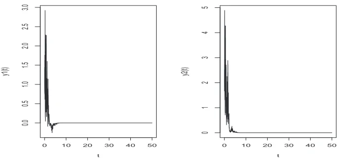
whereI₂ is the 2×2 identity matrix. It is therefore easy to see that the linear SDE (5.1) is almost surely exponentially stable if and only ifa <0.5(σ₁2−σ₂2). By Theorem 4.4, we can then conclude that the stochastic theta method applied to the SDE (5.1) is almost surely exponentially stable for all sufficiently small step sizes, which is one of the key results of [4]. Figure 1 shows a computer simulation of the paths ofy₁(t) andy₂(t) using the stochastic theta method with the parameterθ= 0.5 and the step size Δt= 0.001 and the system parametersa= 1,σ₁= 2,σ₂= 1 as well as the initial valuesy₁(0) = 1,y₂(0) = 2. The computer simulation clearly supports our theoretical result.

0 10 20 30 40 50

0.0

0.5

1.0

1.5

2.0

2.5

3.0

t

y1(t)

0 10 20 30 40 50

012345

t

y2(t)

Fig. 1_{.The sample paths of the solution to the SDE (5.1).}

Example 5.2. _{Consider the two-dimensional stochastic differential equation}

dy(t) =f(y(t))dt+Gy(t)dw₁(t) (5.3)

ont≥0 with initial valuey(0) =y₀∈R2,

f(y) =

2y₂cosy₁+ siny₁

−y₁+ siny₂

, G=

3 −0.3

−0.3 3

.

LetV(y, t) =|y|2. It is easy to verify that

LV(y, t) = 2y₁(2y₂cosy₁+ siny₁) + 2y₂(−y₁+ siny₂) +|Gy|2≤13.89|x|2

and

|V_x(x, t)Gx|2 =|2xTGx|2≥29.16|x|4.

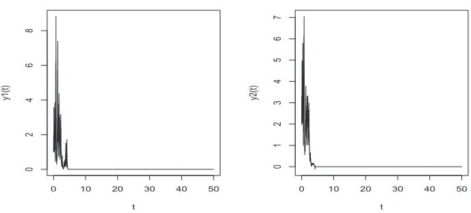
By Theorem 4.5, the SDE (5.3) is almost surely exponentially stable, while by Theo-rem 4.7, the stochastic theta method applied to the SDE is also almost surely expo-nentially stable for all sufficiently small step sizes. Figure 2 is the computer simulation of the paths ofy₁(t) andy₂(t) using the Euler–Maruyama method (i.e., the stochastic theta method with the parameterθ= 0) and the step size Δt= 0.001 as well as the initial values y₁(0) = 1,y₂(0) = 2. Again, the computer simulation clearly supports our theoretical result.

6. Conclusions. In this paper, we have shown that, under the standing As-sumption 2.1,

(A)⇐(B)⇔(C)⇒(D),

where

(A) denotes the almost sure exponential stability of the SDE,

(B) denotes thepth moment exponential stability of the SDE (p∈(0,1) is suffi-ciently small),

0 10 20 30 40 50

0

2

4

6

8

t

y1(t)

0 10 20 30 40 50

0

1

2

3

4

5

6

7

t

y2(t)

Fig. 2_{.The sample paths of the solution to the SDE (5.3).}

(C) denotes thepth moment exponential stability of the stochastic theta method for a sufficiently small step size,

(D) denotes the almost sure exponential stability of the stochastic theta method for a sufficiently small step size.

In particular, our new theory enables us to study the almost sure exponential stability of SDEs using the stochastic theta method, instead of the method of the Lyapunov functions. That is, we can now carry out careful numerical simulations using the stochastic theta method with a sufficiently small step size Δt. If the stochastic theta method ispth moment exponentially stable for a sufficiently smallp∈(0,1), we can then infer that the underlying SDE is almost surely exponentially stable.

Our new theory also enables us to show the ability of the stochastic theta method to reproduce the almost sure exponential stability of the SDEs. In the case when the underlying SDE is linear (namely, (4.3)), recalling the classical result (A)⇔(B) established by Arnold, Kliemann, and Oeljeklaus [2], we have shown (A) ⇒ (D). That is, we have obtained the positive answer to problem (P1). In the case when the underlying SDE is nonlinear, we know that (A) does not imply (B) in general. However, we have recalled one of the most useful criteria, Theorem 4.5, for almost sure exponential stability and shown that the SDE ispth moment exponentially stable for all sufficiently smallpunder the same conditions. Consequently, we have obtained a positive answer to problem (P2).

REFERENCES

[1] L. Arnold,Stochastic Differential Equations: Theory and Applications, Wiley, 1972.

[2] L. Arnold, W. Kliemann, and E. Oeljeklaus_{, Lyapunov exponents of linear stochastic} systems, in Lyapunov Exponents, Lecture Notes in Math. 1186, Springer, New York, 1986, pp. 85–125.

[3] C. T. H. B. Baker and E. Buckwar,Exponential Stability inp-th Mean of Solutions, and of Convergent Euler-Type Solutions, to Stochastic Delay Differential Equations, Numer. Anal. Report 390, University of Manchester, 2001.

[4] G. Berkolaiko, E. Buckwar, C. Kelly, and A. Rodkina_{,Almost sure asymptotic} stabil-ity analysis of the Euler-Maruyama method applied to a test system with stabilising and destabilising stochastic perturbations, LMS J. Comput. Math., 15 (2012), pp. 71–83.

[5] E. Buckwar and C. Kelly_{,Towards a systematic linear stability analysis of numerical} meth-ods for systems of stochastic differential equations, SIAM J. Numer. Anal., 48 (2010), pp. 298–321.

[6] A. Friedman_{,Stochastic Differential Equations and Their Applications, Academic Press, New}

York, 1976.

[7] D. J. Higham_{,Mean-square and asymptotic stability of the stochastic theta method, SIAM J.}

Numer. Anal., 38 (2000), pp. 753–769.

[8] D. J. Higham, X. Mao, and A. M. Stuart_{,Strong convergence of Euler-type methods for} nonlinear stochastic differential equations, SIAM J. Numer. Anal., 40 (2002), pp. 1041– 1063.

[9] D. J. Higham, X. Mao, and A. M. Stuart_{,Exponential mean-square stability of numerical} solutions to stochastic differential equations, LMS J. Comput. Math., 6 (2003), pp. 297– 313.

[10] D. J. Higham, X. Mao, and C. Yuan_{,Almost sure and moment exponential stability in the} numerical simulation of stochastic differential equations, SIAM J. Numer. Anal., 45 (2007), pp. 592–609.

[11] R. Z. Khasminskii, Stochastic Stability of Differential Equations, Sijthoff and Noordhoff,

Alphen aan den Rijn, 1981.

[12] P. E. Kloeden and E. Platen_{, Numerical Solution of Stochastic Differential Equations,}

Springer-Verlag, New York, 1992.

[13] G. S. Ladde and V. Lakshmikantham_{,Random Differential Inequalities, Academic Press,}

New York, 1980.

[14] X. Mao_,Stability of Stochastic Differential Equations with Respect to Semimartingales_,

Long-man Scientific and Technical, Harlow, UK, 1991.

[15] X. Mao_{,Exponential Stability of Stochastic Differential Equations, Marcel Dekker, New York,}

1994.

[16] X. Mao,Stochastic Differential Equations and Applications, Horwood, Chichester, UK, 1997.

[17] X. Mao, Y. Shen, and A. Gray_{, Almost sure exponential stability of backward} Euler-Maruyama discretizations for hybrid stochastic differential equations, J. Comput. Appl. Math., 235 (2011), pp. 1213–1226.

[18] X. Mao and C. Yuan_{,Stochastic Differential Equations with Markovian Switching, Imperial}

College Press, London, 2006.

[19] S. Pang, F. Deng, and X. Mao_{,Almost sure and moment exponential stability of Euler–} Maruyama discretizations for hybrid stochastic differential equations, J. Comput. Appl. Math., 213 (2008), pp. 127–141.

[20] Y. Saito and T. Mitsui_{,Stability analysis of numerical schemes for stochastic differential} equations, SIAM J. Numer. Anal., 33 (1996), pp. 2254–2267.

[21] H. Schurz,Stability, Stationarity, and Boundedness of some Implicit Numerical Methods for Stochastic Differential Equations and Applications, Ph.D. thesis, Logos Verlag, Berlin, 1997.

[22] D. R. Smart_{,Fixed Point Theorems, Cambridge University Press, Cambridge, UK, 1974.}

[23] A. M. Stuart and A. R. Humphries_{,Dynamical Systems and Numerical Analysis, Cambridge}

University Press, Cambridge, UK, 1996.

[24] D. Talay_{,Approximation of the invariant probability measure of stochastic Hamiltonian} dissi-pative systems with non globally Lipschitz co-efficients, in Progress in Stochastic Structural Dynamics, Volume 152, R. Bouc and C. Soize, eds., Publication du L.M.A.-CNRS, 1999. [25] F. Wu, X. Mao, and L. Szpruch_{,Almost sure exponential stability of numerical solutions for}

SDDEs, Numer. Math., 115 (2010), pp. 681–697.

[26] F. Wu, X. Mao, and P. Kloeden_{,Almost sure exponential stability of the Euler–Maruyama} approximations for stochastic functional differential equations, Random Oper. Stochastic Equations, 19 (2011), pp. 105–216.

[27] F. Wu, X. Mao, and P. Kloeden_{,Discrete Razumikhin-type technique and stability of the} Euler–Maruyama method to stochastic functional differential equations, Discrete Contin. Dyn. Syst., 33 (2013), pp. 885–903.