Estimating Residual Faults from Code Coverage

City, University of London Institutional Repository

Citation

:

Bishop, P. G. (2002). Estimating Residual Faults from Code Coverage. Paper

presented at the SAFECOMP 2002, 10 - 13 Sept 2002, Catania, Italy.

This is the unspecified version of the paper.

This version of the publication may differ from the final published

version.

Permanent repository link:

http://openaccess.city.ac.uk/547/

Link to published version

:

Copyright and reuse:

City Research Online aims to make research

outputs of City, University of London available to a wider audience.

Copyright and Moral Rights remain with the author(s) and/or copyright

holders. URLs from City Research Online may be freely distributed and

linked to.

City Research Online:

http://openaccess.city.ac.uk/

[email protected]

Estimating Residual Faults from Code Coverage

Peter G Bishop

Adelard and Centre for Software Reliability City University

Northampton Square London EC1V 0HB, UK

[email protected], [email protected]

Abstract. Many reliability prediction techniques require an estimate for the number of residual faults. In this paper, a new theory is developed for using test coverage to estimate the number of residual faults. This theory is applied to a specific example with known faults and the results agree well with the theory. The theory is used to justify the use of linear extrapolation to estimate residual faults. It is also shown that it is important to establish the amount of unreachable code in order to make a realistic residual fault estimate.

1 Introduction

Many reliability prediction techniques require an estimate for the number of residual faults [2]. There are a number of different methods of achieving this; one approach is to use the size of the program combined with an estimate for the fault density [3]. The fault density measure might be based on generic values, or past experience, including models of the software development process [1,7].

An interesting alternative approach was suggested by Malaiya, Denton and Li [4,5] who showed that the growth in the number of faults detected was almost linearly correlated with the growth in coverage. This was illustrated by an analysis of the coverage data from an earlier experiment performed on the PREPRO program by Pasquini, Crespo and Matrella [6].

This paper develops a general theory for relating code coverage to detected faults that differs from the one developed in [4]. The results of applying this model are presented, and used to justify a simple linear extrapolation method for estimating residual faults.

2 Coverage growth theory

We have developed a coverage growth model that uses different modelling assumptions from those in [4]. The assumptions in our model are that:

• there is a fixed execution rate distribution for the segments of code in the program (for a given input profile)

• there is a fixed probability of failure per execution rate, f

The full theory is presented in the Appendix, but the general result is that:

)

(

)

(

t

N

C

f

t

M

=

⋅

⋅

where the following definitions are used:

N0 initial number of faults

N(t) residual faults at time t

M(t) detected faults at time t, i.e. N0 – N(t)

C(f⋅t) fraction of covered code at time f⋅t

f probability of failure per execution of the faulty code

Note that this theory should work with any coverage measure; a fine-grained measure like MCDC coverage should have a higher value of f than a coarser measure like statement coverage. Hence a measure with a larger f value will detect the same number of faults at a lower coverage value.

With this theory, the increase in detected faults M is always linear with increase in coverage C if f = 1. This is true even if the coverage growth curve against time is non-linear (e.g. an exponential rise curve) because the fault detection curve will mirror the coverage growth curve; as a result, a linear relationship is maintained between M and C.

If f < 1, a non-linear coverage growth curve will lead to a non-linear relationship between M and C. In the Appendix one particular growth model is analysed where the coverage changes as some inverse power of the number of tests T, i.e. where:

p

kT

t

C

+

=

−

1

1

)

(

1

Note that 1 − C(t) is equivalent to the proportion of uncovered code, U(t)this was used in the Appendix as it was mathematically more convenient. With this growth curve, the Appendix shows that the relationship between detected faults M and coverage C is:

)

1

)(

1

(

)

1

(

1

0

f

C

f

C

N

M

−

−

+

−

−

=

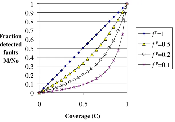
The normalised growth curves of detected faults M / N0 versus covered code C

from equation (3) are shown in the figure below for different values of fp

0

0.1

0.2

0.3

0.4

0.5

0.6

0.7

0.8

0.9

1

0

0.5

1

Coverage (C)

Fraction

detected

faults

M/No

f

₌₁

f

_=0.5

f

_=0.2

f

_=0.1

Fig. 1. Normalised graph of faults detected versus coverage (inverse power coverage growth)

Analysis of equation (2) shows that the slope approximates to f p

at U = 1, while the final slope is 1/ f p

at U = 0, so if for example f p

= 0.1then the initial slope is 0.1 and the final slope is 10. This would mean that the relationship between N and U is far from linear (i.e. the initial and final slopes differ by a factor of 100).

If the value of p is small (i.e. growth in coverage against tests has a “long tail”) this reduces the effect of having a low value for f as is illustrated in the table below.

Table 1. Example values of f p

f p

f p=1 p=0.5 p=0.1

1.0 1.0 1.0 1.0

0.5 0.5 0.71 0.93

0.1 0.1 0.42 0.79

This suggests that non-linearity can be reduced and hence permit more accurate predictions of the number of residual faults.

To evaluate the theory, the assumptions and its predictions in more detail, we applied the model to the PREPRO program.

3 Evaluation of the theory on the PREPRO example

containing a specification for the antenna. The antenna description is parsed by the program and, if the specification is valid, a set of antenna parameters computed and sent to the standard output. The program has to detect violations of the specification syntax and invalid numerical values for the antenna. This program is quite complex, containing 7555 executable lines of code.

The original experiment did not provide the data necessary to evaluate our model so we obtained a copy of the program and supporting test harness from the original experimenters [6], so that additional experiments could be performed, namely the measurement of:

• the growth in coverage of executable lines, C(t) • the mean growth in detected faults, M(t)

• the probability of failure of per execution of a faulty line, f

3.1 Measurement of growth in line coverage

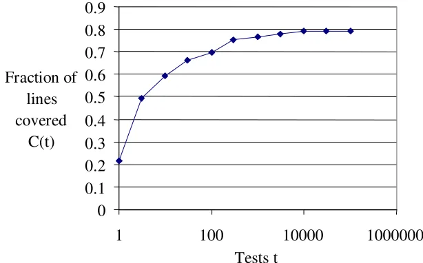
In our proposed model, we assumed that there was an equal chance of a fault being present in any executable line of code. We therefore needed to measure the growth in line coverage against tests (as this was not measured in the original experiment). The PREPRO software was instrumented using the Solaris statement coverage tool tcov, and statement coverage was measured after different numbers of tests had been performed. The growth line coverage against time is shown below.

0

0.1

0.2

0.3

0.4

0.5

0.6

0.7

0.8

0.9

1

100

10000

1000000

Tests t

Fraction of

lines

covered

C(t)

Fig. 2. Coverage growth for PREPRO (line coverage).

It can be seen that around 20% (1563 out of 7555) of executable lines are uncovered even after a large number of tests.

Table 2. Analysis of uncovered code blocks

Entry condition to block Number

of blocks Numberof lines

Uncallable (“dangling” function) 1 6

Internal error (e.g. insufficient space in internal table

or string, or malloc memory allocation problem) 47 248 Unused constructs, detection of invalid syntax 231 1309

Total 279 1563

The first type of uncovered code is definitely unreachable. The second is probably unreachable because the code detecting internal errors cannot be activated as this would require changes to the code to reduce table sizes, field sizes, etc. The final class of uncovered code is potentially reachable given an alternative test harness that covered the description syntax more fully and also breaks the syntax rules.

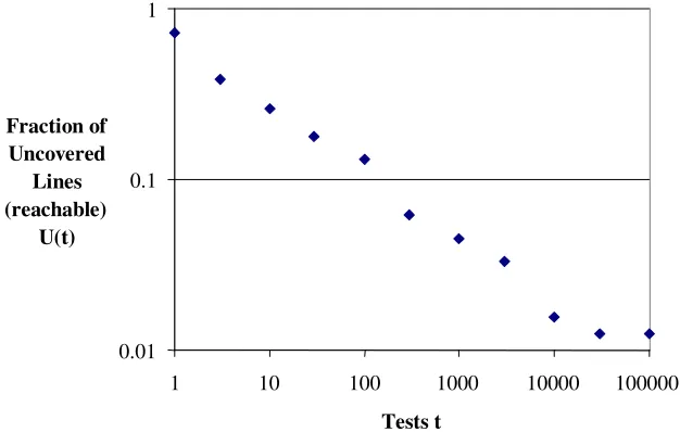
The “asymptote” observed in Fig.3 of 1563 uncovered lines is assumed to represent unreachable code under the test profile generated by the harness. This stable value was achieved after 10 000 tests and was unchanged after 100 000 tests. If we just consider the 5992 lines that are likely to be reachable with the test profile we get the following relationship between uncovered code and the number of tests.

0.01 0.1 1

1 10 100 1000 10000 100000

Tests t Fraction of

Uncovered Lines (reachable)

U(t)

Fig. 3. Uncovered lines (excluding unreachable code) vs. tests (log-log graph)

3.2 Measurement of the mean growth in detected faults

The fault detection times will vary with the specific test values chosen. To establish the mean growth in detected faults, we measured the failure rate of each fault inserted individually into PREPRO, using a test harness where the outputs of the “bugged” version were compared against the final version. This led to an estimate for the failure probability per test, λi of each fault under the given test profile. These probabilities

were used to calculate the mean number of faults detected after a given number of tests using the following equation:

∑

−

−

=

1

exp(

)

)

(

t

t

M

λ

where t is the number of tests. This equation implies that several faults could potentially be detected per test—especially during the early test stages when the faults detected have failure probabilities close to unity. In practice, several successive tests might be needed to remove a set of high probability faults. This probably happened in the original PREPRO experiment where 9 different faults caused observable failures in the first 9 tests.

We observed that 4 of the 33 faults documented within the code did not appear to result in any differences compared to the “oracle”. These faults were pointer-related and for the given computer, operating system and compiler, the faulty assignments might not have had an effect (e.g. if temporary variables are automatically set to zero, this may be the desired initial value, or if pointers are null, assignment does not overwrite any program data). The mean growth in detected faults, M(t), is shown below.

0 5 10 15 20 25 30 35

1 10 100 1000 10000 100000

Mean faults detected M(t)

Tests

3.3 Measurement of segment failure probability f

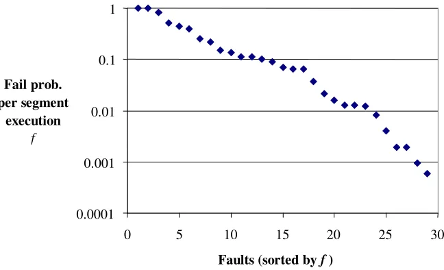
In the theory it is assumed that f is a constant. To evaluate this we measured the number of failures for each of the known faults (activated individually) under extended testing. Using the statement coverage tool, tcov, we also measured the associated number of executions of the faulty line. Taking the ratio of these two values we computed the failure probability per execution of the line f. It was found that f was not constant for all faults, the distribution is shown in the figure below.

0.0001 0.001 0.01 0.1 1

0 5 10 15 20 25 30

Faults (sorted by f ) Fail prob.

per segment execution

f

Fig. 5. Distribution of segment failure probabilities

There is clearly a wide distribution of values of f, so to apply the theory we should know the failure rates of individual faults (or the likely distribution of f). However we know that the range of values for f p

is more restricted than f. We can also take the geometric mean of the individual f values to ensure that all values are given equal weight, i.e. fmean = (Π fi)

1/Nf _{where N}

f is the number of terms in the product. The

geometric mean of the values was found to be fmean = 0.0475.

4 Comparison of the theory with actual faults detected

The estimated fault detection curve, M(t), based on known fault failure probabilities, can be compared with the growth predicted using equation (3) using the values of f and p derived earlier. The earlier analysis gave the following model parameters:

f = 0.0475 p = 0.40 So the value for f p

is: f p

= 0.0475 0.4

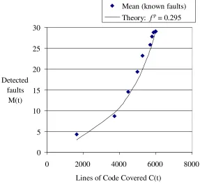
The comparison of the actual and predicted growth curves is shown in figure 6 below. Note that the theoretical curve is normalised so that 5992 lines covered is viewed as equivalent to C=1 (as this is the asymptotic value under the test conditions).

Mean (known faults)

Theory:

f

_{= 0.295}

0

5

10

15

20

25

30

0

2000

4000

6000

8000

Lines of Code Covered C(t)

Detected

faults

M(t)

Fig. 6. Faults detected versus coverage (theory and actual faults)

It can be seen that the theory prediction and mean number detected (based on the failure rates of actual faults) are in reasonable agreement.

5 Estimate of residual faults

The coverage data obtained for PREPRO are shown below:

Table 3. Coverage achieved and faults detected. Total executable lines 7555 Covered after test 100 000 5992

Unreachable 254

Potentially reachable 1309

Taking account of unreachable code, the final fraction of uncovered code is: C = 5992 / (7555-254) = 0.785

If we used equation (3) and took C=0.785 and f p

= 0.295, we would obtain a prediction that the fraction of faults detected is 0.505. However this would be a misuse of the model, as the curve in figure 6 is normalised so that 5992 lines is regarded as equivalent to C=1.

Using the model to extrapolate backwards from C=1, only one fault would be undetected if the coverage was 0.99 (5932 lines covered out of 5992). As this level of coverage was achieved in less than 10 000 tests and 100 000 tests were performed in total, it is reasonable to assume that a high proportion of the faults have been detected for the 5992 lines covered.

The theory shows that there can be a non-linear relationship between detected faults and coverage, even if there is an equal probability of a fault in each statement. Indeed, given the measured values of f and p, good agreement is achieved using an assumption of constant fault density. Given a constant fault density and a high probability that faults are detected in the covered code, we estimate the density of faults in the covered code to be:

29/5992

= 0.0048 faults/line

and hence the number of faults in uncovered code is: N = 1563 ⋅ 0.0048

= 7.5

or if we exclude code that is likely to be always unreachable: N = 6.3

So from the proportion of uncovered code, the estimate for residual faults lies between 6 and 8. The known number of undetected faults for PREPRO is 5, so the prediction is close to the known value.

6 Discussion

The full coverage growth theory is quite complex, but is does explain the shape of the fault-coverage growth curves observed in [4,5] and our evaluation experiment. Clearly there are difficulties in applying the full theory. We could obtain a coverage versus time curve directly (rather than using p), but there is no easy way of obtaining f. In addition we have a distribution of f values rather than a constant, which is even more difficult to determine.

However our analysis indicates that the use of the full model is not normally necessary. While we have only looked at one type of coverage growth curve, the theory suggests that any slow growth curve would reveal a very high proportion of the faults in the code covered by the tests. It could therefore be argued that the number of residual faults is simply proportional to the fraction of uncovered code (given slow coverage growth).

Ideally, the fault prediction we have made should be assessed by testing the uncovered code. This would require the involvement of the original authors, which is impractical as development halted nearly a decade ago. Nevertheless, the fault density values are consistent with those observed in other software, and deriving the expected faults from a fault density estimate is a well-known approach [1,3,7]. The only difference here is that we are using coverage information to determine density for covered code, rather than treating the program as a “black box”.

Clearly, there are limitations in this method (such as unreachable code), which might result in an over-estimate of N, but this would still be a useful input to reliability prediction methods [2].

7 Conclusions

1. A new theory has been presented that relates coverage growth to residual faults.

2. Application of the theory to a specific example suggests that simple linear extrapolation of code coverage can be used to estimate the number of residual faults.

3. The estimate of residual faults can be reduced if some code is unreachable, but it is conservative to assume that all executable code is reachable.

4. The method needs to be evaluated on realistic software to establish what level of accuracy can be achieved in practice.

8 Acknowledgements

This work was funded by the UK (Nuclear) Industrial Management Committee (IMC) Nuclear Safety Research Programme under British Energy Generation UK contract PP/114163/HN with contributions from British Nuclear Fuels plc, British Energy Ltd and British Energy Group UK Ltd. The paper reporting the research was produced under the EPSRC research interdisciplinary programme on dependability (DIRC).

References

1 R.E. Bloomfield, A.S.L. Guerra, "Process Modelling to Support Dependability Arguments", DSN 2002 Washington, DC, 23-26 June, 2002

2 W. Farr. Handbook of Software Reliability Engineering, M. R. Lyu, Editor, chapter Software Reliability Modeling Survey, pages 71--117. McGraw-Hill, New York, NY, 1996 3 M. Lipow, "Number of Faults per Line of Code," IEEE Trans. on Software Engineering,

SE-8(4):437-439, July 1982.

4 Y. K. Malaiya and J. Denton, “Estimating the number of residual defects”, HASE’98, 3rd

IEEE Int’l High-Assurance Systems Engineering Symposium, Maryland, USA, November

5 Y.K. Malaiya, J. Denton and M.N. Li., Estimating the number of defects: a simple and intuitive approach, Proceedings of the Ninth International Symposium on Software Reliability Engineering, Paderborn, Germany, November 4-7, 1998, pp. 307-315

6 A. Pasquini, A. N. Crespo and P. Matrella, “Sensitivity of reliability growth models to operational profile errors”, IEEE Trans. Reliability, vol. 45, no. 4, pp 531–540, Dec. 1996 7 K. Yasuda, “Software Quality Assurance Activities in Japan”, Japanese Perspectives in

Software Engineering, 187-205, Addison-Wesley, 1989

Appendix: Coverage growth theory

In this analysis of coverage growth theory, the following definitions will be used: N0 initial number of faults

N(t) residual faults at time t

M(t) detected faults at time t, i.e. N0 – N(t)

C(t) fraction of covered code at time t U(t) fraction of uncovered code, i.e. 1 – C(t) Q execution rate of a line of executable code

f probability of failure given execution of fault in line of code

We assume the faults are evenly distributed over all lines of code. If we also assume there is a constant probability of failure f per execution of an erroneous line, then the mean number of faults remaining at time t is:

∫

_⋅

=

0

0

(

)

)

(

t

N

pdf

Q

e

dQ

N

Similarly the uncovered lines remaining at time t are:

∫

_⋅

=

0

(

)

)

(

t

pdf

Q

e

dQ

U

The equations are very similar, apart from the exponential term. Hence we can say by simple substitution

)

(

)

(

t

N

U

f

t

N

=

⋅

⋅

Substituting N(t) = N0 – M(t), and U(t) = 1 – C(t) and rearranging we obtain:

)

(

)

(

t

N

C

f

t

M

=

⋅

⋅

So when f=1, we get linear growth of faults detected, M, versus coverage, C, regardless of the distribution of execution rates, pdf(Q).

Inverse power law coverage growth

Let us take an example of slow coverage growth, where the uncovered code is some inverse power of t:

p

kt

t

U

+

=

1

1

)

(

where p < 1. Rearranging we obtain:

p

kU

U

t

1

1

_









 −

=

(10)

Substituting for t in equation (7), it can be shown that:

)

1

(

0

f

U

f

U

N

N

−

+

=

For the case where U << f:p

U

N

N

_≈

0

f

(12)

So the limiting value to the gradient is:

p

f

N

dU

dN

_{→ −}

as

U

→

0

(13)