E. R. Echevarria1,2,3 , M. A. Hemer1, and N. J. Holbrook2,3
1CSIRO Oceans and Atmosphere, Hobart, Tasmania, Australia,2Institute for Marine and Antarctic Studies, University of
Tasmania, Hobart, Tasmania, Australia,3Australian Research Council Centre of Excellence for Climate Extremes,
University of Tasmania, Hobart, Tasmania, Australia
Abstract
Our understanding of the seasonal variability in the global wind wavefield is revisited here using a novel analysis that resolves the directional wave spectra. Empirical orthogonal function analysis was applied to modeled wave spectral data from a WAVEWATCH III hindcast across a sparse global grid to identify the main patterns of the climatological wave spectral variability at each grid point. Prior methods have focused on the variability of two modes of the wavefield—locally generated sea and the primary swell component. Our results also consider additional wave modes at each location, enabling us to track the passage of the less dominant swell modes. Consistent with existing climatological knowledge, the main modes of wave spectral variability at high latitudes are related to eastward propagating waves that disperse equatorward as swell following great circle paths. However, despite being the less energetic mode, the Northern Hemisphere generated swell is found to propagate into the Southern Hemisphere further than the more energetic Southern Hemisphere swell which propagates northward. In the equatorial zone, a complex multimodal wave climate is found, with the spectra variability modulated by remotely generated swell and higher‐frequency waves associated with the prevailing winds. The evolution of these patterns throughout the year is clearly depicted. Overall, our approach captures a more complete picture of the seasonal variability of the global wavefield, by accounting for all the wave modes observed in the spectra at each location together with their temporal variability.Plain Language Summary
Waves generated by the wind blowing over the surface of the ocean are able to travel immense distances and reach distant coasts (e.g., it has been recognized since the 1950s that the coasts of California receive waves generated in the Southern Ocean). This means that the wave climate of a given region can be very complex, having waves generated by local winds but also from many remote places at once (multiple swellfields). In this study, we present a new method to examine seasonal variations in the global wave climate which accounts for the full directional wave spectra and includes wave systems with different frequencies and directions separately, as opposed to using integrated waveparameters, such as significant wave height or mean direction. Our results show how low‐frequency swell waves propagate across ocean basins from high to low latitudes of both hemispheres, higher‐frequency waves that are a product of the local winds, and the variation in the intensity of these signals throughout the year. We believe future wave studies can benefit from this approach, since a concise and yet more complete representation of the wave climate variability can be achieved.
1. Introduction
Wind‐generated waves play a critical role in processes such as: alongshore sediment transport, which can translate into changes in the coastline position (Dean & Dalrymple, 2004); the Stokes drift (Longuet‐ Higgins, 1953) which is a very important consideration for search and rescue activities; exchanges of heat, mass, and momentum with the atmosphere (Cavaleri et al., 2012); and extreme coastal sea level assessments (Vitousek et al., 2017). Importantly, engineering projects such as the construction of coastal structures, offshore activities, or the planning of shipping routes require accurate predictions of the wind wave climate. Wave observations from moored buoys, although highly accurate, usually span short periods of time and are sparsely distributed around the world, not being appropriate for global studies.
Understanding the global characteristics of wind waves and their variability is indispensable. During recent decades, the development of numerical wave models and advent of satellite remote sensing systems have made it possible to undertake global wind wave studies, which have brought about a deeper ©2019. American Geophysical Union.
All Rights Reserved. Key Points:
• Dominant modes of seasonal variability in global directional wind wave spectra were identified
• The wave climate at middle to high latitudes is well described with one or two wave modes, but in the tropics three to four modes are needed
• The rotation of the wave signals at high latitudes was captured, which could be beneficial for future studies
Supporting Information:
•Supporting Information S1
Correspondence to: E. R. Echevarria, [email protected]
Citation:
Echevarria, E. R., Hemer, M. A., & Holbrook, N. J. (2019). Seasonal variability of the global spectral wind wave climate.Journal of Geophysical Research: Oceans,124, 2924–2939. https://doi.org/10.1029/2018JC014620
Received 2 OCT 2018 Accepted 3 APR 2019
understanding of wave propagation and interconnections between ocean basins. For example, Young (1999) studied the seasonal variability of the global wave climate using altimeter‐derived and modeled data. He observed that the highest wave conditions are attained at high latitudes, with the Northern Hemisphere (NH) presenting a higher seasonal variability than the Southern Hemisphere (SH). In addition, the Southern Ocean‐generated swell waves penetrate into the Indian, South Pacific, and South Atlantic Oceans and can even reach the NH during the austral winter (Snodgrass et al., 1966). In contrast, the seaso-nal variability in the equatorial regions is much less, with wave heights being much smaller year‐round. Sterl and Caires (2005), using 45 years of wave data from the European Centre for Medium‐Range Weather Forecasts Re‐Analysis‐40 reanalysis, concluded that the mean wave conditions are more intense in the Southern Ocean, but the most extreme wave heights are found in the North Atlantic, given that it has a lar-ger variability. Chen et al. (2002), using satellite altimeter‐derived wave data and scatterometer winds, and Semedo et al. (2011), using wave data from the European Centre for Medium‐Range Weather Forecasts Re‐ Analysis‐40 reanalysis, analyzed sea and swell waves separately. They both found that the wave climate in most areas of the world is dominated by swell and also defined a“swell front”as the area of separation of swell from the SH and NH, located in the equatorial region and varying seasonally, extending farther north (south) in austral winter (summer). In reality, however, no such“front”exists, with each swellfield continu-ing its propagation in its respective direction as a superimposed wavefield with multiple swell modes.
Typically, studies of wind wave variability across different time scales have been performed with integrated parameters (such as significant wave height, peak period, or mean direction with, at best, sea and swell dis-tinguished). These parameters arise from a statistical description of the wave record and are widely used in both scientific and industrial applications. However, there are occasions in which the integrated parameters cannot properly describe the wave climate of a particular region, given that some characteristics of the wave spectrum are poorly resolved or not resolved at all. For example, Villas Bôas et al. (2017) studied the seasonal variability of the wave climate off the California coast and observed that the wave spectrum can be separated by up to seven different partitions, each one having characteristic frequencies and directions. Moreover, no clear predominance of any of these modes throughout the year was observed, as all displayed a strong sea-sonal variability. Portilla‐Yandún et al. (2016), using wave spectral data in the eastern equatorial Pacific, identified four distinctive wave systems. These studies illustrate the complexity that is often observed in the multimodal wave climate, which cannot be properly captured with integrated parameters alone. Instead, the most complete depiction of surface ocean waves is given by the directional wave spectrum, which describes how wave spectral density is distributed over frequencies and directions and allows us to identify the different wave modes.
Increasingly, the potential contributions of waves to coastal and ocean challenges are being identified (e.g., coastal sea level, Arns et al., 2017; Vitousek et al., 2017; and ocean mixing, D'Asaro et al., 2014; Van Roekel et al., 2012). The total wave energy (as represented by integrated parameters) is likely a poor representation of the potential contribution of a multimodal sea to these processes, with different modes of the wavefield, of different frequency or direction, likely leading to alternate response(s). For example, coastal sea level will be dependent only on the modes of the wavefield with a shoreward propagating component and more heavily biased by low‐frequency modes. This motivates us to adopt a different approach from that used so far in wind wave studies. The aim of this research is to assess the seasonal variability of the directional wave spectra at the global scale. In order to accomplish this, given the sparsity of wave spectral measurements across the world, we have used data from a validated global wave hindcast.
This paper is organized as follows: Section 2 provides a description of the wave data utilized and the meth-odology employed to extract the main modes of spectral variability, section 3 compares observed and mod-eled directional wave spectra and discusses the potential errors in the spectral information used, section 4 presents the main results of this analysis, andfinally these results are discussed in some detail in section 5.
2. Data and Methods
2.1. The CAWCR Wave Hindcast
implementation of the WAVEWATCH III model version 4.08 (Tolman, 2009). The Climate Forecast System Reanalysis 10‐m winds and sea ice concentration data (Saha et al., 2010) were used to force the simulations. Some of the most relevant features of the hindcast configuration include the Ardhuin et al. (2010) source term parametrizations, specifically configured for utilization with the Climate Forecast System Reanalysis winds; the Discrete Interaction Approximation (Hasselmann et al., 1985) for nonlinear wave–wave inter-actions; and the third‐order Ultimate Quickest propagation scheme (Leonard, 1979; Leonard, 1991), including the garden sprinkler effect correction (Tolman, 2002), Joint North Sea Wave Project bottom fric-tion, and Battjes and Janssen (1978) shallow water depth breaking. Besides, an increase of the sheltering term from 1.0 to 1.2 (related to an effective wind reduction by shorter waves) and decrease of the nondi-mensional growth factor of the input source term (βmax) from 1.52 to 1.33 were implemented (Durrant et al., 2014). WAVEWATCH III also accounts for wave energy blocking by obstacles that cannot be resolved by the model grid (Tolman, 2003). This is especially relevant in the Pacific region, where there is a significant number of small islands. Obstruction masks were computed using coastline information from the Global Self consistent Hierarchical High resolution Shoreline database. The model considers the varying sea ice concentrations, using the approach described by Tolman (2003); hence, there are high‐latitude grid points covered by ice during certain periods of the year, where no wave information is available. In order to ease the calculations, these grid points were not considered in this analysis. A thorough description of the model setup and configuration and its outputs and validation can be found in Durrant et al. (2014) and Hemer et al. (2017) and therefore is omitted here. However, we emphasize the fact that integrated parameters derived from the hindcast have been validated against observations and satellite data around the world, displaying a good performance of the model in terms of bias and root‐mean‐square error (RMSE) and suitability to perform accurate global wave climate estimations. Additionally, we include in this paper an assessment of the performance of the model to represent observed directional wave spectra.
2.2. EOF Analysis of Wave Spectra
The data selected for this study consist of hourly archives of variance spectral density from 1979 to 2016 (38 years) covering 312 grid cells across a sparsely distributed (10° resolution) global grid. These data are dis-tributed spectrally over frequencies ranging exponentially between 0.035 and 0.5 Hz (with 29 bins) and directions every 15° (24 bins). In thefirst instance, the objective was to study the main modes of seasonal variability of the wave spectra at particular locations. To accomplish this, an empirical orthogonal function (EOF) analysis was carried out. The EOF analysis, thoroughly described by Preisendorfer and Mobley (1988), is a commonly used technique in atmospheric and oceanographic sciences tofind spatial patterns of varia-bility of a certain variable and how they change through time (see, for instance, Gulev & Grigorieva, 2006; Hemer et al., 2010; Woolf et al., 2002 for wave‐related studies). In the present study, an EOF analysis was instead performed to obtain the patterns of variability of the wave spectral density in the frequency/direction domain at each location (which were related to different wave modes in the spectra), rather than geographical patterns of variability.
Focusing on one single location, the data have the formS(fi,θj,t) whereSis the waves' variance spectral
density, which is a function of frequencyfi, directionθj, and timet. Since this study aims to investigate
the seasonal variability of the wave spectra, the climatological monthly averages for the whole period (1979–2016) were computed, thus reducing the time dimension to 12. In this way, we consider the average monthly wave conditions. Hence, the components of the wave climate with higher temporal variability than the climatological scale are not analyzed here. The average of all months was subtracted from each of the monthly means in order to work with climatological monthly anomalies. Then, for every location and for everyt, the spectral density matrix was rearranged into a one‐dimensional array of dimension 696 (29 frequencies * 24 directions):
S fð 1;θ1;tÞ;S fð 1;θ2;tÞ;⋯;S fð 1;θ24;tÞ;S fð 2;θ1;tÞ;⋯;S fð 2;θ24;tÞ;⋯;S fð 29;θ1;tÞ;⋯;S fð 29;θ24;tÞ
M¼
S fð 1;θ1;t1Þ S fð 1;θ1;t2Þ … S fð 1;θ1;t12Þ S fð 1;θ2;t1Þ S fð 1;θ2;t2Þ … S fð 1;θ2;t12Þ
⋮ ⋮ ⋮
S fð 1;θ24;t1Þ S fð 1;θ24;t2Þ… S fð 1;θ24;t12Þ S fð 2;θ1;t1Þ S fð 2;θ1;t2Þ … S fð 2;θ1;t12Þ
⋮ ⋮ ⋮
S fð 2;θ24;t1Þ S fð 2;θ24;t2Þ … S fð 2;θ24;t12Þ
⋮ ⋮ ⋮
S fð 29;θ24;t1Þ S fð 29;θ24;t2Þ… S fð 29;θ24;t12Þ
2 6 6 6 6 6 6 6 6 6 6 6 6 6 6 6 6 6 4 3 7 7 7 7 7 7 7 7 7 7 7 7 7 7 7 7 7 5
The next step is to compute the covariance matrixF=MMT, and then the eigenvalue problemFC=CΛis solved. In this case,Λis a diagonal matrix containing the eigenvaluesλi, and the columns ofCare the
eigen-vectors!ci associated with the eigenvaluesλi. These eigenvectors are the EOFs or the principal patterns of
variability of the wave spectra, and the eigenvalues are a measure of the relative importance of those patterns (i.e., how much of the total variance they explain). The patterns obtained represent standing oscillations, and their evolution in time is depicted by the principal component (PC) time series, which are computed asM c!i.
Finally, the variance explained by theith EOF is calculated as (λi/∑λi) * 100. This analysis was repeated
individually for each of the 312 locations on the sparse global grid.
2.3. Spectral Data From NDBC Buoys
In order to assess the suitability of the hindcast directional wave spectra data used in this study, the monthly averaged modeled spectra were compared against observations. Unfortunately, measurements of directional wave spectra are very scarce and most are concentrated in the NH, particularly the United States. The National Oceanic and Atmospheric Administrations National Data Buoy Center (NDBC: www.noaa.ndbc. gov) maintains a network of buoys and coastal stations that measure oceanographic and atmospheric vari-ables, and directional wave spectra can be reconstructed for some of these buoys. The spectral reconstruction techniques depend on the system used to measure waves. In this case, the NDBC operates heave‐pitch‐roll buoys, single‐point systems that measure the sea surface elevation (heave) together with the E‐W and N‐S sea surface slopes (pitch and roll). The formulations for the wave spectra reconstruction are usually given in terms of cross‐spectral parameters C11(wave elevation spectral density), C22and C33(E‐W and N‐S wave slope spectral density), C23(cospectral density between E‐W and N‐S wave slopes), and Q12and Q13 (quad-rature spectral density between elevation and E‐W and N‐S slope time series, respectively). One of thefirst reconstruction methods was devised by Longuet‐Higgins et al. (1963), who approximated the directional wave spectra by a truncated directional Fourier series expansion. However, more recent methods of spectral reconstruction provide better directional resolution and have proven to be overall more realistic. One such method is the maximum entropy method. Here, we apply the maximum entropy method for reconstruction of observed directional spectra following the methods of Lygre and Krogstad (1986).
TheC11,r1,r2,θ1, andθ2values for six buoys were downloaded from the NDBC webpage, and the cross‐ spectral parameters were computed following Earle et al. (1999). Then, the hourly directional wave spectra for each one of the buoys was reconstructed using the set of equations described by Lygre and Krogstad (1986). The wave records from the buoys span different time ranges, and they all have several gaps and miss-ing values. Therefore, only data from the wave hindcast that coincided in time with data from the buoys were selected. Finally, the monthly averages for both the buoy and hindcast spectra were computed and compared.
3. Comparison Between Modeled and Observed Directional Wave Spectra
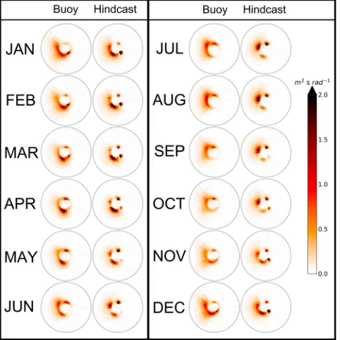
results are presented here for buoy 51028, which albeit not having the longest measurement record present characteristics of a multimodal wave climate that highlights the strength of the approach applied in this study. Figure 1 shows the monthly means of the directional wave spectra derived from the waves' hindcast and reconstructed from observations.
Qualitatively, the wave hindcast can be seen to reproduce the main wave modes present in the observations. There are two low‐frequency signals that are present all year round but with varying intensities: one directed to the NNE corresponding to the Southern Ocean generated swell which is more intense in the June–July–August (JJA) months and another one directed to the southeast that corresponds to North Pacific swell waves which are more intense in the December–January–February (DJF) months. There is also a higher‐frequency signal that shifts its direction through the year, being more southwesterly during DJF and more north-westerly in JJA, which is related to the equatorial trade winds. These char-acteristics can be observed both in the buoy and hindcast data. The hindcast tends to concentrate the wave energy in narrower signals (hence it attains larger values), whereas the mean spectra from the buoys present slightly broader signals.
The significant wave height (Hs) was computed from the directional
spec-tra as
Hsð Þ ¼t 4
ffiffiffiffiffiffiffiffiffiffiffiffiffiffiffiffiffiffiffiffiffiffiffiffiffiffiffiffiffiffiffiffiffiffiffiffiffiffiffiffiffiffi
1 NiNj∑i∑j
S fi;θj;t
s
(1)
whereNiis the number of frequencies,Njthe number of direction bins,
andSrepresents the wave spectra (i.e.,S(fi,θj,t) is the variance spectral
density at frequencyfi, directionθj, and timet).Hswas computed using
the directional spectra derived from the buoy and from the hindcast, and the correlation between theHstime
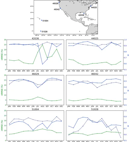
series for every month is shown in Figure 2.
In order to quantify the agreement between modeled and observed monthly mean wave spectra, two statis-tical parameters were considered: a normalized root‐mean‐square error (nRMSE) and the Pearson linear correlation coefficient (R). The nRMSE was computed as
nRMSE¼
ffiffiffiffiffiffiffiffiffiffiffiffiffiffiffiffiffiffiffiffiffiffiffiffiffiffiffiffiffiffiffiffiffiffiffiffiffiffiffiffiffiffiffiffiffiffiffiffiffiffiffiffiffiffiffiffiffiffiffiffiffiffiffiffiffiffiffiffiffiffiffiffiffiffiffiffiffiffiffiffiffiffiffiffi
1 NiNj∑i∑j
SBuoy fi;θj
−SHindcast fi;θj
2
s
*100=maxðSHindcastÞ (2)
whereSBuoyis the monthly mean wave spectrum reconstructed with the buoy data andSHindcastthe spec-trum derived from the hindcast. With the spectra discretized in 29 frequencies and 24 directions, nRMSE andRwere computed from a set of 696 data points for each spectrum. Figure 2 shows the nRMSE andR values for every month, for each of the buoys selected.
TheHstime series obtained from the hindcast and the observations are well correlated, withR> 0.8 for all
the selected buoys except 51028, where the correlation is high during the boreal summer but drops during winter. The RMSE values are within 10% of the maximum value attained by the model for all the selected buoys, except buoy 42036 (located in the Gulf of Mexico) where there are higher nRMSE from July to November, reaching a maximum of ~25%. This period is coincident with the Atlantic hurricane season (Landsea, 1993), and the relatively high errors are related to the inaccuracy of the wind forcing in resolving the cyclonic storms. If no normalization is applied to the RMSE calculation, a seasonal cycle of RMSE is obtained with higher values during the boreal winter and lower in summer, in agreement with results reported by Chawla et al. (2013). The monthly mean spectra from model and observations are well corre-lated, withR ~ 0.9 for buoys 44025, 46029, 46042, and 42036 (except from July to September for buoy 42036) andR~ 0.8 for buoys 51004 and 51028. In summary, the wave model makes a very good representa-tion ofHs(dotted line in Figure 2; also, see Durrant et al., 2014; Hemer et al., 2017), and of the monthly mean Figure 1.(left column) monthly mean spectra for buoy 51028 (0.0°N;
wave spectra, in the sense that it captures the wave modes present in the observed spectra and is well correlated with it. Therefore, with the data regarded suitable for this study, the methods described in section 2.2 were employed to investigate the seasonal variability of global directional wave spectra.
4. EOF Analysis Results
[image:6.612.90.522.91.564.2]The main modes of seasonal variability of the global directional wave spectra were computed following the method outlined in section 2.2. We recall that the reconstruction of the original spectral data from a few EOFs is achieved as follows:
Reconstructed spectra¼∑iEOFi*PCiþSmean (3)
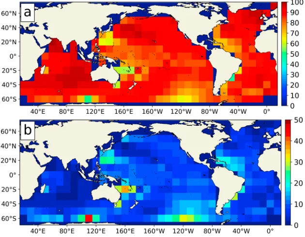
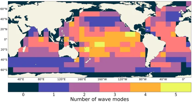
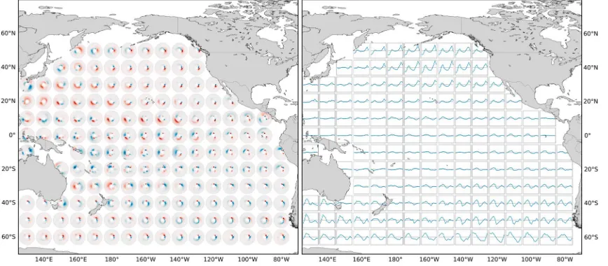
wherePCrepresents the PC time series,iis the number of EOFs selected, andSmeanthe average spectra for the whole period considered. Figure 3 shows the variance explained by thefirst two EOFs to show that they are sufficient to achieve an accurate data reconstruction; Figure 4 shows thefirst EOF patterns and Figure 5 their corresponding PC time series; Figure 6 shows the number of wave modes identified in the spectra at each location; Figure 7 presents the second EOF patterns and PC time series; andfinally, to complete the data reconstruction, the total average spectra are shown in Figure 8. Thus, together, thesefigures provide a comprehensive presentation of the seasonal variability of the global wave climate.
[image:7.612.217.532.92.337.2]First, in order to determine how many EOFs should be retained to adequately represent the seasonal varia-bility of the wave spectra, the variance explained by the first few EOFs was computed. The variance
Figure 3.Percentage of the total variance explained by the (a)first and (b) second empirical orthogonal function.
[image:7.612.178.574.513.682.2]explained by EOF‐1 is greater than 80% for the majority (~86%) of the grid cells (Figure 3). It attains very high values (>90%) in large areas of the Indian Ocean and at high latitudes of the North Pacific and North and southeast Atlantic. The minimum values are found east of Australia, south of Japan, in some regions of the Southern Ocean, and in the west part of the Atlantic. The variance explained by EOF‐2 in these regions is typically sufficient to combine with EOF‐1 to produce a total variance explained of >90%.
[image:8.612.176.575.90.258.2]There are a number of interesting features apparent in Figure 4. Since climatological monthly means were calculated from data over the period 1979–2016, our results correspond to a seasonal climatology of the wind wavefield. The main mode of seasonal variability at high latitudes in all ocean basins corresponds to low‐ frequency (~14 s) waves propagating eastward. These are swell waves generated by the intense westerlies in those regions, and EOF‐1 captures the variation in their intensity throughout the year. It can be seen that the South Pacific generated swell waves propagate to the north, reaching latitudes of ~20°N. This northern signal of the Southern Ocean generated swell has been long understood, following the founding work of Snodgrass et al. (1966). The swell signal follows a great circle track (path) shown with an orange line in Figure 4 (it is a curved line; however, this is not representative of a waves' rotation but an artifact of the geo-graphic projection used here). Furthermore, we see the directional widths of these signals are greater at high latitudes and become more focused in one direction as they propagate equatorward: In the vicinity of the storm tracks area, waves are being generated in an ample set of directions (mainly eastward), but in low lati-tudes far away from the generation area these waves arrive from one predominant direction and hence the
Figure 5.Principal component time series corresponding to thefirst empirical orthogonal function mode, from January to December. Units are meters squared second per radian.
[image:8.612.217.533.545.712.2]spectrum is narrower. A transition of the peak energy toward lower frequencies is observed between the high latitudes and the equatorial swell waves, evidencing their dispersive behavior.
Something analogous occurs with swell generated in the North Pacific and Atlantic, where the signals pagate to the south following a great circle route (green line in Figure 4). In this case, the swell waves pro-pagate further into the SH, reaching ~30°S latitude. The swell signals of the North and South Pacific have opposing signs, meaning when one increases the other decreases, and vice versa, evidencing the seasonal change in intensity of the westerlies in each hemisphere, which is greater in their respective winter. This southern extension of the NH generated swell is less well recognized in the literature, as it is typically domi-nated by the SH swell.
[image:9.612.92.526.92.282.2]In the equatorial regions, these two swell signals are present and their variability is captured by thefirst EOF. In the Pacific and Atlantic Ocean, EOF‐1 also shows the variability of higher‐frequency waves that propagate westward, generated by the prevailing trade winds. Besides, a strengthening of this signal is observed when moving from east to west in the equatorial region, consistent with the strengthening of the easterlies. These higher‐frequency signals can be decomposed into two parts: a negative signal, directed toward the north-west, which is in phase (same sign) with the Southern Ocean swell and has its maximum values at 10°S; and a positive one, directed to the southwest, in phase with the North Pacific swell with the maximum inten-sity at 10°N. These characteristics result from the variation of the equatorial easterly winds throughout the
Figure 7.(left panel) EOF‐2 patterns, shown for Pacific basin only. Axes limits as defined in Figure 4. (right panel) PC‐2 time series. Theyaxis for the PC ranges from−20 to 20, and the units are meter squared second per radian. EOF = empirical orthogonal function; PC = principal component.
year, which tend to be more northeasterly in DJF and more southeasterly in JJA. More regional features can also be appreciated, such as the shadowing influence of New Zealand (Laing, 2000), and the effect of south-erly winds blowing parallel to the Andes along the coast of Perú is observed in EOF‐1 as relatively high‐ frequency waves propagating northward. In the North Indian Ocean an intense high‐frequency signal is observed, related to the variability of the surface winds produced by the Asian Monsoon, which dominates the seasonal variability of the wave climate in this area. Again, the resolution of these regional features in our results exhibits the strength of the method to present a more complete picture of the seasonal variability of the global wave climate in a singlefigure.
These patterns are standing oscillations that represent the main modes of variability of the wave spectra, and it has been shown that they are associated with different wave modes in the spectrum. On the other hand, the PC time series (PCs) describe how these patterns (wave modes) evolve in time. The PCs corre-sponding to thefirst EOF for every location are shown in Figure 5. First, wefix all PCs to have a concave shape, with positive values in DJF and negative in JJA. This allows the EOF‐based method to present sea-sonal phase information consistently. For example, during DJF (boreal winter), the product of a positive PC value with the EOF patterns yields a positive anomaly in the NH and a negative anomaly in the SH (see equation (3)). As time progresses, the PC values become smaller, so that these anomalies (both posi-tive and negaposi-tive) lose their strength, until the PCs attain negaposi-tive values during midyear. At this stage, the SH patterns now represent a positive anomaly and the NH patterns a negative anomaly. The mini-mum (negative) values of the PCs are attained during the JJA months for almost every location, except in the South Pacific sector around 50°S. Here, the PCs are also negative during JJA, but the minimum negative values are attained during March–April–May (MAM) and September–October–November (SON) months, as a consequence of the two minima features associated with seasonal shifts of the SH storm belt. On the other hand, it can be observed that the grid cells with the lowest amplitude in their PCs (difference between maximum and minimum attained value) are located in the equatorial regions. This means that, in this area, the variability patterns depicted by the EOF remain relatively constant and with low values throughout the year. At high latitudes, the amplitude is greatly increased, meaning the EOF patterns present marked variability and oscillate with higher intensity in these areas. The largest amplitudes are found at high latitudes of the North Atlantic and Pacific Oceans and in the South Indian Ocean. The equatorial EOFs display much lower amplitude PCs.
To further support the assertion that the spectral patterns shown in EOF‐1 correspond to real wave modes in the spectra, a comparison with a complementary methodology was performed. Partitioned wave parameters from the CAWCR wave hindcast were used to identify the different wave systems in the spectra and compare them with those captured by EOF‐1. Four locations with distinctive spectral signatures were selected: in the Southern Ocean (180°E; 50°S), north Indian Ocean (90°E; 10°S), equatorial eastern Pacific (100°W; 0°), and in the north Atlantic (30°W; 40°N). The significant wave height, peak frequency, and peak direction of the
first four partitions were mapped onto a frequency/direction grid using hourly data from 1979 to 2016 to reconstruct the principal wave modes observed in the spectra (supporting information Figure S1). All the wave modes shown in the EOF‐1 patterns correspond to a wave mode in the spectra reconstructed from par-titioned data. The peak frequency and peak direction of each mode are also well represented, with the error being in general equal to or less than the spectral resolution (that is, 15° in direction and a 1.1 increment in frequency).
The patterns corresponding to the second EOF also reveal important characteristics of the global wavefield (Figure 7). At high latitudes in both hemispheres, EOF‐2 represents a rotation of the swell signal observed in EOF‐1 (e.g., the North Pacific patterns present a positive southeast signal together with a negative east sig-nal, which translates into a clockwise rotation for positive values of the PC time series, since a shift of wave energy from one direction of the spectrum to another will occur). The PCs tend to represent two relative (positive) maxima in MAM and SON and two relative (negative) minima in DJF and JJA. This means that, for the SH for example, there is anticlockwise rotation of the midlatitude‐to‐high‐latitude swell waves during autumn and spring and a clockwise rotation in summer and winter, and an analogous behavior is observed for the NH. This transition occurs with the seasonal meridional shift in the position of the predominant wes-terlies (Lamb, 1975). Moreover, at high latitudes (40–60°N and 50°S), the rotation of the swell signal is also accompanied by a shift toward higher (lower) frequencies during MAM and SON (DJF and JJA).
Figure 8 shows the average spectra for the whole period considered (1979–2016). The EOFs represent an anomaly about the mean, and the mean is therefore necessary to reconstruct the original annual cycle (equa-tion (3)). The informa(equa-tion in Figure 8 reflects some of the results presented above: The mean wave condi-tions, as represented by the average spectra, are more intense at high latitudes, particularly in the Southern Ocean, and much lower in equatorial regions, especially in the western side of ocean basins. The sea and swell wave signals described before are also identified.
Finally, the seasonal cycle of the mean spectral wave climate was reconstructed using thefirst two EOFs and compared with the seasonal cycle from the full spectral data set in order to provide an estimation of the error in the EOF analysis (Figures S4 and S5). All the wave systems observed in the original monthly averaged data are captured by the EOFs. The errors in the peak frequency or peak direction of each wave mode are in gen-eral equal to or less than the spectral resolution, and the total energy contained in the spectra is very similar for each station (Figure S5). In summary, the seasonal cycle is very well reproduced from reconstruction of the data with two EOFs.
5. Summary and Discussion
This study of the seasonal variability of the global wave climate uses a novel approach focused on analyzing the seasonal variability of the full multimodal directional wave spectrum. Several authors have highlighted the shortcomings of using bulk parameters to represent the wave climate for many regions of the world (e.g., Portilla‐Yandún et al., 2016). In this sense, there is an ongoing effort directed to develop wave spectral recon-struction techniques that identify energy peaks in the spectra and their associated parameters (energy, per-iod, direction, and spread). Ideally, the full‐directional spectra could be later reconstructed using these parameters. This approach could have great benefits since directional wave spectra are typically large data sets that require considerable disk storage. However, more studies are still needed to determine how many spectral partitions are required in different areas of the world and across multiple time scales.
where the variance explained by EOF‐1 is lower, so that together, they account for more than 90% of the total variance at almost all locations. For example, in the Southern Ocean there are two spots with relatively low variance explained by EOF‐1, whereas EOF‐2 is higher there, meaning that the main swell signals rotate with greater amplitude throughout the year, and hence considering the variability of EOF‐1 alone is not accurate enough. We conclude that two EOFs are sufficient to describe the seasonal variability of the global wave climate. Moreover, EOF‐3 explains <5% of the variance in 88% of the grid points and < 10% in all grid points. EOF‐3 and higher‐order EOFs have very low signal relative to noise. If the EOF analysis is performed using daily averaged spectral time series (instead of monthly averages as presented here), the variance explained by EOF‐1 is much lower (on a global average, 38.5% lower, not shown) since in this case higher variability wave modes are being considered and emerge in the EOF. Then, the daily EOF‐1 represents only one of those modes and that is the reason for the lower variance explained.
The major strength of the method used in this study is that it allows us to summarize the directional spectral information in a compact manner but also allows us to visualize its seasonal variability through the PC time series. At high latitudes, the main wave spectral variations throughout the year are described by the intensification/reduction of eastward propagating swell waves that disperse equatorward following a great circle route. This phenomenon was described by Munk et al. (1963) and Snodgrass et al. (1966), who mea-sured Southern Ocean swell waves travelling across the Pacific Ocean, even reaching San Clemente Island, California (~32°N). These swell paths are clearly distinguished in Figure 2. Besides, a transition of the peak energy toward lower frequencies is observed between the high latitudes and the equatorial swell waves, evidencing their dispersive behavior. Swell waves from the SH and NH are always out of phase (see the signs of the patterns and their corresponding PC time series), reflecting the variation in the westerly winds that generate them, which is greater in the respective winter of each hemisphere. The extension of these swell signals is evident, and, surprisingly, the southern extension of swell coming from the NH is greater than the northern extension of the SH swell, in the time scales considered here (this was corrobo-rated by selecting a threshold to define the extension of the swell signals). In addition, there is higher‐ frequency variability observed in the equatorial regions of the Atlantic and Pacific Oceans as a consequence of the trade winds. The variations of these winds through the year (being more southeasterly in JJA and northeasterly in DJF) are also reflected in EOF‐1. In the North Indian Ocean, there is a high‐frequency signal reflecting the seasonal variations of the surface winds produced by the Asian Monsoon. Overall, it was observed that the waves' seasonal variability tends to lie on the relatively low‐frequency band of the spec-trum (the peak frequency of the main modes identified in the EOFs is generally lower than 0.1 Hz). This seems to agree with Chen et al. (2002) and Semedo et al. (2011), who found that the global wavefield is domi-nated by swell, even in areas of strong wave generation. The approach employed here has proven to be par-ticularly useful to describe the wave climate variability in the tropics, where the wave spectra is found to be multimodal, with swell waves from both hemispheres and higher‐frequency wave modes related to the pre-vailing trade winds.
Figure 5 shows the PC time series for every location, which represents the time evolution of the different wave modes as described by the EOF patterns. The amplitude of these variations is remarkably different in many areas of the world, being significantly larger at high latitudes, with maximum values in the North Atlantic Ocean. In the tropics, the amplitude is lower and there is little observable change in their intensity, meaning that the wave conditions in this area are low and fairly constant throughout the year, in agreement with Young (1999) and Sterl and Caires (2005). Besides, the absolute value of the PC time series is relatively very low compared with those of high‐latitude grid points, meaning that the wave climate in equatorial regions is not only less variable but also of much lower intensity. The continental distribution also affects the amplitude of the PCs: it is greater along the west coast of Australia than along its east coast, and there is a striking difference westward and eastward of Tasmania. Generally, their amplitudes are lower at the western sides of ocean basins than on the eastern side. The Southern Ocean presents a high amplitude in the PCs, except eastward of Drake Passage, which attenuates the wave energy propagating from the Pacific Ocean, leading to less seasonal variability in the South Atlantic. To further ascertain that the seasonal cycle of directional wave spectra is effectively being represented jointly by Figures 4 and 5, the EOF analysis
Figure 9.Schematic of the different wave modes observed in the EOF‐1 patterns. The lower panels show the annual amplitude of the total energy contained in the part of the spectrum corresponding to each wave mode.
was repeated using daily averaged spectra. The EOF‐1 patterns that result from this analysis show wave modes that are very well correlated with those shown in this study. As to the PC time series, the dominant frequency of variability of the daily PC‐1 (calculated by performing a power frequency spectrum analysis on the time series) is approximately 1 year in all cases, with a smaller semiannual peak (Figure S2). Moreover, the PC‐1 time series shown in Figure 5 are highly correlated to the monthly means of the daily PC‐1 time series (Figure S3), confirming the robustness of out method and results.
As to the second EOF patterns, despite explaining a much lower percentage of the total variance, they allow us to better understand important features of the seasonal variations of the global wave climate. The most conspicuous characteristics are the rotation of the high‐latitude signals observed in EOF‐1, evi-denced by positive and negative anomalies at both sides of the main wave signals' mean direction (further, this was corroborated by reconstructing the data considering only EOF‐2, observing how the waves' energy in the spectrum shifts from one direction of the spectrum to another throughout the year). Their PCs are usually positive during MAM and SON and negative in DJF and JJA, pointing to an alter-nation between clockwise and anticlockwise rotation throughout the year at these latitudes. At 40–60°N and 50°S there is also a shift toward higher (lower) frequencies in MAM and SON (DJF and JJA). These characteristics are the product of seasonal variations in the position of the westerly winds in both hemi-spheres (e.g., during winter months the storm belt moves toward lower latitudes, hence affecting areas that now generate higher‐frequency waves). Being able to capture this change in wave direction and espe-cially the temporal variability of this process can have great benefits for future wave studies to assess the influence of different phenomena on the variability of waves directionality (e.g., Hemer et al., 2010). In the equatorial region, EOF‐2 patterns are more complex and difficult to interpret, since they depict an intricate phase shift between the swell and higher‐frequency waves observed in EOF‐1, and they may not be representative of a real physical process acting in this area.
In summary, our results show good agreement with previous studies about the seasonal variability of bulk wave parameters (e.g., Semedo et al., 2011; Young, 1999). However, our analysis method has made it possible to yield a richer description of the seasonal variability of the multimodal characteristics of the global wave
field. A schematic of thefive main wave modes observed in the EOF‐1 patterns is shown in Figure 9 as a sum-mary. The seasonal cycle of directional wave spectra was reconstructed using two EOFs, and the total energy contained in the part of the spectrum corresponding to each wave mode was computed. Then, the amplitude of the variability of the total energy was calculated, and the results are shown in the lower panels of Figure 9. The correspondence with the amount of wave modes shown in Figure 6 is not ubiquitous because Figure 6 takes into account every observed wave mode, some of which are related to regional features of the wave cli-mate. Conversely, Figure 9 only shows thefive main modes for clarity. Figure 9 highlights the unimodal wave climate that characterizes the high‐latitude regions and the complex mixture of wave modes that can be found in equatorial regions, evidenced by the overlapping of the different wave modes patches in that area. All of these modes contribute to the seasonal variability of the wave climate at low latitudes, and they cannot be captured jointly using integrated wave parameters.
References
Ardhuin, F., Rogers, E., Babanin, A. V., Filipot, J. F., Magne, R., Roland, A., et al. (2010). Semiempirical dissipation source functions for ocean waves. Part I: Definition, calibration, and validation.Journal of Physical Oceanography,40(9), 1917–1941. https://doi.org/10.1175/ 2010JPO4324.1
Arns, A., Dangendorf, S., Jensen, J., Talke, S., Bender, J., & Pattiaratchi, C. (2017). Sea‐level rise induced amplification of coastal protection design heights.Scientific Reports,7, 40171. https://doi.org/10.1038/srep40171
Battjes, J. A., & Janssen, J. P. F. M. (1978). Energy loss and set‐up due to breaking of random waves.Coastal Engineering,1978, 569–587. https://doi.org/10.1061/9780872621909.034
Cavaleri, L., Fox‐Kemper, B., & Hemer, M. (2012). Wind waves in the coupled climate system.Bulletin of the American Meteorological Society,93(11), 1651–1661. https://doi.org/10.1175/BAMS‐D‐11‐00170.1
Chawla, A., Spindler, D. M., & Tolman, H. L. (2013). Validation of a thirty year wave hindcast using the Climate Forecast System Reanalysis winds.Ocean Modelling,70, 189–206. https://doi.org/10.1016/j.ocemod.2012.07.005
Chen, G., Chapron, B., Ezraty, R., & Vandemark, D. (2002). A global view of swell and wind sea climate in the ocean by satellite altimeter and scatterometer.Journal of Atmospheric and Oceanic Technology,19(11), 1849–1859. https://doi.org/10.1175/1520‐
0426(2002)019 < 1849:AGVOSA>2.0.CO;2
D'Asaro, E. A., Thomson, J., Shcherbina, A. Y., Harcourt, R. R., Cronin, M. F., Hemer, M. A., & Fox‐Kemper, B. (2014). Quantifying upper ocean turbulence driven by surface waves.Geophysical Research Letters,41, 102–107. https://doi.org/10.1002/2013GL058193 Dean, R. G., & Dalrymple, R. A. (2004).Coastal processes with engineering applications. Cambridge: Cambridge University Press. Durrant, T., Greenslade, D., Hemer, M., & Trenham, C. (2014). A global wave hindcast focused on the central and South Pacific (Technical
Report No. 070) The Centre for Australian Weather and Climate Research.
Durrant, T., Hemer, M., Trenham, C., & Greenslade, D. (2013a). CAWCR wave hindcast 1979–2010 v7. Data collection, CSIRO. https://doi. org/10.4225/08/523168703DCC5
Durrant, T., Hemer, M., Trenham, C., & Greenslade, D. (2013b). CAWCR wave hindcast extension Jan 2011–May 2013. v4. Data collection, CSIRO. https://doi.org/10.4225/08/52817E2858340
Earle, M. D., Steele, K. E., & Wang, D. W. C. (1999). Use of advanced directional wave spectra analysis methods.Ocean Engineering,26(12), 1421–1434. https://doi.org/10.1016/S0029‐8018(99)00010‐4
Fan, Y., Lin, S. J., Griffies, S. M., & Hemer, M. A. (2014). Simulated global swell and wind‐sea climate and their responses to anthro-pogenic climate change at the end of the twenty‐first century.Journal of Climate,27(10), 3516–3536. https://doi.org/10.1175/JCLI‐D‐ 13‐00198.1
Gulev, S. K., & Grigorieva, V. (2006). Variability of the winter wind waves and swell in the North Atlantic and North Pacific as revealed by the voluntary observing ship data.Journal of Climate,19(21), 5667–5685. https://doi.org/10.1175/JCLI3936.1
Hasselmann, S., Hasselmann, K., Allender, J. H., & Barnett, T. P. (1985). Computations and parameterizations of the nonlinear energy transfer in a gravity‐wave spectrum. Part II: Parameterizations of the nonlinear energy transfer for application in wave models.Journal of Physical Oceanography,15(11), 1378–1391. https://doi.org/10.1175/1520‐0485(1985)015 < 1378:CAPOTN>2.0.CO;2
Hemer, M. A., Church, J. A., & Hunter, J. R. (2010). Variability and trends in the directional wave climate of the Southern Hemisphere. International Journal of Climatology,30(4), 475–491. https://doi.org/10.1002/joc.1900
Hemer, M. A., Fan, Y., Mori, N., Semedo, A., & Wang, X. L. (2013). Projected changes in wave climate from a multi‐model ensemble.Nature Climate Change,3(5), 471. https://doi.org/10.1038/nclimate1791
Hemer, M. A., Zieger, S., Durrant, T., O'Grady, J., Hoeke, R. K., McInnes, K. L., & Rosebrock, U. (2017). A revised assessment of Australia's national wave energy resource.Renewable Energy,114, 85–107. https://doi.org/10.1016/j.renene.2016.08.039
Izaguirre, C., Méndez, F. J., Menéndez, M., & Losada, I. J. (2011). Global extreme wave height variability based on satellite data. Geophysical Research Letters,38, L10607. https://doi.org/10.1029/2011GL047302
Kumar, N., Cahl, D. L., Crosby, S. C., & Voulgaris, G. (2017). Bulk versus spectral wave parameters: Implications on stokes drift estimates, regional wave modeling, and HF radars applications.Journal of Physical Oceanography,47(6), 1413–1431. https://doi.org/10.1175/JPO‐ D‐16‐0203.1
Laing, A. K. (2000). New Zealand wave climate from satellite observations.New Zealand Journal of Marine and Freshwater Research,34(4), 727–744. https://doi.org/10.1080/00288330.2000.9516973
Lamb, H. H. (1975). Our understanding of the global wind circulation and climatic variations.Bird Study,22(3), 121–141. https://doi.org/ 10.1080/00063657509476457
Landsea, C. W. (1993). A climatology of intense (or major) Atlantic hurricanes.Monthly Weather Review,121(6), 1703–1713. https://doi. org/10.1175/1520‐0493(1993)121 < 1703:ACOIMA>2.0.CO;2
Leonard, B. P. (1979). A stable and accurate convective modelling procedure based on quadratic upstream interpolation.Computer methods in applied mechanics and engineering,19(1), 59–98. https://doi.org/10.1016/0045‐7825(79)90034‐3
Leonard, B. P. (1991). The ULTIMATE conservative difference scheme applied to unsteady one‐dimensional advection.Computer methods in applied mechanics and engineering,88(1), 17–74. https://doi.org/10.1016/0045‐7825(91)90232‐U
Longuet‐Higgins, M. S. (1953). Mass transport in water waves.Philosophical Transactions of the Royal Society of London A: Mathematical, Physical and Engineering Sciences,245(903), 535–581. https://doi.org/10.1098/rsta.1953.0006
Longuet‐Higgins, M. S., Cartwright, D. E., & Smith, N. D. (1963). Observations of the directional spectrum of sea waves using the motions of afloating buoy. InOcean wave spectra(pp. 111–136). Englewood Cliffs, NJ: Prentice‐Hall.
Lygre, A., & Krogstad, H. E. (1986). Maximum entropy estimation of the directional distribution in ocean wave spectra.Journal of Physical Oceanography,16(12), 2052–2060. https://doi.org/10.1175/1520‐0485(1986)016 < 2052:MEEOTD>2.0.CO;2
Marshall, A. G., Hemer, M. A., Hendon, H. H., & McInnes, K. L. (2018). Southern annular mode impacts on global ocean surface waves. Ocean Modelling,129, 58–74. https://doi.org/10.1016/j.ocemod.2018.07.007
Marshall, A. G., Hendon, H. H., Durrant, T. H., & Hemer, M. A. (2015). Madden Julian Oscillation impacts on global ocean surface waves. Ocean Modelling,96, 136–147. https://doi.org/10.1016/j.ocemod.2015.06.002
Morim, J., Hemer, M., Cartwright, N., Strauss, D., & Andutta, F. (2018). On the concordance of 21st century wind‐wave climate projections. Global and Planetary Change,167, 160–171. https://doi.org/10.1016/j.gloplacha.2018.05.005
Munk, W. H., Miller, G. R., Snodgrass, F. E., & Barber, N. F. (1963). Directional recording of swell from distant storms.Philosophical Transactions of the Royal Society of London A,255(1062), 505–584. https://doi.org/10.1098/rsta.1963.0011
Portilla‐Yandún, J., Salazar, A., & Cavaleri, L. (2016). Climate patterns derived from ocean wave spectra.Geophysical Research Letters,43, 11,736–11,743. https://doi.org/10.1002/2016GL071419
Acknowledgments
The authors wish to thank the two anonymous reviewers for their detailed reviews which helped to significantly improve the quality of this manuscript. The authors acknowledge the availability of the CAWCR wave hindcast, funded through the Australian Government Pacific‐Australia Climate Change Science and Adaptation Program. The CAWCR hindcast data are available at http://data‐ cbr.csiro.au/thredds/cata-log/catch_all/CMAR_CAWCR‐Wave_ archive/CAWCR_Wave_Hindcast_ 1979‐2010/catalog.html and http:// data‐cbr.csiro.au/thredds/catalog/ catch_all/CMAR_CAWCR‐Wave_ archive/CAWCR_Wave_Hindcast_ Jun_2013_‐_Jul_2014/catalog.html. We also acknowledge the U.S. NDBC for availability of directional wave spectra used to validate the spectral perfor-mance of the model and the suitability of our method. The NDBC buoy data are available at the website (https:// www.ndbc.noaa.gov/). E. E. is sup-ported by funding from the UTAS‐
Preisendorfer, R. W., & Mobley, C. D. (1988).Principal component analysis in meteorology and oceanography(Vol. 425). Amsterdam: Elsevier.
Saha, S., Moorthi, S., Pan, H. L., Wu, X., Wang, J., Nadiga, S., et al. (2010). The NCEP climate forecast system reanalysis.Bulletin of the American Meteorological Society,91(8), 1015–1058. https://doi.org/10.1175/2010BAMS3001.1
Semedo, A., Sušelj, K., Rutgersson, A., & Sterl, A. (2011). A global view on the wind sea and swell climate and variability from ERA‐40. Journal of Climate,24(5), 1461–1479. https://doi.org/10.1175/2010JCLI3718.1
Snodgrass, F. E., Hasselmann, K. F., Miller, G. R., Munk, W. H., & Powers, W. H. (1966). Propagation of ocean swell across the Pacific. Philosophical Transactions of the Royal Society of London A,259(1103), 431–497. https://doi.org/10.1098/rsta.1966.0022
Sterl, A., & Caires, S. (2005). Climatology, variability and extrema of ocean waves: The Web‐based KNMI/ERA‐40 wave atlas.International Journal of Climatology,25(7), 963–977. https://doi.org/10.1002/joc.1175
Stopa, J. E., Cheung, K. F., Tolman, H. L., & Chawla, A. (2013). Patterns and cycles in the climate forecast system reanalysis wind and wave data.Ocean Modelling,70, 207–220. https://doi.org/10.1016/j.ocemod.2012.10.005
Tolman, H. L. (2002). Alleviating the garden sprinkler effect in wind wave models.Ocean Modelling,4(3–4), 269–289. https://doi.org/ 10.1016/S1463‐5003(02)00004‐5
Tolman, H. L. (2003). Treatment of unresolved islands and ice in wind wave models.Ocean Modelling,5(3), 219–231. https://doi.org/ 10.1016/S1463‐5003(02)00040‐9
Tolman, H. L. (2009). User manual and system documentation of WAVEWATCH III TM version 3.14 (Technical note No. 276). NOAA/NWS/NCEP/MMAB.
Van Roekel, L. P., Fox‐Kemper, B., Sullivan, P. P., Hamlington, P. E., & Haney, S. R. (2012). The form and orientation of Langmuir cells for misaligned winds and waves.Journal of Geophysical Research,117, C05001. https://doi.org/10.1029/2011JC007516
Villas Bôas, A. B., Gille, S. T., Mazloff, M. R., & Cornuelle, B. D. (2017). Characterization of the deep water surface wave variability in the California Current region.Journal of Geophysical Research: Oceans,122, 8753–8769. https://doi.org/10.1002/2017JC013280
Vitousek, S., Barnard, P. L., Fletcher, C. H., Frazer, N., Erikson, L., & Storlazzi, C. D. (2017). Doubling of coastalflooding frequency within decades due to sea‐level rise.Scientific Reports,7(1), 1399. https://doi.org/10.1038/s41598‐017‐01362‐7
Woolf, D. K., Challenor, P. G., & Cotton, P. D. (2002). Variability and predictability of the North Atlantic wave climate.Journal of Geophysical Research, (C10), 107, 3145. https://doi.org/10.1029/2001JC001124