This is a repository copy of
Dynamic simulations of combined transmission and distribution
systems using parallel processing techniques
.
White Rose Research Online URL for this paper:
http://eprints.whiterose.ac.uk/105997/
Version: Accepted Version
Proceedings Paper:
Aristidou, P orcid.org/0000-0003-4429-0225 and Van Cutsem, T (2014) Dynamic
simulations of combined transmission and distribution systems using parallel processing
techniques. In: Proceedings. 2014 Power Systems Computation Conference (PSCC),
18-22 Aug 2014, Wroclaw, Poland. IEEE . ISBN 978-83-935801-3-2
https://doi.org/10.1109/PSCC.2014.7038478
© 2014 IEEE. This is an author produced version of a paper published in Power Systems
Computation Conference (PSCC). Personal use of this material is permitted. Permission
from IEEE must be obtained for all other uses, in any current or future media, including
reprinting/republishing this material for advertising or promotional purposes, creating new
collective works, for resale or redistribution to servers or lists, or reuse of any copyrighted
component of this work in other works. Uploaded in accordance with the publisher's
self-archiving policy.
[email protected] https://eprints.whiterose.ac.uk/ Reuse
Unless indicated otherwise, fulltext items are protected by copyright with all rights reserved. The copyright exception in section 29 of the Copyright, Designs and Patents Act 1988 allows the making of a single copy solely for the purpose of non-commercial research or private study within the limits of fair dealing. The publisher or other rights-holder may allow further reproduction and re-use of this version - refer to the White Rose Research Online record for this item. Where records identify the publisher as the copyright holder, users can verify any specific terms of use on the publisher’s website.
Takedown
If you consider content in White Rose Research Online to be in breach of UK law, please notify us by
Dynamic Simulations of
Combined Transmission and Distribution Systems
using Parallel Processing Techniques
Petros Aristidou
Thierry Van Cutsem
Abstract—Simulating a power system with both transmis-sion and distribution networks modeled in detail is a huge computational challenge. In this paper, we propose a Schur-complement-based domain decomposition algorithm to provide accurate, detailed dynamic simulations of the combined system. The simulation procedure is accelerated with the use of parallel programming techniques, taking advantage of the parallelization opportunities inherent in domain decomposition algorithms. The proposed algorithm is general, portable and scalable on inex-pensive, shared-memory, multi-core machines. A large-scale test system is used for its performance evaluation.
Index Terms—time simulations, domain decomposition meth-ods, parallel computing, OpenMP
I. INTRODUCTION
The most noticeable developments foreseen in power sys-tems involve Distribution Networks (DNs). Future DNs are expected to host a big percentage of the renewable energy sources. The resulting challenge in dynamic simulation is to correctly represent DNs and their participation in system dynamics. This becomes compulsory as DNs are called upon to actively support the Transmission Network (TN) with an increasing number of Distributed Generation Units (DGUs) and loads participating in ancillary services through smart-grid technologies.
In present-day dynamic security assessment of a large-scale power system, it is common to represent the bulk generation and higher voltage (transmission) levels accurately, while the lower voltage (distribution) levels are equivalenced. On the other hand, when concentrating on a DN, the TN is often repre-sented by a Thévenin equivalent. The prime motivation behind this practice has been the lack of computational resources. Indeed, fully representing the entire power system network was historically impossible given the available computing equipment (memory capacity, processing speed, etc.) [1]. Even with current computational resources, handling the entire, detailed model with hundreds of thousands of Differential and Algebraic Equations (DAE) is extremely challenging [2], [1]. As modern DNs are evolving with power-electronics inter-faces, DGUs, active loads, and control schemes, more detailed and elaborate equivalent models would be needed to encom-pass the dynamics of DNs and their impact on global system
Petros Aristidou is with the Dept. of Elec. Eng. and Comp. Science, University of Liège, Liège, Belgium, e-mail:[email protected]
Thierry Van Cutsem is with the Fund for Scientific Research (FNRS) at Dept. of Elec. Eng. and Comp. Science, University of Liège, Liège, Belgium, e-mail:[email protected]
dynamics. The three main equivalencing approaches reported in the literature are modal methods, coherency methods and measurement or simulation-based methods [3]. Equivalent models, however, inadvertently suffer from a number of draw-backs:
• the identity of the replaced system is lost. Faults that
hap-pen inside the DNs themselves cannot be simulated and individual voltages at internal buses, currents, controllers, etc. cannot be observed anymore;
• most equivalent models target a specific type of
dynam-ics (short-term, long-term, electromechanical oscillations, voltage recovery, etc.) and fail when used for another type. This requires running different types of simulations with different models;
• in most cases, the use or not of these equivalent models
is decided off-line, when it is still unknown whether the disturbance will affect or not the DNs of concern. In this paper, a Schur-complement-based domain decomposi-tion algorithm for the dynamic simuladecomposi-tion of combined trans-mission and distribution systems is presented. The algorithm decomposes the combined system on the boundary between the TN and the DNs. Following, a Schur-complement-based solution is performed to solve the full, detailed DAE system in a decomposed manner.
The proposed algorithm accelerates the simulation proce-dure in two ways. First, the independent calculations of the sub-networks (such as formulation of non-linear DAE system, discretization, formulation and solution of linear systems, check of convergence, etc.) are parallelized, thus providing computational acceleration. Second, it performs a selective, infrequent Jacobian update, that is, it exploits the decompo-sition of the system to selectively update only the Jacobian matrices of sub-networks converging more slowly.
The proposed algorithm is parallelized with the use of shared-memory parallel computing techniques through the OpenMP Application Programming Interface (API) targeting common, inexpensive multi-core machines. The implementa-tion is general, with no hand-crafted optimizaimplementa-tions particular to the computer system, operating system, simulated electric power network or disturbance.
Μ
Μ
Μ
Μ
Μ
Ινϕεχτορσ
[image:3.595.41.294.56.191.2]Μ
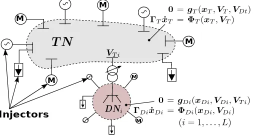
Figure 1. Decomposed Power System
II. SCHUR-COMPLEMENT-BASEDALGORITHM A. Model Decomposition
An important step in developing and applying a domain decomposition algorithm is the identification of the partition scheme to be used. In this paper, a topologically-based par-titioning has been chosen lying on the boundary between TN and DNs. The decomposition assumes that every DN is connected to a single TN bus through a transformer [4].
Let the power system sketched in Fig. 1 be decomposed into the TN and L DNs, along with the power system com-ponents connected to them. For reasons of simplicity, all the components connected to the TN or DNs that either produce or consume power in normal operating conditions (such as power plants, DGUs, induction motors, other loads, etc.) are calledinjectors.
The injectors’ model can be described by a system of non-linear DAEs [5]:
Γ ˙x=Φ(x,V)
where V is the vector of rectangular components of bus voltages (VDi if connected to thei-th DN orVT if connected
to the TN), x is the state vector containing differential and algebraic variables andΓ is a diagonal matrix with:
(Γ)ℓℓ=
(
0 if theℓ-th equation is algebraic
1 if theℓ-th equation is differential.
At the same time, under the standard phasor approximation, the algebraic equations of each network (TN or DN) take on the linear form:
0=DV −I,g(x,V)
whereD includes the real and imaginary parts of the bus ad-mittance matrix andIis the vector of rectangular components of the bus currents.
Hence, the DAE system describing the TN with its injectors is:
0=gT(xT,VT,VDt)
ΓTx˙T =ΦT(xT,VT) (1)
whereVDt is a sub-vector ofVD= [VD1. . . VDL]T,
includ-ing only the voltage components of the DN buses connected to the TN through the distribution transformers (see Fig. 1).
Similarly, for thei-th DN with its injectors (i= 1, . . . , L):
0=gDi(xDi,VDi,VT i)
ΓDix˙Di=ΦDi(xDi,VDi) (2)
where VT i is a sub-vector ofVT, including only the voltage
components of the TN bus where thei-th DN is connected to (see Fig. 1).
The proposed decomposition is reflected on the DAE sys-tems (1) and (2), through the common variablesVDtandVT i (i = 1, ..., L) involved in the equations of the distribution transformers connecting the DNs to the TN.
B. Discretization and Algebraization
For the purpose of numerical simulation, the injector DAE systems are discretized using a differentiation formula (such as Trapezoidal Rule, Backward Differentiation Formula, etc.) which yields the corresponding non-linear algebraized system:
0=f(x,V)
Next, these injector equations are linearized and solved together with the network equations using a Newton-type method to compute the state vectorsVT,xT,VDi andxDi.
Thus, at each Newton iteration, the linear system to be solved for the TN is:
JT1 JT2 JT3 JT4
| {z }
∆VT ∆xT
−PLi=1
CDi△VDi
0
=
JT −
gT(xT,VT,VDt)
fT(xT, VT)
(3)
where JT is the Jacobian matrix ofgT and fT towards the
TN states and CDi towards the voltage of the i-th DN. It is
worth noting that theCDi matrix is very sparse with the only
non-zero columns corresponding to voltage variables of DN buses directly connected to the TN through the transformers.
Similarly, for thei-th DN, it is:
JDi1 JDi2 JDi3 JDi4
| {z }
∆VDi ∆xDi
−
BDi△VT
0
=
JDi −
gDi(xDi,VDi,VT i)
fDi(xDi,VDi)
(4)
whereJDi is the Jacobian matrix ofgDiandfDitowards the
DNi states andBDi towards the TN bus voltage variables. It
can be seen that the BDi matrix is very sparse with the only
non-zero columns corresponding toVT i variables.
C. Reduced System Formulation
The solution of the systems (3)-(4) is performed in a de-composed manner using a Schur-complement-based method. For this, the systems (4) are each solved towards ∆VDi and
substituted in (3) to build a reduced system involving only the TN variables.
To solve for∆VDi, the system (4) can be rewritten as:
JDi1∆VDi + JDi2∆xDi = −gDi(xDi,VDi,VT i) +BDi△VT
" JT1−
PL
i=1CDiB˜Di JT2
JT3 JT4
# "
∆VT ∆xT
#
=− "
gT(xT,VT,VDt) +P L
i=1CDig˜Di(xDi,VDi,VT i)
fT(xT, VT)
#
(5)
and then solved for∆VDi as: ∆VDi = + SDi−1BDi△VT −S−Di1
gDi(xDi,VDi,VT i)
− JDi2JDi−14fDi(xDi,VDi)
= + ˜BDi△VT −g˜Di(xDi,VDi,VT i)
where:
SDi ,JDi1−JDi2JDi−14JDi3
˜
BDi ,S−Di1BDi ˜
gDi(xDi,VDi,VT i) ,S−Di1
gDi(xDi,VDi,VT i)
−JDi2J− 1
Di4fDi(xDi,VDi)
The resulting equations are then substituted in (3) to formulate the reduced system (5).
It should be noted that the Schur-complement terms CDiB˜Di each contribute a [2×2] matrix centered on the
diagonal ofJT1. Thus the original sparsity pattern of the TN Jacobian matrixJT is preserved. Also, each Right-Hand-Side
(RHS) factor CDig˜Di(xDi,VDi,VT i) affects only the
mis-match values of the TN bus where thei-th DN is connected, i.e. only two components when Cartesian coordinates are used. Finally, all the inverse matrix operations appearing in the above mathematical formulation are actually implemented as sparse linear system solutions, with appropriate solvers, to preserve computational efficiency.
D. Solution
The solution proceeds by solving the reduced system (5) to compute the corrections related to the TN. Then,∆VT and the
updatedVT variables are back substituted in Eqs. (4), which
are solved to compute the DN corrections. After updating the state vectors, if all the DAE systems (1)-(2) have been solved, the simulation proceeds to the next time instant, otherwise a new iteration is performed with the updated variables.
The solution algorithm performs a “dishonest” update of the Jacobian matrices. That is, the Jacobian matrices JT and
JDi, as well as the Schur-complement terms CDiB˜Di and
the intermediate matrices (e.g. SDi), are kept constant over
several solutions or even time-steps. They are selectively and independently updated only if the corresponding sub-network DAE does not converge after a number of iterations within the same discrete time computation.
The proposed algorithm is numerically equivalent to solv-ing the original DAE system (1)-(2) ussolv-ing a simultaneous Very DisHonest Newton (VDHN) method [6]. The Schur-complement-based algorithm, though, allows to selectively up-date the Jacobian matrices of DAE sub-systems when needed, and to exploit the decomposition to parallelize the procedure.
III. PARALLELCOMPUTINGASPECTS
Domain decomposition-based algorithms offer paralleliza-tion opportunities as independent computaparalleliza-tions can be
per-Parallel threads
Parallel threads
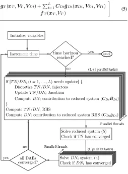
(L+1 parallel tasks)
[image:4.595.302.556.50.395.2](L parallel tasks)
Figure 2. Proposed Solution Algorithm
formed by different computing threads. The proposed algo-rithm, sketched in Fig. 2, employs parallel computing for the system formulation, Jacobian update and DN solution.
A. Parallel Algorithm
First, based on the proposed decomposition, no data depen-dencies exist in the system formulation of each sub-network (TN or DN). Thus, the independent calculations (injector discretization and linearization, Jacobian matrix update, mis-match and reduced system contribution evaluation) are each performed in parallel for the various sub-networks. This is shown in the upper shaded block in Fig. 2 where each parallel task deals with one sub-network. If the L+ 1 parallel tasks are more than the number of available computational threads, a sharing mechanism takes care of properly assigning the tasks to the threads.
be tackled with a parallel sparse linear solver, the overhead due to the new synchronization points would counteract the benefits. Hence, in this work, a sequential sparse linear solver has been used.
Finally, after the computed corrections∆VT are back
sub-stituted in Eqs. (4), the DN systems are decoupled, removing any data dependencies. The solution of DN sub-systems is obtained in parallel, using sparse linear solvers, and their convergence is checked. This is shown in the lower shaded block in Fig. 2 where each parallel task deals with one DN.
B. Implementation Specifics
Shared-memory, multi-core computers are becoming more and more popular among low-end and high-end users due to their availability, variety and performance at low prices. The OpenMP API was selected for this implementation as it is supported by most hardware and software vendors and it allows for portable, user-friendly programming.
OpenMP has the major advantage of being widely adopted, thus allowing the execution of a parallel application, with-out changes, on many different computers. It consists of a set of compiler directives, library routines, and environment variables that influence run-time behavior. A set of predefined directives are inserted in Fortran, C or C++ programs to describe how the work is to be shared among threads that will execute on different processors or cores and to order accesses to shared data [8].
One of the most important tasks is to make sure that parallel threads receive equal amounts of work. Imbalanced load sharing leads to delays, as some threads are still working while others have finished and remain idle. OpenMP includes three easy to employ mechanisms for achieving good load balance among the working threads [8].
First, with the static strategy, the scheduling is predefined and one or more parallel tasks are assigned to each thread rotationally prior to the parallel execution. This decreases the overhead needed for scheduling but can introduce load imbalance if the work inside each task is not the same. Second, with the dynamicstrategy, the scheduling is updated during the execution. This introduces a high overhead cost for managing the threads but provides the best possible load balancing. Finally, with the guided strategy, the scheduling is again dynamic but the number of tasks assigned to each thread are progressively reduced in size. This way, scheduling overheads are reduced at the beginning of the loop and good load balancing is achieved at the end.
In the proposed algorithm, high imbalance between parallel tasks can arise from the different sizes of the various sub-networks (TN or DNs). That is, if the sub-sub-networks in the system have different number of buses and injectors, hence different size of DAE systems, the threads computing them will have different work loads. In such situations, the dynamic strategy is preferred for better load balancing. Spatial locality can be addressed by defining a minimum number of successive tasks to be assigned to each thread (chunk). Temporal locality, on the other hand, cannot be easily addressed with this strategy
because the tasks treated by each thread, and thus the data accessed, are decided at run-time and can change from one parallel segment of the code to the next [8].
IV. RESULTS
In this section we present the results of the Schur-complement-based algorithm implemented in the academic simulation software RAMSES, developed at the University of Liège. The software is written in modern Fortran 2003 with the use of OpenMP directives for the parallelization as detailed in Section III. The simulations are performed on a 48-core AMD Opteron Interlagos1 desktop computer running Debian Linux 6. The environment variable OMP_NUM_THREADS
was used to vary the number of computational threads avail-able to the simulation software at each execution.
A. Performance Indices
Many different indices exist for assessing the performance of a parallel algorithm A. The two indices used in this study,
scalability andspeedup, are defined as [9]:
Scalability(N) = W all time(A) (1core)
W all time(A) (N cores) (6) Speedup(N) = W all time(V DHN) (1core)
W all time(A) (N cores) (7)
whereN is the number of available computational threads. The first index shows how the parallel implementation scales when the number of available processors increases. That is, the tested parallel algorithm is benchmarked against a sequential execution of thesamealgorithm.
The scalability index is directly related to Amdahl’s law [8] and using the latter, can be rewritten as:
Scalability(N) = S+P
S+P
N +OHC(N)
(8)
whereS is the sequentially computed portion,P the parallel portion andOHC the OverHead Cost of making the code run in parallel (creating and managing threads, communication, memory latency, etc.). The values ofSandPcan be estimated with the use of a profiler monitoring the sequential execution of the algorithm. Equations (6) and (8) can be used to assess the algorithm’s parallel efficiency, defined as the net incre-mental acceleration gained with each additional computational thread.
Usually, parallel algorithms are designed and optimized to be executed in parallel and exhibit low performance in sequen-tial execution. Thus, even though scalability is an important index, it is not enough to assess the absolute performance of a parallel algorithm. Hence, the speedup index (7) shows how much faster is the proposed parallel algorithm compared to a fast, optimized for sequential execution, algorithm. In this study, the sequential VDHN algorithm was used as a reference. In this algorithm, the combined DAE system (1)-(2)
g11 g20
g19
g16 g17
g18
g2 g9
g1 g3
g10 g5
g4
g12
g8
g13
g14 g7
g6
g15 4011
4012
1011
1012 1014 1013
1022 1021
2031
cs
4046 4043 4044
4032 4031
4022 4021 4071
4072
4041
1042
1045 1041
4063 4061
1043 1044
4047 4051
4045 4062
TN DN
NORTH
CENTRAL
EQUIV.
SOUTH
[image:6.595.302.557.52.193.2]4042 2032
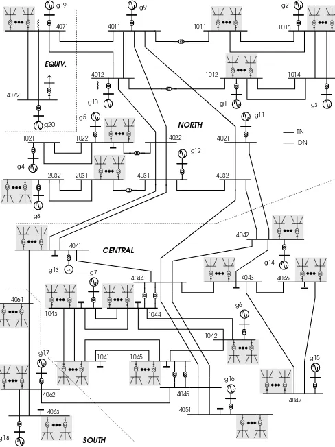
Figure 3. Expanded Nordic System
is solved as a whole using a Newton method with infrequent Jacobian update. The full DAE system is discretized and linearized, the combined Jacobian matrix is formulated and the linear system solved to compute all variable corrections simultaneously. The Jacobian matrix is updated only if the solution has not converged after three iterations. This is a well-known method used by many commercial and academic software and considered to be one of the fastest sequential algorithms [9].
It is noteworthy that both algorithms were implemented in the same software. Thus, they solve exactly the same model equations to the same accuracy, using the same algebraization method (namely the second-order backward differentiation for-mula), way of handling the discrete events [10], mathematical libraries (i.e. sparse linear solver), etc. Keeping the aforemen-tioned parameters the same for both algorithms permits for the better evaluation of the proposed algorithm’s performance.
B. Test System Model
This section reports on results obtained with a large-scale combined transmission and distribution network model based on the Nordic system, documented in [11]. The original TN model is extended with 146 realistic DNs replacing its aggregated distribution loads as shown in Fig. 3. The model and data of each DN were taken from [12] and scaled to match
0.96 0.97 0.98 0.99 1 1.01 1.02
0 20 40 60 80 100 120 140 160 180
t (s) (pu)
VDHN Parallel Algorithm
Figure 4. Case 1: Voltage on TN bus 1041
the original TN loads. Multiple DNs were used to match the original load powers, taking into account the nominal power of the TN-DN transformers.
Each one of the 146 DNs includes 100 buses, 108 branches, one distribution voltage regulator equipped with Load Tap Changing (LTC) device, three type-1, three type-2 and two type-3 Wind Turbines (WTs) [13], 12 impedance loads and 133 dynamically modeled loads, such as small induction machines and self-restoring exponential loads. The transformer connecting each DN to the TN is also equipped with an LTC controlling the distribution side voltage.
To further avoid identical DNs and artificial synchroniza-tion, the delays on transformer tap changes were randomized around their original values and the WTs were randomly initialized to produce 80-100% of their nominal power.
In total, the combined transmission and distribution sys-tem includes 14653 buses, 15994 branches, 20 synchronous machines, 293 LTC equipped transformers, 1168 WTs, 1752 impedance loads and 19419 dynamically modeled loads. The resulting DAE system has 143462 differential-algebraic states.
C. Case 1
The disturbance considered in this scenario is the loss of approximately 115 MW of wind generation due to the disconnection of 30 type-1, 30 type-2 and 20 type-3 WTs located inside ten DNs, all connected to TN bus 1041 in the CENTRAL area (see Fig. 3). The WTs, grouped per DN, are successively disconnected over a period of 10 s and the system is simulated for 180 s with a time-step size of one cycle at the nominal frequency (50 Hz). This event might result from high winds in the area, causing WTs to trip to avoid damage. Such disturbances, with events happening inside the DNs, are very difficult to simulate when detailed DN models are not used.
[image:6.595.43.287.54.380.2]-80 -75 -70 -65 -60 -55
0 20 40 60 80 100 120 140 160 180 t (s)
(MW)
DNA DND DNF
Figure 5. Case 1: Active power transfer over TN-DN transformers
(negative sign signifies the DN is importing active power from the TN)
voltages, thus further depressing TN voltages. The simulated evolution is shown with both VDHN and the proposed parallel algorithm. As expected, the output trajectories are indistin-guishable as the two algorithms solve the same DAEs with the same accuracy.
Figure 5 shows the active power transfer over the TN-DN transformers of three of the TN-DNs. In particular, TN-DNA
is the first, DND is the fourth and DNF the sixth whose
WTs disconnect. When the WTs of a DN disconnect, the imported power is immediately increased to compensate for the lost local generation. The already mentioned TN voltage drop impacts the neighboring DNs and, due to the voltage sensitivity of loads, the imported power decreases. Hence, immediately after the disturbance, only a fraction of the lost WT power is imported from the TN. In the long-term, as the LTC actions restore the DN voltages, the load consumption is also restored and the whole lost active power deficit is compensated by importing from the TN.
This interaction mechanism shows the necessity for detailed DN representation in dynamic simulations. The sequence of discrete events, like WT disconnections, LTC actions, etc., the behavior of DN components and controls, and the interactions of DNs with the TN or between them, dictate the resulting system evolution.
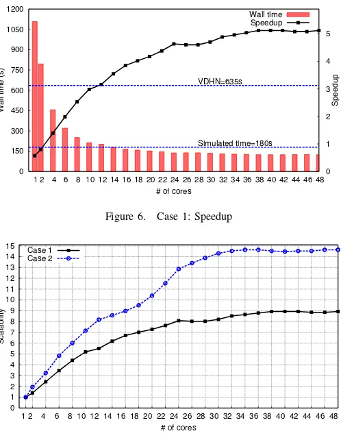
Figure 6 shows that algorithmA offers a speedup of up to 5.2 times when compared to the VDHN algorithm. Initially, the parallel algorithm executed on a single core performs around 40% slower than the, optimized for sequential execution, VDHN. This delay is due to the extra computational costs of the domain decomposition-based scheme (e.g. partition-related book-keeping, intermediate Schur-complement calculations, etc.). As regards the scalability of the algorithm, Fig. 7 shows that it executes up to nine times faster in parallel compared to its own sequential execution.
From Figs. 6 and 7, it can be seen that the parallel algorithm is more efficient in the range of up to 24 cores, while after that the benefit becomes marginal. This can be explained from Eq. (8). When increasing the number of parallel threads by one, the execution time gained can be computed as NP −
P
N+1, assuming that the sequential and
0 150 300 450 600 750 900 1050 1200
1 2 4 6 8 10 12 14 16 18 20 22 24 26 28 30 32 34 36 38 40 42 44 46 48 0 1 2 3 4 5
Wall time (s) Speedup
# of cores
Simulated time=180s VDHN=635s
[image:7.595.306.555.51.372.2]Wall time Speedup
Figure 6. Case 1: Speedup
0 1 2 3 4 5 6 7 8 9 10 11 12 13 14 15
1 2 4 6 8 10 12 14 16 18 20 22 24 26 28 30 32 34 36 38 40 42 44 46 48
Scalability
# of cores Case 1
Case 2
Figure 7. Case 1 and 2: Scalability
parallel portions remain unchanged. Thus, whenN increases, it is easy to see that the incremental gain decreases. At the same time, the incremental OHC of creating and managing a new thread(OHC(N + 1)−OHC(N)), calculated for the specific computer platform, is almost constant. Hence, as the number of computational threads increases, the net incremental gain (difference between incremental gain andOHC) declines and can reach zero or even negative values.
D. Case 2
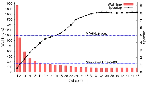
The disturbance considered in this scenario is a five cycle (0.1 s) short circuit near the TN bus 4032 cleared by the opening line 4032-4042. The system is then simulated over 240 s with one cycle time-step size. After the electromechan-ical oscillations have died out, the system evolves in the long-term under the effect of LTCs acting to restore distribution voltages and overexcitation limiters on the generators. This is a severe disturbance that affects all the TN and DNs.
Figure 8 shows the active power output of a type-3 WT located in one of the DNs of the CENTRAL area. It is shown with both VDHN and the proposed parallel algorithm. As expected, the two are indistinguishable.
[image:7.595.40.294.53.194.2]1.42 1.43 1.44 1.45 1.46 1.47 1.48
0 40 80 120 160 200 240
t (s) (MW)
[image:8.595.302.554.52.198.2]VDHN Parallel Algorithm
Figure 8. Case 2: DN type-3 WT active power output
It can be seen that both scalability and speedup are higher in Case 2 compared to Case 1. Moreover, the algorithm exhibits efficient scaling up to 32 cores, compared to the 24 cores of the previous case. These differences can be explained by the larger amount of computational work available in the parallel portion of this simulation. Indeed, due to the severe nature of this scenario, the system exhibits higher dynamic activity. Thus, more frequent Jacobian matrix updates and more DN system solutions are required, leading to an increased overall computation time (S+P). At the same time, as most of the aforementioned computations are in the parallel portion, the ratio SP+P also increases. Hence, with a biggerP value, the
higher scalability and speedup achieved can be explained from Eq. (8), considering that the incrementalOHC, that depends on the computer platform, is the same as before.
In general, the proposed algorithm is more efficient and achieves higher speedup when simulations with high dynamic activity are considered.
V. CONCLUSION
In the future, distributed protection and control schemes, DGUs providing ancillary services and active demand re-sponse will make the contribution of DNs to the system dynamics more significant and their detailed simulation more vital. Thus, the need for simulating larger power system models, including DNs, will increase the computational burden of dynamic simulations.
In this paper a parallel Schur-complement-based algorithm for dynamic simulation of combined transmission and dis-tribution systems has been presented. The algorithm yields acceleration of the simulation procedure in two ways. On the one hand, the procedure is accelerated numerically, by performing selective and infrequent Jacobian updates of the decomposed sub-systems. On the other hand, it is accelerated computationally, by exploiting the parallelization opportunities inherent to domain decomposition algorithms.
The proposed algorithm is accurate, as the original system of equations is solved with the same accuracy. It has the ability to simulate a wide variety of disturbances. It exhibits high numerical convergence rate, provided by Newton-type algorithms.
0 150 300 450 600 750 900 1050 1200 1350 1500 1650 1800 1950
1 2 4 6 8 10 12 14 16 18 20 22 24 26 28 30 32 34 36 38 40 42 44 46 48 0 1 2 3 4 5 6 7 8 9
Wall time (s) Speedup
# of cores
Simulated time=240s VDHN=1053s
[image:8.595.43.294.56.193.2]Wall time Speedup
Figure 9. Case 2: Speedup
Along with the proposed algorithm, an implementation based on the shared-memory parallel programming model has been presented. The implementation is portable, as it can be executed on any platform supporting the OpenMP API. It can handle general power systems, as no hand-crafted, system specific, optimizations were applied. Finally, it exhibits good parallel performance on inexpensive, shared-memory, multi-core computers.
REFERENCES
[1] D. Koester, S. Ranka, and G. Fox, “Power systems transient stability-A grand computing challenge,”Northeast Parallel Architectures Center, Syracuse, NY, Tech. Rep. SCCS, vol. 549, 1992.
[2] R. Green, L. Wang, and M. Alam, “High performance computing for electric power systems: Applications and trends,” inProc. of IEEE PES General Meeting, 2011.
[3] U. D. Annakkage, N. K. C. Nair, Y. Liang, A. M. Gole, V. Dinavahi, B. Gustavsen, T. Noda, H. Ghasemi, A. Monti, M. Matar, R. Iravani, and J. A. Martinez, “Dynamic System Equivalents: A Survey of Available Techniques,”IEEE Transactions on Power Delivery, vol. 27, pp. 411– 420, Jan. 2012.
[4] T. Short, Electric Power Distribution Handbook. Electric power engi-neering series, Taylor & Francis, 2003.
[5] P. Kundur,Power system stability and control. McGraw-hill New York, 1994.
[6] B. Stott, “Power system dynamic response calculations,”Proceedings of the IEEE, vol. 67, no. 2, pp. 219–241, 1979.
[7] Y. Saad, Iterative methods for sparse linear systems. Society for Industrial and Applied Mathematics, 2nd ed., 2003.
[8] B. Chapman, G. Jost, and R. Van Der Pas,Using OpenMP: Portable Shared Memory Parallel Programming. MIT Press, 2007.
[9] J. Chai and A. Bose, “Bottlenecks in parallel algorithms for power system stability analysis,”IEEE Transactions on Power Systems, vol. 8, no. 1, pp. 9–15, 1993.
[10] D. Fabozzi, A. Chieh, P. Panciatici, and T. Van Cutsem, “On simplified handling of state events in time-domain simulation,” inProc. of the 17th Power Systems Computation Conference, 2011.
[11] T. Van Cutsem, “Description, modeling and simulation results of a test system for voltage stability analysis,” Internal Report, University of Liège, Sept. 2013. http://hdl.handle.net/2268/141234.
[12] A. Ishchenko, Dynamics and stability of distribution networks with dispersed generation. PhD thesis, Dept. Electrical. Eng., Univ. TU/ E, the Netherlands, 2008.