This is a repository copy of Dynamic portfolio optimization with transaction costs and state-dependent drift.
White Rose Research Online URL for this paper: http://eprints.whiterose.ac.uk/83104/
Version: Accepted Version
Article:
Palczewski, J, Poulsen, R, Schenk-Hoppé, KR et al. (1 more author) (2015) Dynamic portfolio optimization with transaction costs and state-dependent drift. European Journal of Operational Research, 243 (3). pp. 921-931. ISSN 0377-2217
https://doi.org/10.1016/j.ejor.2014.12.040
© 2015. This manuscript version is made available under the CC-BY-NC-ND 4.0 license http://creativecommons.org/licenses/by-nc-nd/4.0/
Reuse
Unless indicated otherwise, fulltext items are protected by copyright with all rights reserved. The copyright exception in section 29 of the Copyright, Designs and Patents Act 1988 allows the making of a single copy solely for the purpose of non-commercial research or private study within the limits of fair dealing. The publisher or other rights-holder may allow further reproduction and re-use of this version - refer to the White Rose Research Online record for this item. Where records identify the publisher as the copyright holder, users can verify any specific terms of use on the publisher’s website.
Takedown
If you consider content in White Rose Research Online to be in breach of UK law, please notify us by
Dynamic portfolio optimization with transaction costs
and state-dependent drift
I,IIJan Palczewski
School of Mathematics, University of Leeds, UK.
Rolf Poulsen
Department of Mathematical Sciences, University of Copenhagen, Denmark.
Klaus Reiner Schenk-Hopp´e
Leeds University Business School and School of Mathematics, University of Leeds, UK. Department of Finance, NHH–Norwegian School of Economics, Norway.
Huamao Wang∗
School of Mathematics, Statistics and Actuarial Science, University of Kent, UK.
Abstract
The problem of dynamic portfolio choice with transaction costs is often ad-dressed by constructing a Markov Chain approximation of the continuous time price processes. Using this approximation, we present an efficient
nu-IThe authors are grateful to the two anonymous reviewers and the editor, Professor
Immanuel Bomze, for their helpful comments and advice.
IIThe paper benefitted from the first and third authors’ visits to the Hausdorff Research
Institute for Mathematics at the University of Bonn in the framework of the Trimester Program Stochastic Dynamics in Economics and Finance. The second author gratefully acknowledges support from the Danish Strategic Research Council under contract number 10-092299, the research center ‘HIPERFIT’. The fourth author acknowledges support from Kent Faculty of Sciences Research Fund.
∗Corresponding author. Tel: +44 1227 823593; Fax: +44 1227 827932.
Email addresses: [email protected](Jan Palczewski),[email protected]
(Rolf Poulsen), [email protected](Klaus Reiner Schenk-Hopp´e),
merical method to determine optimal portfolio strategies under time- and state-dependent drift and proportional transaction costs. This scenario aris-es when invaris-estors have behavioral biasaris-es or the actual drift is unknown and needs to be estimated. Our numerical method solves dynamic optimal port-folio problems with an exponential utility function for time-horizons of up to 40 years. It is applied to measure the value of information and the loss from transaction costs using the indifference principle.
Keywords: Dynamic programming, numerical methods, state-dependent
drift, transaction costs, Markov Chain approximation
JEL: C61, C63, G11
1. Introduction
Numerical methods for dynamic portfolio optimization under proportion-al transaction costs typicproportion-ally assume that the drift of the risky asset is con-stant. However, a state-dependent drift enters the optimization problem in many scenarios. For instance, if the drift is unobservable, it can be estimated with the Kalman-Bucy filter. This leads to an optimization problem where the drift depends on the currently observed stock price (e.g. Bj¨ork et al. 2010). The drift is also state-dependent when contrarian investors optimize portfolios under the assumption that prices are mean-reverting; for instance when an investor is a victim of the Gambler’s fallacy, see, e.g.,Shefrin(2008). Similarly, investors who aim at following market trends will include a state-dependent drift in optimization.
nu-merically demanding problem. Our paper proposes an efficient numerical method to solve finite-horizon portfolio optimization problems with trans-action costs and state-dependent drift. The method has time-complexity of O(N2.5), where N is the number of time steps in the discrete approximation
of the investment interval. In contrast, a discrete-time dynamic program-ming algorithm (see (8) in Section 3) that directly solves the problem has time-complexity O(N5). Our method allows us, for instance, to study
40-year investment horizons with time steps of 4-day length on a basic laptop computer.
There are several numerical methods for solving the optimization problem with a constant drift under transaction costs. Davis et al. (1993) proposes a backward recursive method which has seen a number of improvements in the past 20 years. For instance, Monoyios (2004) provides an approxima-tion to the optimal decision in the final period which allows searching over a smaller range of stock holdings. Zakamouline (2005) proposes bounds on stock holdings. Another method is to solve the Hamilton-Jacobi-Bellman (HJB) equations of optimization problems by finite differences (e.g. Herzog
et al. 2013) or to use a genetic programming algorithm to derive
approx-imations of trading strategies (Lensberg and Schenk-Hopp´e 2013). These algorithms work well for short time-horizons, typically less than one year, and when the number of periods is small. By proposing a method that works for non-constant drift and long time-horizons, our paper fills this gap in the literature.
tree, and that the state-dependent strategy results in a larger range of stock holdings. This increases the likelihood of over- and underflow arising for the exponential utility function as pointed out by Clewlow and Hodges (1997). For a constant drift, in contrast, the optimal strategy is independent of stock prices at time t. One only needs to search for the optimal strategy at a node at time t, see Monoyios (2004, p. 902).
To overcome the challenges, we develop a fast numerical method to ap-proximate the optimal solution well. The approach combines four aspects: (a) reducing dimensionality, (b) scaling the objective function, (c) carrying out local searches for optimal trading decisions, and (d) non-equidistant dis-cretization of the state space.
We apply the numerical method to a study of the true costs of market frictions using the indifference principle. The analysis reaps the full benefit of the approach because measuring these costs requires taking averages over many realizations of the drift. For each realization, one has to calculate trading strategies and carry out Monte Carlo simulations. In general, a state-dependent drift is observed to make the strategy more variable than a constant drift. This, in turn, entails more aggressive trading.
The indifference principle yields the following results.
First, the value of information is measured by comparing realized utilities of different types of investors. We find that information is most valuable to the least risk-averse investor. It also turns out that cautious trend-followers do almost as well as investors who estimate the drift from observations.
trans-action costs. The loss is observed to be about twice as large as the direct expense incurred. Transaction costs are most detrimental to naive investors (who do not revise their initial estimates of the drift) when investing over a medium or long time horizon. It implies that in the long run naive in-vestors are the most active traders and usually hold wrong beliefs. At short time-horizons, transaction costs strongly affect the learning investor as his estimate of the drift varies drastically in the short run.
Third, we examine the impact of the investment time horizon. The main finding is that, although uncertainty about the true drift cannot be removed completely, learning about the drift reduces the loss in utility due to the uncertain drift by 33% in one year and by 80% in ten years compared to a naive investor. Learning also reduces the loss in utility caused by transaction costs by 50% over a 10-year time-horizon.
Section 2 presents the model. The numerical method is explained in Section 3 and applied in Section 4 to quantify the economic costs under various assumptions on the state-dependent drift. Section 5 concludes.
2. Model
We consider an investor who maximizes utility from wealth by trading in a risk-free bond with a constant interest rate r, and a risky stock. The randomness of the stock price is modelled on a probability space (Ω,F,P)
which supports a one-dimensional Brownian motion (W(t)) and an indepen-dent random variable m whose role will be explained later. The investor assumes that the dynamics of the stock price S(t) is given by
with a constant volatility σ > 0. The function µ(t, S) is a time- and state-dependent drift of the stock price.
We consider a situation in which the true dynamics of the stock price is unknown: The actual drift is a random variable m which is determined at the initial time and fixed over the horizon (recall that it is independent of the Brownian motion (W(t))). Hence the true price dynamics is
dS(t) = mS(t)dt+σS(t)dW(t). (2)
The drift m is not observed by investors with an exception of an informed investor (a benchmark) who additionally knows the drift m. If the structure of the price dynamics is known, one can use observed stock prices to estimate m. Assume throughout the paper thatm is normally distributed with mean µ0 and variance γ0 >0:
m ∼ N(µ0, γ0).
Then the Kalman-Bucy filter gives that the best estimate of m given an observation of the stock price trajectory up to time t is
µL(t, S(t)) = γ0σ
2
σ2+γ 0t
( µ0 γ0
+ t 2+
1
σ2 log(S(t)/S0)
)
. (3)
This estimate takes the form µ(t, S(t)), and hence entails a dynamics as defined in (1).
second type of investor suffers from a behavioral bias and estimates the drift as:
µa(t, S(t)) = µ0+a arctan
(
(µ0 −σ2/2)t−log(S(t)/S0)
)
. (4)
The second item of (4) characterizes the investor’s adjustment to his initial estimate µ0. The arctangent function is a symmetric about the origin
and increasing function taking values within (−π/2, π/2) on the domain (−∞, +∞), see, e.g. Luderer et al. (2010, p. 55). The adjustment vanishes when the logarithmic returnR(t) := log(S(t)/S0) equals (µ0−σ2/2)t which
was the expected value E[R(t)] if the drift of the stock price was a known
constant µ0. In this case, it is known that, see, e.g. Øksendal (2003, p. 64)
R(t) := log(S(t)/S0) = (µ0−σ2/2)t+σ W(t).
We refer to the parameter ‘a’ as the investor’ssentiment. It measures the investor’s confidence in his initial estimateµ0. If the parameter a is positive
then the investor believes that the price will revert to the predicted mean: A higher than predicted return is forecast to lead to a drift smaller than µ0.
The investor’s decision is contrarian. It can be interpreted as the result of overconfidence about the ability to predict the stock price dynamics. If the parameter a is negative, the investor will revise the initial estimate upwards if the returns are higher than predicted (resp. downwards if returns are lower thanµ0). The investor is a trend follower; he places more trust in the market’s
view about stock price dynamics than in his own view.
Definition 2.1. Informed investors observe the realization of the random
Learninginvestors use (3)to estimate the realization of the random drift
m.
Naive investors assume that the drift is constant m=µ0.
Biased investors use (4) as their estimate of the drift.
Trading in the stock incurs proportional transaction costs with the rate λ ∈ [0,1). Purchasing y shares costs y(1 + λ)S(t) at time t while selling y shares brings in y(1− λ)S(t). It is customary (e.g. Davis et al. 1993) to describe an investor’s trading strategy with two non-decreasing right-continuous processes L(t) and M(t) representing, respectively, the cumula-tive number of shares bought and sold over [0, t]. The dynamics of portfolio positions (x(t), y(t)), where x(t) is the value of bonds held and y(t) is the number of shares, is
dx(t) = rx(t)dt−(1 +λ)S(t)dL(t) + (1−λ)S(t)dM(t), dy(t) = dL(t)−dM(t).
Given an initial position (x0, y0), the investor maximizes the expected
utility of the terminal wealth by following a trading strategy (L(t), M(t)):
max
(L,M)
E{U(x(T) +y(T)S(T))}.
We impose two standard assumptions: there are no liquidation costs of the portfolio at the terminal time T and the investor has a utility function with a constant absolute risk aversion (CARA) coefficient α:
U(w) =−exp(−αw). (5)
that it is optimal to estimate the true drift using (3) and to solve the optimization problem under the stock price dynamics given by (1) with µ(t, S(t)) = µL(t, S(t)).1 Biased investors’ optimization problem mimics be-havioral decision making.
Stochastic differential equations with drift of the form (3) or (4) do not satisfy the standard conditions for existence and uniqueness of solution. We therefore provide a result that establishes existence of a unique solution.
Lemma 2.2. Assume that µ: [0, T]×(0,∞)→R is a continuous function
that satisfies a logarithmic growth condition
|µ(u, S)| ≤M(1 +|log(S)|), S >0, u∈[0, T],
and a logarithmic Lipschitz condition
|µ(u, S1)−µ(u, S2)| ≤M|log(S1)−log(S2)|, S1, S2 >0, u∈[0, T]
for some constant M > 0. Then there is a unique strong solution to the
stochastic differential equation (1) for every initial condition S > 0.
Proof. Øksendal (2003, Theorem 5.2.1) implies that under the assumptions
of the lemma there is a unique strong solution to the stochastic differential equation
dZ(u) = (µ(u, eZ(u))− σ 2
2 )
du+σdW(u), Z(t) = 0. (6)
1
By Itˆo’s formula the process S(u) = S(t)eZ(u)−Z(t),u≥t, satisfies (1), i.e., it
is a strong solution to this equation. To prove uniqueness, assume that there is another strong solution to (1), denoted by ¯S(u), u ≥t, with ¯S(t) = S(t) and ¯S(u) ̸=S(u) for u > t. Define ¯Z(u) = log( ¯S(u)/S¯(t)). Again, by Itˆo’s formula ¯Z(u) satisfies (6) and is different from Z(u). This contradicts the
uniqueness of the solution to (6).
Let us verify that the drifts of the forms (3) and (4) satisfy assumptions of the above lemma. We have
|µL(u, S1)−µL(u, S2)| ≤ γ0
σ2|log(S1)−log(S2)|,
and
|µL(u, S)| ≤sup
t≥0
|µL(t, S)|
≤sup
t≥0
{ γ0σ2 σ2+γ
0t ( µ0 γ0 + t 2 + 1
σ2|log(S0)|
)} + sup
t≥0
{ γ0σ2 σ2+γ
0t
1
σ2 log(S)
}
≤ γ0
σ2|log(S0)|+ σ2
2 +µ0+ γ0
σ2|log(S)|.
For a biased investor, we obtain
|µa(u, S)| ≤µ0+|a| π 2, and
|µa(u, S1)−µa(u, S2)| ≤ |a| sup
x∈(−∞,∞)
|arctan′(x)||log(S
1)−log(S2)|
≤ |a||log(S1)−log(S2)|.
investor whose portfolio at time t consisting ofx value of bond and y shares of the stock priced at S(t) = s:
V(t, s, x, y) = sup
(L(u),M(u))u≥t
E{U(x(T)+y(T)S(T))|(S(t), x(t), y(t)) = (s, x, y)}.
In the simplest case when the drift functionµ(t, s)≡µ¯(a constant), the value function is characterized as a unique viscosity solution of an HJB equation
(Davis et al. 1993):2
max{Vt+rxVx+ ¯µsVs+
σ2
2 s
2V
ss;
Vy−(1 +λ)sVx; −Vy+ (1−λ)sVx
} = 0
(7)
with the terminal condition V(T, s, x, y) = U(x+ys) (subscripts in (7) de-note partial derivatives). Solving this equation is usually carried out using numerical approximation. For general drift functions,anHJB representation is not known. We therefore take a different route to study optimal invest-ment when the drift function is time- and state-dependent. In this paper, approximations are designed for the stochastic control problem itself.
3. Numerical Approach
We apply Bellman’s dynamic programming principle to solve the control problem with state-dependent drift. The stock price model is discretized in time and space, and the programming works recursively backwards in time. Let time be discretized in steps of length ∆t with ∆t = T /N where N is the number of time steps. At each time-point the investor has to choose
2
whether to trade and, if yes, how many units of stock to trade. The bond holdings are determined by the self-financing condition. The expected utility derived from each possible trading choice is determined by the value function. To select the trading decision that maximizes expected utility, the investor solves the maximization problem:
V(t, s, x, y) = max{E(V(t+ ∆t, S(t+ ∆t), er∆tx, y)|S(t) =s)
| {z }
benefit from not trading, ∆y= 0 ,
max
∆y>0
E(V(t+ ∆t, S(t+ ∆t), er∆t(x−∆y×s(1 +λ)), y+ ∆y)|S(t) =s)
| {z }
benefit from buying ∆y >0 shares
, (8)
max
∆y>0
E(V(t+ ∆t, S(t+ ∆t), er∆t(x+ ∆y×s(1−λ)), y−∆y)|S(t) =s)
| {z }
benefit from selling ∆y >0 shares
}
where the maximization is over the type of trade and the corresponding volume to be traded.
One might conjecture that the spatial discretization of the stock price process is complicated when its drift is state-dependent. However, one can use a standard binomial tree approximation of Cox et al. (1979) and define adjusted probabilities for the up- and down-movement of the discretized stock price. This Markov Chain approximation is provided in, e.g., Kushner and
Dupuis (1992) and Zakamouline(2005). The benefit of this representation is
that the stock-price model retains the property of being a recombining tree. Specifically, we use the following binomial model. Define the coefficients u= 1/d=eσ√∆t, and set the process
S(t+∆t) =
uS(t) with probability p(t, S(t)) = [eµ(t,S(t))∆t−d]/[u−d], dS(t) with probability 1−p(t, S(t)).
is given by the set Mx×My with Mx ={xj :xj =x+jδx≤x, j¯ ∈N} and
My = {yk : yk = y+kδy ≤ y, k¯ ∈ N} with given x, ¯x, y, and ¯y, where δx
(resp.δy) is the grid spacing in the dimension of money (resp. stock holdings). A direct algorithm for determining the value function and the optimal trading strategy proceeds as follows.
Define the value function at the terminal time as the realized utility. Set
V(T, s, xj, yk) :=U(xj+yks) for all valuess of the discretized stock prices
in period T and all portfolio holdings (xj, yk)∈Mx×My.
For t =T −∆t, ...,0
For all values of the discretized stock price s=S(t) at time t
For all values (xj, yk)∈Mx×My
Given the functionsV(t+ ∆t, ...), find the highest value in (8)
obtained over all values ∆y such that yk+ ∆y∈ My3. Denote
the maximum value V(t, s, xj, yk).
End For
End For
End For
The computational complexity of the direct method is of the orderO(N2× Mx ×My ×My) or O(N5).4 The factor N2 arises because the algorithm
loops through all points on the stock price lattice, the factor Mx×My is due
to the loop through the grid of portfolio holdings, and the final factor My
3
V(t+∆t, ...) is approximated via a linear interpolation because exp(r∆t)[xj∓∆ys(1±
λ)] is typically not an element ofMx.
4
We letMx andMy linearly depend on time stepsN to ensure that the grid sizesδx
comes from the ∆y-search. This is slow; doubling the number of steps in all dimensions increases computation time by a factor of 32.
The range ofMx×My is usually large in order to include optimal solutions
for all possible states (t, S(t)) on the lattice. The above direct numerical method uses a standard equidistant grid and searches for optimal solutions in the whole set.
As a benchmark, suppose the direct algorithm is implemented in a high-level language such as Matlab on a typical laptop computer. Pricing an option on a binomial lattice with T = 1 year and time steps of 1 day takes 5 - 10 milliseconds, while on the lattice doing optimization over a grid of Mx×My = 100×100, i.e. O(Mx×My2) =O(106), takes about 2 hours. This
is not a computationally feasible approach since reasonable outputs require high-resolution grids and thousands of simulations of a random drift.
Five measures are employed to reduce running time of simulations:
Reducing dimension. When measuring utility by the negative
expo-nential function (5), the value function V can be written in the form
V(t, s, x, y) =H(t, s, y) exp (−αxexp(r(T −t))), (9)
where H(t, s, y) is defined by H(t, s, y) := V(t, s,0, y), see, e.g., Davis et al.
(1993) or Monoyios (2004). This representation allows reducing the
nu-merical over- or underflow errors in the computer program, which are dealt with by our following function H(t, s, y) scale, along with local search and non-equidistant discretization that speeds up the program.
Scaling the functionH(t, s, y). To mitigate over- and underflow issues, the value function H(t, s, y) is scaled:
G(t, s, y) := V(t, s,−ys, y) =H(t, s, y) exp (αysexp(r(T −t))).
Function G satisfies a discrete time dynamic programming equation similar to (8) with the terminal condition G(T, s, y) = −1.
Local∆y-search. The solution toH(t, s, y) is known to have a particular structure. The space of stock holdings is split into three regions: buy, no-trade and sell. If the stock position is either in the buy or sell region, a trade is initiated that leads to a stock position on the closest boundary of the no-trade region. If the stock position is inside or on the boundary of the no-trade region, the investor does not change his stock position.
In the case of a constant drift (Monoyios 2004, p. 902) the upper boundary (above which one sells) and the lower boundary (below which one buys) of the no-trade region at a given time t can be both defined by market values of stock positions. It is therefore sufficient to determine the optimal trade in all time-t nodes with a node (t, S) to find the two boundaries.
deter-mine the boundaries of the no-trade region through searching over a local range of y. One can also use a binary search algorithm as in Zakamouline
(2005) to improve computational speed further. The local range denoted by [φb(t, S), φs(t, S)] is determined by an appropriate extension of the
bound-aries at the successive nodes5.
Non-equidistant y-discretization. The structure of optimal trading
strategies suggests that it is not efficient to have an equidistant discretization of the y-space. The set of discretization points should be denser close to the boundaries of the no-trade region. We therefore use a symmetric, non-equidistant discretization.
The set is centered at Merton’s closed-form solution for the case of a constant drift and no transaction costs, which is denoted by φM(t, S). The
value of driftµis given by investors (possibly an actual value or an estimate). The non-equidistant grid has larger step-sizes away from the centerφM(t, S).
For a given (t, S)-node and the local range [φb(t, S), φs(t, S)], we first define
the radius
Φ(t, S) := max{φM(t, S)−φb(t, S), φs(t, S)−φM(t, S)}, (10)
5
Denoting the buy (resp. sell) boundary byyb (resp.ys) we identify the endpoints by
φb(t, S) = min{yb(t+ ∆t, d S(t)), yb(t+ ∆t, u S(t))} −C1,
φs(t, S) = max{ys(t+ ∆t, d S(t)), ys(t+ ∆t, u S(t))}+C2,
where C1 and C2 are two positive constants selected to ensure the local range is large
enough. We check whether the no-trade boundaries obtained numerically hit the endpoints of the local range. If they do, larger values ofC1andC2are chosen and the corresponding
where
φM(t, S) =
µ−r er(T−t)α σ2S
is the Merton solution. Then we define the set of discretization points as:
y(t, S, k) =φM(t, S) +
Φ(t, S) (
My
2
)ϖ
(
k− My
2 ) k− My 2
ϖ−1
. (11)
The coefficient ϖ > 1 controls the level of dispersion.6 Numerical experi-ments (see Wang (2010, Sect. 3.6.4) for details) show that an appropriate choice of the coefficient ϖ is 1.6.
Low-level language. Implementation in a low-level language, e.g.,
C++, reduces computation time by a factor of approximately 10.
Numerical illustration. We use the following values of parameters as
a base case for our numerical results: the actual drift drawn from the normal distribution with meanµ0 = 0.15 and varianceγ0 = 0.04, volatilityσ= 0.25,
proportional transaction cost rate λ= 0.01, initial stock price S0 = 15, risk
aversion α = 0.1, interest rate r = 0.03, time-horizon T = 1 year, and discretization parameters ∆t= 0.01, My = 3,500 and ϖ = 1.6.
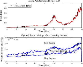
Figure 1 demonstrates the joint effect of transaction costs and state-dependent drift. It shows one realization of the optimal trading strategy over a 40-year time-horizon. The effect is substantial as evidenced by the high variability of the boundaries of the no-trade region. The volatility of
6
0 5 10 15 20 25 30 35 40 0
200 400 600 800 1000
Time (Year)
Stock Price
Stock Path Generated by µ = 0.15
Transaction Time
0 5 10 15 20 25 30 35 40
−10 0 10 20 30
Time (Year)
Wealth Invested in Stocks
Optimal Stock Holdings of the Learning Investor
Ntrans = 94
Sell Region
No−Trade Region
[image:19.612.147.468.131.391.2]Buy Region
Figure 1: Dynamics of the no-trade region with state-dependent driftµL(t, S(t))
within T = 40 years horizon. The squares indicate transaction times. Ntrans is
the total number of transactions.
these boundaries reflects changes in the learning investor’s estimate of the drift. For instance, both boundaries move downwards around year 25-30 in response to a pronounced fall in the stock price. They move upwards again around year 32 when the stock price recovers. With a known, constant drift, these boundaries (when measured in terms of the amount of wealth invested in stocks) are hyperbola-like curves that are independent of the stock price.
Comparison withMonoyios(2004)’s results. Verification of our method is
carried out by comparing numerical results with those reported inMonoyios
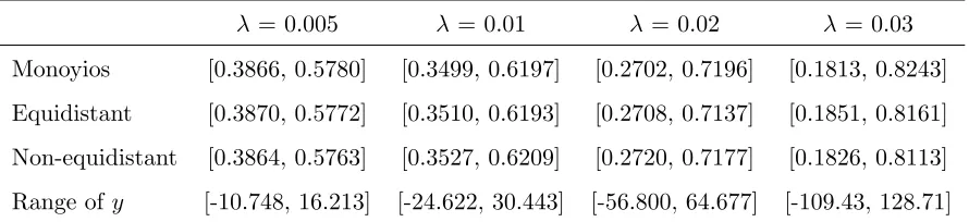
which is considered in the latter paper. Table 1 reports the two boundaries of the no-trade region at the initial time for different transaction costs. We calculate results with our method under both equidistant and non-equidistant discretization. In all three scenarios and for different transaction costs the calculated boundaries coincide up to 3-4 significant digits.
The non-equidistant discretization requires fewer points on the y-grid than the equidistant discretization, which substantially shortens the run-time of the program. Our approach works efficiently because we take state-dependent non-equidistant discretization on a small local range of y-values. In fact, the discretization equation (11) produces a great number of dense points with the precision up to 0.0001 around the area centered at the Merton solution where the no-trade region is most probably located. The discretiza-tion points are gradually becoming sparser towards the two end-points of the local range of y-values.7 As a result, it suffices to set M
y = 3,500 to achieve
results similar to those obtained by the standard equidistant discretization that requires 0.27–2.38 million grid points, depending on the full range of y-values, see the last row in Table 1.
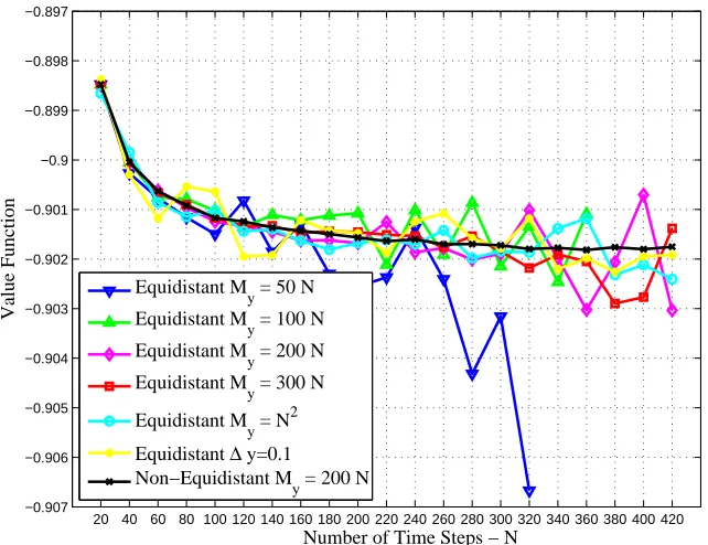
We also compare the performance of non-equidistant and equidistant dis-cretizations in the case of the state-dependent drift µL(t, S(t)). Figure 2
shows that the most stable results are obtained under the non-equidistant discretization. The precision of the approximation increases gradually as the number of time steps increases. Equidistant discretizations exhibit a more volatile behavior.
7
λ= 0.005 λ= 0.01 λ= 0.02 λ= 0.03
Monoyios [0.3866, 0.5780] [0.3499, 0.6197] [0.2702, 0.7196] [0.1813, 0.8243]
Equidistant [0.3870, 0.5772] [0.3510, 0.6193] [0.2708, 0.7137] [0.1851, 0.8161]
Non-equidistant [0.3864, 0.5763] [0.3527, 0.6209] [0.2720, 0.7177] [0.1826, 0.8113]
[image:21.612.86.531.126.228.2]Range of y [-10.748, 16.213] [-24.622, 30.443] [-56.800, 64.677] [-109.43, 128.71]
Table 1: Boundaries of no-trade region at t = 0. The first row is taken from
Monoyios (2004, Table 1) using a binomial lattice: r = 0.1, ∆t= 0.02,µ= 0.15,
σ = 0.25, S0 = 15, α = 0.1, T = 1 year. The second row uses the equidistant
discretization with ∆y = 0.0001, while the third row uses the non-equidistant
discretization (11) with My = 3,500 and ϖ = 1.6. The last row presents the
ranges of y grid determined by equations (A.2) and (A.5) inMonoyios (2004).
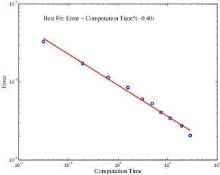
We finally consider the relationship between computation time and nu-merical accuracy. Figure 3 shows the log-log scale plot8 for the absolute error |Vi − Vˆ| of the value function V(t = 0, s = 15, x = 0, y = 0) and
computation time for the non-equidistant discretization with local search in the case of the state-dependent drift µL(t, S(t)). Specifically, the quantities Vi are the results using non-equidistant discretization and N = 20 +i×20, i = 0,1, . . . ,9, in Figure 2. The benchmark ˆV = −0.9018 is obtained by using non-equidistant discretization and N = 420 in Figure 2. We assume
ˆ
V is a reliable approximation of the true value of V(0,15,0,0). Then the difference |Vi − Vˆ| between Vi and the “true” value ˆV is the error of
nu-merical algorithm. An increase in N reduces the error at the cost of longer computation time, as shown in Figure 3.
8
20 40 60 80 100 120 140 160 180 200 220 240 260 280 300 320 340 360 380 400 420 −0.907
−0.906 −0.905 −0.904 −0.903 −0.902 −0.901 −0.9 −0.899 −0.898 −0.897
Number of Time Steps − N
Value Function
Equidistant My = 50 N Equidistant M
y = 100 N
Equidistant M
y = 200 N
Equidistant My = 300 N
Equidistant M
y = N 2
Equidistant ∆ y=0.1 Non−Equidistant M
[image:22.612.146.467.127.374.2]y = 200 N
Figure 2: Value functions at initial time versus the number of time stepsN with
the state-dependent driftµL(t, S(t)), whereN = 20+i×20,i= 0,1, . . . ,20. Other
parameters are the same as in the base case.
To estimate the order of time-complexity, we first assume the relationship
|V −Vˆ|=a τ−b, where τ is computation time and we call b the convergence
order. We estimate b (and loga) by performing an ordinary least squares regression of log(|V −Vˆ|) on log(τ).
All observations in Figure 3 are close to a straight line with slope −0.4 (taking logarithms of both variables). This means that to halve the numerical error, computing time is increased by a factor of 2(1/0.4) ≈5.7. Note that this
10−2 10−1 100 101 102 10−4
10−3 10−2
Computation Time
Error
[image:23.612.144.465.127.383.2]Best Fit: Error ~ Computation Time^(−0.40)
Figure 3: Convergence with non-equidistant discretization and the
state-dependent drift µL(t, S(t)). The y-axis reports the absolute error |Vi −Vˆ| of
the value function V(t = 0, s= 15, x= 0, y = 0). The benchmark ˆV = −0.9018
has been obtained by usingN = 420, andVi’s are the results withN = 20 +i×20,
i= 0,1, . . . ,9.
be halved) and much faster than for the direct method (8), where a simple halving of all step sizes increases computation time by a factor of 32. In Appendix A, we investigate the convergence order for different random sets of values of parameters9. This confirms the robustness of the results reported in Figure 3.
9
4. Results
The numerical solution technique is applied to study the effects of trans-action costs and uncertainty over investment time-horizons of up to 10 years. We consider the four types of investors introduced in Definition 2.1.
Our numerical results provide three main insights of practical relevance:
• Not knowing the true stock price dynamics leads to large losses in utility for less risk-averse investors, strongly biased investors, and naive investors (in decreasing order).
• Learning generally reduces the loss in utility caused by uncertainty about the true drift.
• Lower trading volumes due to transaction costs explain about half of the total loss in utility. The other half is caused by transaction cost payments.
a lower average realized utility than expected ex ante. We therefore take realized rather than perceived utility when measuring losses relative to an informed investor.
Section 4.1 considers the value of knowing the realization of the drift and the true stock price dynamics (’value of information’) and Section 4.2
analyzes the true (economic) cost of proportional transaction costs.
4.1. Value of information
For each investor type, the average realized utility is given by
R(x) := EµU¯µ(x) (12)
where x is the initial money endowment (the initial share is zero). Eµ
de-notes expectation with respect to µ which has the distribution N(µ0, γ0).
The realized utility ¯Uµ is determined by the realized stock price path, the
investor’s realized trading strategy (L, M), and the utility function U:
¯ Uµ=E
{
U(x(T) +y(T)S(T)) |(L, M)}.
The average realized utility cannot be higher than the expected one, i.e.
R(x)≤EµVµ(0, S0, x,0),
where Vµ(0, S0, x,0) is the value of expected utility for a given µ. For naive
and biased investors, the inequality will, in general, be strict as these investors make incorrect assumptions about the stock price dynamics. Therefore they overestimate their expected utility. However, an informed investor’s average realized utility satisfies
where VF
µ(0, S0, x,0) is the expected utility which the investor maximizes
under knowledge of the value of µ. For a learning investor, who always uses µ0 as prior for the drift estimate at the initial time, the average realized
utility is
RL(x) = VL(0, S0, x,0).
The monetary value of being informed rather than having to learn the true drift over time from observations is:
IEL(x) = sup{c≥0RL(x)≤RF(x−c)}. (13)
This is the maximum amount a learning investor can pay to obtain the true value of µ without being worse off can be interpreted as an information
equivalent (IE). If the realization of the randomly drawn drift could be
purchased then IEL(x) were the highest price a learning investor is willing to pay to be certain about the value µ. Since the utility function (5) is CARA, the measure defined in (13) is actually independent of the monetary endowment x.
As the value functions of these two investors satisfy (9), one finds
IEL = 1
αexp(−rT) log (
HL/EµHµF
) ,
where H is the reduced form value function. An approximation ˆHF of the
expected value EµHµF is calculated as follows:
1. Draw independently Mµ values from the distribution N(µ0, γ0).
3. Calculate
ˆ
HF = 1 Mµ
Mµ
∑
i
HµFi.
Similar to (13), we can calculate the monetary value of being an informed investor rather than a naive investor or a biased investor. One first needs to solve the optimization problem to determine trading strategies. Using these strategies one can determine realized utility in a Monte Carlo simulation.10 To obtain the average realized utility one has to repeat this procedure for many draws of µ. In addition, these calculations have to be carried out for different levels of parameters for comparative analysis. The efficient numer-ical method in Section 3 allows performing these simulations in a matter of hours.
Figure 4 depicts information equivalents for different levels of risk aver-sion and different investor types. The lowest values are obtained for a learn-ing investor. This confirms that empirical estimation of the drift uslearn-ing the Kalman-Bucy filter (3) is beneficial. The highest values are associated with aggressive trend-followers and contrarian investors while less aggressive ones have information equivalents close to that of the naive investor.
Information equivalents are decreasing in the risk aversionα: more risk-averse investors receive lower benefits from knowing the true drift. For in-stance, the investors with α= 0.5 are only willing to pay from about 17% to
10
We use Mµ = 1,001 during a simulation. Our results show that our sample
0.1 0.15 0.2 0.25 0.3 0.35 0.4 0.45 0.5 0
1 2 3 4 5 6 7
Absolute Risk Aversion Parameter − α
Information Equivalent
Mean Reversion a = 0.5 Trend−Follower a = − 2 Mean Reversion a = 0.1 Naive Investor
[image:28.612.147.466.128.387.2]Trend−Follower a = − 0.1 Trend−Follower a = − 0.4 Learning Investor
Figure 4: Information equivalents for different levels of risk aversion,T = 1 year.
25% as much as the investors with α= 0.1 to remove uncertainty about the actual drift. At first sight this might be surprising as higher risk-aversion is generally associated with higher willingness to pay in order to avoid risk. The opposite is true here as higher risk aversion leads to less investment in the stock, see also Muthuraman and Kumar (2006). Cvitani´c et al. (2006) also find that the certainty equivalents that they examine achieve the highest values for the lowest risk aversion in different setups.
−2 −1.5 −1 −0.7 −0.5 −0.3 −0.1 0 0.1 0.5 2.5
3 3.5 4 4.5 5 5.5 6 6.5
Sentiment Parameter − a
Information Equivalent
(a) IE versus sentiment parametera
1 2 3 4 5 6 7 8 9 10 0
0.5 1 1.5 2 2.5 3 3.5
Time Horizon − T (Year)
Annualized Information Equivalent
Naive Investor Learning Investor
[image:29.612.117.506.131.309.2](b) IE versus time horizonT
Figure 5: This figure illustrates information equivalents for: (a) biased investors
with different values of a(see (4)): naive investor (a= 0), trend-follower (a < 0)
and contrarian investor (a >0); and (b) different investment horizons.
investor therefore mimics the optimal filtering. Hence, the trading strategy of an investor whose estimate of the drift is derived from cautious interpolation of an observed short-term trend, is close to that of a learning investor.
The effect of the investment time-horizon T on the (annualized) infor-mation equivalent is studied in Figure 5(b), which is defined as IE·erT/T
hori-zon. The lesson is that the true drift is difficult to estimate and one cannot eliminate uncertainty about the drift. Thus, learning via filtering has benefits even in the long run. A naive investor with a 1-year (10-year) horizon could reduce the loss by 33% (80%) when adopting a filtering strategy. Previous studies using filtering without transaction costs also find substantial utility gains from 2.93% to 215.73%, see Cvitani´c et al. (2006).11
4.2. Transaction costs
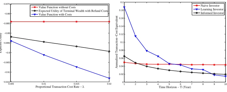
Trading strategies are sensitive to transaction costs. Figure 6(a) shows the utility of a learning investor under different scenarios. The top line is the benchmark case of no transaction costs. The bottom line is the utility with transaction costs, which is decreasing as the proportional transaction cost increases. This coincides with previous studies (see, e.g. Gennotte and Jung 1994). In the range 0.5% to 2% the loss in utility is approximately linear.
This loss is caused by two effects of transaction costs: (a) a direct ef-fect due to the additional expense incurred and (b) an indirect efef-fect due to less trading. We strip out the first one by reimbursing all transaction costs (with interest) at the final period. The investor optimizes his strategy without knowing about this reimbursement. The result is the middle line in Figure 6(a) which is about halfway (except those for the small λ < 0.01) between the zero-cost and positive-cost without reimbursement case.
The difference between the reimbursement and the zero-cost case is the deadweight loss from the transaction costs. It measures the true economic
11
0.005 0.01 0.015 0.02 −0.915 −0.91 −0.905 −0.9 −0.895 −0.89 −0.885 −0.88 −0.875
Proportional Transaction Cost Rate − λ
Expected Utility
Value Function without Costs
Expected Utility of Terminal Wealth with Refund Costs Value Function with Costs
(a) Expected utility with three cases of costs
1 2 3 4 5 6 7 8 9 10 0 0.02 0.04 0.06 0.08 0.1 0.12 0.14 0.16 0.18 0.2
Time Horizon − T (Year)
Annualized Transaction−Cost Equivalent
Naive Investor Learning Investor Informed Investor
[image:31.612.118.506.131.288.2](b) TE versus time horizonT
Figure 6: This figure depicts (a) maximum expected utility of a learning investor
under three situations of transaction costs; and (b) transaction-cost equivalents of
naive / learning / informed investors within different investment horizons.
cost of this friction. We find that the total effect of the transaction cost is about twice (except λ < 0.01) as large as the loss in utility due to less trading resulting from transaction costs. The implications are that freely re-balancing portfolio significantly contributes to expected utilities, and less re-balancing brings about half of the total loss.
To capture the value from investing in a market without transaction costs, we denote the gain to an investor of type · as
TE·(λ) = sup{c≥0E
µVµ,λ· (0, S0, x,0)≤EµVµ,λ· =0(0, S0, x−c,0)}, (14)
where V·
µ,λ(0, S0, x,0) is the value of expected utility. In contrast to IE in
will-ing to pay to avoid transaction costs. The CARA utility function (5) implies that the measure is independent of the monetary endowmentx. AsV satisfies (9), one has
TE·(λ) = 1
αexp(−rT) log (
EµHµ,λ· /EµHµ,λ· =0
) .
We express TE·(λ) in a consistent way withµ as one of the subscripts in H without specifying an investor. In fact, only for an informed investor, does the value function depend on µ ∼ N(µ0, γ0). For all other types, one can
drop Eµ and the subscript µ.
Figure6(b) shows the welfare effect of transaction costs on three investor types. The annualized transaction-cost equivalents are approximately con-stant for the naive investor but slowly decreasing for the informed investor and rapidly decreasing for the learning investor. For time-horizons of up to 5 years, the learning investor is the one most strongly affected because the estimate of the drift is inaccurate and can vary drastically in the short run (e.g. Lundtofte 2008).12 This increases the learning investor’s incentive to trade and leads to higher transaction costs.
At longer time horizons, the naive investor has the most to gain from the absence of transaction costs as the misspecification of the drift leads to excess trading compared to the investors who either know or have learned enough about the actual drift. For a learning investor, trading is slightly contrarian, which leads to the lowest transaction-cost equivalent. For instance, a sudden sharp drop (rise) in the stock price leads to a stock purchase (sale) from the
12
informed investor. A learning investor at the same time lowers (increases) the estimate of the drift and therefore tends to make a smaller trade, incurring lower transaction costs. As a result, the learning investor reduces the loss in utility by about 50% over a 10-year time-horizon compared with the naive investor. The benefit of learning mirrors the substantial utility gains found
by Cvitani´c et al.(2006) without considering transaction costs.
5. Conclusion
The efficient algorithm introduced in the paper allows us to solve portfo-lio optimization problems with state-dependent drift and long time-horizons in the presence of proportional transaction costs. We apply the method to explore scenarios in which investors (a) use past stock prices to learn about the true drift, (b) react to stock price movements as trend-followers or con-trarians, or (c) are naive and ignore information revealed over time.
The numerical results show that forecasting behavior has a strong impact on trading. We quantify the value of information and the welfare effect of transaction costs. Information is most valuable to the least risk-averse in-vestor, and transaction costs are most detrimental to naive investors. The total loss in utility from transaction costs is generally about twice as large as the direct cost incurred. Learning reduces the utility losses due to the un-certain drift and transaction costs, especially for medium and long horizons.
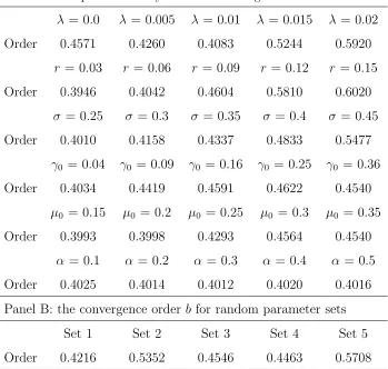
Appendix A Test of Convergence Order
Panel A: comparative analysis of the convergence order b
λ = 0.0 λ = 0.005 λ = 0.01 λ = 0.015 λ = 0.02 Order 0.4571 0.4260 0.4083 0.5244 0.5920
r = 0.03 r = 0.06 r = 0.09 r = 0.12 r = 0.15 Order 0.3946 0.4042 0.4604 0.5810 0.6020
σ = 0.25 σ = 0.3 σ = 0.35 σ = 0.4 σ = 0.45 Order 0.4010 0.4158 0.4337 0.4833 0.5477
γ0 = 0.04 γ0 = 0.09 γ0 = 0.16 γ0 = 0.25 γ0 = 0.36
Order 0.4034 0.4419 0.4591 0.4622 0.4540 µ0 = 0.15 µ0 = 0.2 µ0 = 0.25 µ0 = 0.3 µ0 = 0.35
Order 0.3993 0.3998 0.4293 0.4564 0.4540 α = 0.1 α = 0.2 α = 0.3 α = 0.4 α = 0.5 Order 0.4025 0.4014 0.4012 0.4020 0.4016 Panel B: the convergence order b for random parameter sets
Set 1 Set 2 Set 3 Set 4 Set 5
[image:34.612.132.481.175.507.2]Order 0.4216 0.5352 0.4546 0.4463 0.5708
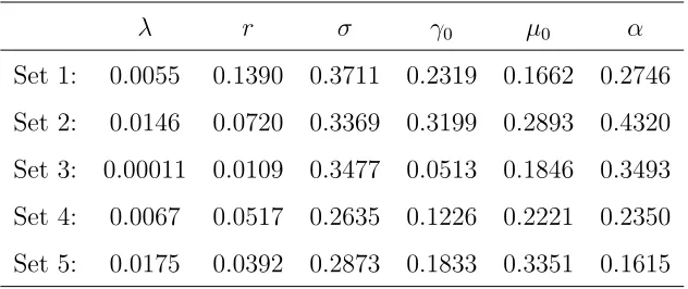
Table 2: This table displays the convergence order b with non-equidistant
dis-cretization and the state-dependent drift µL(t, S(t)). Panel A shows the
compar-ative analysis of bto six parameters. Other parameters are the same as the base
case in Section3. Panel B lists the convergence order for five random sets of values
of parameters in Table3, assuming each parameter satisfies a continuous uniform
λ r σ γ0 µ0 α
[image:35.612.148.464.125.258.2]Set 1: 0.0055 0.1390 0.3711 0.2319 0.1662 0.2746 Set 2: 0.0146 0.0720 0.3369 0.3199 0.2893 0.4320 Set 3: 0.00011 0.0109 0.3477 0.0513 0.1846 0.3493 Set 4: 0.0067 0.0517 0.2635 0.1226 0.2221 0.2350 Set 5: 0.0175 0.0392 0.2873 0.1833 0.3351 0.1615
Table 3: The random sets of values of parameters.
that for the state-dependent drift, the computing time of our algorithm is increased by a factor of 2(1/0.4) ≈ 5.7 in order to halve the numerical error.
Here we test the convergence orderbfor different sets of values of parameters. In general, the test results show that the convergence order b is at least around 0.4. In fact, it is faster for the most values of parameters tested. The speed of convergence is mainly affected by volatile no-trade regions of stock holdings due to our local search along with other improvements. Since we appropriately enlarge the no-trade regions of the successive nodes as the range of local search, we can locate the no-trade region faster if these regions do not change dramatically between adjacent nodes.
instance, a large risk-free r (a less attractive stock) or a large volatility σ (a riskier stock) implies substantially narrow and low no-trade region, which reduces computation time. In addition, the order slightly fluctuates around 0.40 to 0.46 for another three parameters since merely varying one of these values does not significantly change the volatility of the no-trade region.
References
Bj¨ork, T., Davis, M., Land´en, C., 2010. Optimal investment under partial information. Mathematical Methods of Operations Research 71, 371–399.
Brennan, M. J., 1998. The role of learning in dynamic portfolio allocations. European Finance Review 1, 295–306.
Clewlow, L., Hodges, S., 1997. Optimal delta-hedging under transactions costs. Journal of Economic Dynamics and Control 21, 1353–1376.
Cox, J. C., Ross, S. A., Rubinstein, M., 1979. Option pricing: A simplified approach. Journal of Financial Economics 7, 229–263.
Cvitani´c, J., Lazrak, A., Martellini, L., Zapatero, F., 2006. Dynamic portfolio choice with parameter uncertainty and the economic value of analysts’ recommendations. Review of Financial Studies 19, 1113–1156.
Davis, M. H. A., Panas, V. G., Zariphopoulou, T., 1993. European option pricing with transaction costs. SIAM Journal on Control and Optimization 31, 470–493.
Gennotte, G., Jung, A., 1994. Investment strategies under transaction costs: The finite-horizon case. Management Science 40, 385–404.
Glasserman, P., 2004. Monte Carlo Methods in Financial Engineering. Springer, New York.
Herzog, R., Kunisch, K., Sass, J., 2013. Primal-dual methods for the compu-tation of trading regions under proportional transaction costs. Mathemat-ical Methods of Operations Research 77, 101–130.
Kushner, H., Dupuis, P., 1992. Numerical Methods for Stochastic Control Problems in Continuous Time. Springer, New York.
Lensberg, T., Schenk-Hopp´e, K. R., 2013. Hedging without sweat: a genetic programming approach. Quantitative Finance Letters 1, 41–46.
Luderer, B., Nollau, V., Vetters, K., 2010. Mathematical Formulas for E-conomists, 4th Edition. Springer, New York.
Lundtofte, F., 2008. Expected life-time utility and hedging demands in a partially observable economy. European Economic Review 52, 1072–1096.
Monoyios, M., 2004. Option pricing with transaction costs using a Markov chain approximation. Journal of Economic Dynamics and Control 28, 889– 913.
Muthuraman, K., Kumar, S., 2006. Multidimensional portfolio optimization with proportional transaction costs. Mathematical Finance 16, 301–335.
Shefrin, H., 2008. A Behavioral Approach to Asset Pricing Theory, 2nd Edi-tion. Academic Press, San Diego.
Wang, H., 2010. Optimal Portfolio Choice under Partial Informa-tion and TransacInforma-tion Costs. PhD thesis, University of Leeds, http://ssrn.com/abstract=1664427.