Adaptive signal processing techniques to detect time varying late potentials on a beat to beat basis

1-1-1995

Adaptive signal processing techniques to detect

time-varying late potentials on a beat-to-beat basis

Subbaraman Narayan

Iowa State University

Follow this and additional works at:https://lib.dr.iastate.edu/rtd Part of theEngineering Commons

This Thesis is brought to you for free and open access by the Iowa State University Capstones, Theses and Dissertations at Iowa State University Digital Repository. It has been accepted for inclusion in Retrospective Theses and Dissertations by an authorized administrator of Iowa State University Digital Repository. For more information, please [email protected].

Recommended Citation

Narayan, Subbaraman, "Adaptive signal processing techniques to detect time-varying late potentials on a beat-to-beat basis" (1995). Retrospective Theses and Dissertations. 18565.

by

Subbaraman Narayan

A Thesis Submitted to the

Graduate Faculty in Partial Fulfillment of the

Requirements for the Degree of

MASTER OF SCIENCE

Departments: Biomedical Engineering

Electrical and Computer Engineering Co-Majors: Biomedical Engineering

Electrical Engineering

Signatures have been redacted for privacy

Iowa State University Ames, Iowa

TABLE OF CONTENTS

CHAPTER 1. INTRODUCTION

1.1 Overview . ... . . ... . 1.2 Clinical Significance of Late Potentials 1.3 Need for the Study . . .

1.4 Origin of Late Potentials 1.5 Mechanism of Late Potentials 1.6 Signal Characteristics . . . . 1.7 Summary of Previous Work 1.8 Scope of This T hesis . . . .

1 1 2 3 4 4 5 6 8

CHAPTER 2. HIGH RESOLUTION ELECTROCARDIOGRAPHY 10

2.1 Introduction . . . . 2.2 Technical Aspects of Signal Averaged ECG System

2.2. l Electrodes 2.2.2 Hardware 2.3 Signal Averaging

2.3. l Time Domain Analysis

2.4 Beat to Beat Analysis of ECG signals .

2.4.1 Disadvantages of the Signal Averaged ECG System

2.4.2 Statistics of the ECG Signal

2.-1.3 ~1ethods of Noise Reduction

2.4.4 Quantification of Noise 2.5 Proposed System ... .

CHAPTER 3. ADAPTIVE NOISE CANCELER

3 .1 Introduction . . . . 3.2 Principle of a Correlator Canceler 3.3 L:\1S and the Leaky LMS . ....

CHAPTER 4. DYNAivlIC TIME WARPING

4.1 Introduction . . . . 4.2 Warping Principle .

4.2.1 Restrictions of the Warping Function 4.2.2 Weighting coefficient . . .

4.3 Practical DP matching Algorithm

4.3. l DP equation .

4.3.2 Calculation .

CHAPTER 5. TIME - SEQUENCED ADAPTIVE FILTER

5.1 Introduction ... 5.2 TSAF algorithm .

5.2. l Filter Description .

5.2.2 Disadvantages of the TSAF 5.2.3 Typical Applications . . . .

5.3 Proposed Scheme to Detect Late Potentials .

CHAPTER 6. SIMULATION RESULTS

..

6.2 Simulation methods .

6.2.1

6.2.2

6.3 Dynamic Time Warping

. ....

6.4 Modeling Late Potentials .

.. ....

CHAPTER 7. CONCLUSIONS

BIBLIOGRAPHY

... .

51 51 53 53

54

62

67

67

70

Figure 1.1

Figure 1.2

Figure 2. 1

Figure 2.2 Figure 2.3 Figure 2.4 Figure 2.5 Figure 2.6 Figure 2.7 Figure 3.1 Figure 3.2 Figure 4.1 Figure 4.2 Figure 4.3 Figure 5.1 Figure 5.2 Figure 5.3 Figure 6.1

LIST OF FIGURES

The Infarcted Heart ... ... ... 6

A Typical X Lead Waveform ... 7

The Signal Average ECG System ... ... 11

XYZ Electrode Placement Scheme ... ... 12

Root Mean Square Value ... ... ... 15

RR Interval Variability and RR Detection ... ... 16

The Differences in two QRS Beats ... ... ... 18

Calculation of Noise Figure ... ... 22

Proposed Real Time System ... 23

Correlator Canceler ... 26

The Leaky LMS ... ... ... ... 27

The Warping Function ... ... 32

The Different Warping Algorithms ... 37

Flow Chart for DTW ... 41

Symbolic Representation ... : ... 43

Time Varying Error Surface ... ... 45

Proposed TSAF to Detect Late Potentials ... ... 50

Figure 6.2 Time Averaging ... ... ... .. ... 53

Figure 6.3 The Orthogonal Leads and the Corresponding Butterworth Filtered Outputs ... ... ... 55

Figure 6.4 The X Lead: Raw X Lead, Output of LMS Based Adaptive Filter and the Output of the Leaky LMS Based Adaptive Filter. ... 56

Figure 6.5 The Y Lead: Raw Y Lead, Output of LMS Based Adaptive Filter and the Output of the Leaky LMS Based Adaptive Filter.. ... 57

Figure 6.6 The Y Lead: Raw Y Lead, Output of LMS Based Adaptive Filter and the Output of the Leaky LMS Based Adaptive Filter. ... 58

Figure 6.7 RMS Value Comparison Before and After Adaptive Filtering ... ... 59

Figure 6.8 The Beat-to-Beat Estimate of the RMS Value After Adpative Filtering ... 60

Figure 6.9 Comparison of Noise Figures for Different Time Lengths and Comparison in the Performance of the Exisiting Technique to the Adaptive Filtering Technique ... ... ... ... 61

Figure 6.10 Case 1: The Peaks are not Aligned ... ... 64

Figure 6.11 Case2: The Peaks are Aligned and then Warped ... ... 65

Figure 6.12 The Effects of Warping ... ... ... ... 66

Figure 6.13 Model of Late Potentials ... ... ... ... 68

ACKNOWLEDGl\tlENTS

I am deeply indebted to my major professor, Dr. John F. Doherty, for giving me valuable advice, encouragement and making critical reviews on my work. I would also like to thank him for making my stay at Iowa State a memorable and pleasant one. I would like to thank my major professor, Dr. Robert Weber, for his patience and support in the course of my work. I would also like to thank Dr. Allison Flatau who helped me to get through my thesis without any financial burden and for the time she took to serve on my committee.

I would like to thank Mr. Jian Huang for his valuable help to code the programs in assembly language and spending long hours in the lab helping me to solve a lot of software problems. I would like to thank Mr. Hal Gant, Del Mar Avionics for the valuable XYZ data. I would also like to thank Dr. Cameron Spiers, University of Strathclyde for his valuable advice regarding this work.

CHAPTER 1. INTRODUCTION

1.1 Overv iew

Ventricular late potentials are low amplitude, high frequency signals present in the terminal portion of the QRS of an ECG signal. These fragmented potentials are caused by the abrupt termination of the activation waveform in the electrically silent infarcted region. The non-invasive detection of these microvolt signals was first reported in 1973 [1] by using high gain amplification and ensemble signal averaging. Recent studies show that the presence of ventricular tachycardia (VT) can be quan-tified using late potentials [2). It is an accepted indicator for identifying patients at risk for life threatening arrhythmias. A system which monitors these signals has a potential application in screening patients who are susceptible to various kinds of arrhythmias. Berbari was the first to demonstrate the feasibility of recording VLP's

from the body surface signals [3]. He also showed a correspondence between the sur-face recorded signal and those signals recorded directly from the epicardial sursur-face. As late potentials are small in comparison with the amplitude of the QRS complex,

the conventional ECG is unable to detect these signals. The signal averaged electro-cardiogram (SAECG) has become a widely accepted technique for risk stratification of patients. The SAECG primarily uses two signal processing techniques to process

However there are several potential disadvantages of signal averaging. This technique cannot detect any beat-to-beat variations. This thesis presents a real time system

to detect the late potentials on a beat-to-beat basis allowing assessment of dynamic changes in these signals that occur after drug therapy. The Leaky LMS algorithm is used for the enhancement of late potentials. The system is realized using a Motorola 56001 (DSP P rocessor). Approximately 13,000 instructions can be performed at a rate of 1 sample per millisecond. The commercially available SAECG devices average anywhere between 250-300 cycles to reduce the noise to approximately 1 microvolt. Thus at a sampling rate of lOOOHz and each QRS beat almost a second this corre-sponds to 4-5 minutes before the RMS values can be determined. The DSP based SAECG algorithm can be used to generate RMS values in seconds and is easily incor-porated to a stand alone system. Dynamic time warping is investigated for coherent averaging. The time varying filter is also discussed as an alterative to the SAECG system.

1.2 Clinical Significance of Late Pot ent ials

infarc-ti on who may be at risk of sudden death. Studies by Dennis, et.al. , showed that 903 of the patients (survivors of acute myocardial infarction) who subsequently de-veloped VT had persistence of late potentials [2]. Late potentials are the signals produced during the polarization of damaged ventricular tissue. Studies have shown a correlation between late potentials and fibrillation which have made this a marker for identifying patients with life threatening arrhythmias [2].

1.3 Need for the Study

The SAECG has become a widely accepted technique for risk stratification of patients with potential reentrant arrhythmias. Presently six devices are commer-cially available in the United States for identification of late potentials. All these

devices analyze the ECG by Simson's method [4]. They all employ a signal averag-ing algorithm. Although these devices employ a generally similar approach, totally standardized methods and criteria for the detection of late potentials have not yet

been developed [2]. The results obtained from signal averaging depend on the align-ment of the signals to be averaged. The average predictive accuracy is about 643 [5]. This technique does not allow the detection of dynamic changes in ventricular

late potentials which may occur either spontaneously or during various diagnostic and therapeutic interventions. The clinical advantage of detecting late potentials on a beat-to-beat basis is that it facilitates the study of the relationship between late

1.4 Origin of Late Potentials

Late potentials are usually found in the border zones surrounding the scar of a previous myocardial infarction [6]. The border zone that exists between scar tissue and normal tissue is composed of conducting and non-conducting tissue. Interstitial fibrosis forms in the insulating boundaries and this results in slowing and fragmen-tation of the wave of electrical depolarization. Therefore the border zone is both the source of late potentials and the substrate for re-entrant ventricular tachycardia.

1.5 Mechanism of Late Potentials

The delayed conduction that manifests itself as a 'late potential' can be caused primarily by one of two factors: slow conduction velocity or a long path length of conduction. Slow conduction velocity can be due to depressed membrane characteris-tics, or changes in anisotropic conduction properties caused by increased cell coupling

resistances, or both. Conversely, the long path length of conduction is prolonged by tortuous conduction around regions of anatomical or functional conduction blockage. Infrequently, there is yet a third factor that can cause late potentials. Although most late potentials have been associated with depolarization of cardiac tissue,

and Slow cond uction. In Figure 1.1 we observe that when an impulse traversing the tissue encounters the proximal end (A, Figure 1.1) of the area of decremental conduction, where antegrade conduction is blocked, the normal propagation of the

impulse through the myocardium continues and the impulse is eventually conducted to a point beyond the area of decremental conduction. At t his point the impulse enters the depressed area from its distal end (B), and because t he block is only in the antegrade direction the impulse is able to pass through the area of decremen-tal conduction in a retrograde direction, emerging after a delay at the proximal end

(A). If the impulse has been sufficiently delayed in its passage through t he area of

decremental conduction, it arrives(re-enters) (A) after the normal tissue proximal to the depressed area has been recovered. In this way the second impulse is initiated in the proximal region of the myocardium that is propagated as a premature excitation. This excitation may in turn cause another excitation and through repetition of this mechanism, a run of premature excitations causes tachycardia.

1.6 Signal C haracteristics

Late potentials are identified as low amplitude, high frequency signals which are continuous with the QRS complex and extend to the ST segment. The signal is

typically characterized as being between 1 - 40µvolts and comprised of frequencies

Area of Decremental Conduction

I 2

~

t

I 2

Figure 1.1: The Infarcted Heart

1.7 Summary of Previous Work

p

R

~

~ QRS ~

: Duratibn

Late Potentials

T

--- ---·---()-6 _____ _

₀

0.2

0.4

.

Time (s)

Figure 1.2: A Typical X Lead ECG Waveform

synthesis was done by Tuteur in [14]. Tuteur modeled late potentials as a sine wave modulated by a gaussian envelope and he applied wavelets transformations to

de-tect t hese synthesized late potentials. Autoregressive modeling was done by Lander, et.al, [15] to detect intra-QRS late potentials. Spectrotemporal maps and frequency domain analysis using autoregressive modeling was perfected by Chan [16]. These

met hods are now applied real time in commercial devices to detect late potentials using spectrotemporal maps. Statistical methods like the maximum likelihood

es-timator were used to detect late potentials by Attarinejad [17]. Cameron,et.al, [8]

per-formed bispectral analysis. Detection of a late potentials using adaptive filters was first suggested by Al-Nashash [18] and \.Vang [19]. Shelton and Coast also proposed detection of late potentials by adaptive filtering [20]. Recursive least squares filtering was suggested by Cameron [21] and the time variant filter was suggested by Coast [20] . Both [20, 21] showed results for synthesized late potential's. It was however observed that late potential's have not been modeled successfully in literature. The recent method for detection of late potentials was suggested by Chen [22] using P rony's method. Most researchers who applied different feature extraction techniques like wavelet transforms or Prony's method or other statistical estimators have used the averaged electrocardiogram. The question arises whether any variable late potentials have been lost.

1.8 Scope of T his Thesis

The signal averaged ECG primarily uses two signal processing techniques to process the cardiac signal for late potential analysis: time ensemble averaging; and filtering. The standard technique for detection of VLP's results in a time-domain vector magnitude time series formed from a signal averaged, high pass filtered, three lead data set. The averaging technique can only detect late potentials which are ab-solutely constant in duration, morphology, and timing with respect to the QRS com-plex. Therefore, this technique cannot detect any beat-to-beat variations. Recording of late potentials on a beat-to-beat basis has the potential of directly identifying reentrant 'malignant' versus focal 'benign' ventricular rhythms [2, 23]. Researchers found that spatial averaging is an alternative to the time average. But spatial

thesis techniques to detect late potentials real time using adaptive filters is described.

CHAPTER 2. HIGH RESOLUTION ELECTROCARDIOGRAPHY

2.1 Introduction

Ambulatory electrocardiography is recognized as a valuable non-invasive cardio-logic diagnostic test to asses changes of cardiac arrhythmias and heart rate variability

[11]. It has been observed that this scheme is not suitable to detect high frequency

cardiac depolarizations. High resolution electrocardiography is the technique that is used to enhance the detection of low amplitude signals. The hardware used in this technique is described in the following section. The signal averaged ECG system is shown below in Figure 2. 2.

2.2 Technical Aspects of Signal Averaged ECG System

The standards for the hardware are defined in [24]. Commercially available devices comply with this standard.

2.2.1 Electrodes

Real-time signal averaging utilizes three orthogonal bipolar leads X Y and Z

to record the cardiac electrical activity from the body surface. For recording late

potentials from the surface of the body, most investigators use an XY Z lead system

Y Leads

Figure 2.1: XYZ Electrode Placement Scheme

X lead is placed at the fourth intercostal space in both midaxillary lines. The Y lead should be positioned on the superior aspect of the manubrium and on either

the upper left leg or left iliac crest. The Z lead should be positioned at the fourth

intercostal space

(V2)

impedance should be less than lOOOn.

2.2.2 Hardware

The typical hardware is shown in Figure 2.2. The ECG signal obtained from the

orthogonal leads is amplified and the data is sampled at 1000 Hz. The A/D converter

y.

z

X-Z+

Amplifier X+

--...

Signal Averaging Technique

AID Converter

_____...

_.

\ ,

Filtering

.__

Template Recognition

D

summed Lists Cardiac Cycles

matching and alignment of the accepted QRS complexes. Time domain analysis is done using the Simson's method. The beats after alignment and smnmation are passed through a bi-directional four pole Butterworth filter as recommended by the American College of Cardiology (ACC) policy statement [24]. Ringing effects of high pass filtering may prevent proper quantification of late potentials. Simson [4] adopted a variant of bi-directional filtering. The data is filtered roughly until the mid point of the QRS and then stops filtering which allows the ringing to subside before the end of the unfiltered QRS. The data is then reverse filtered through the same point until the QRS mid point. The filter has a bandpass 40-250 Hz or 20-250 Hz. Results are based on analysis of the vector magnitude of the filtered leads that is known as the

RMS value and is defined

JX

+

+

QRS duration is then verified visually by the technician.

2.3 Signal Averaging

These standards indicate that the noise should be less than lmV with a 25 Hz

high pass or less than 0.7µV with a 40 Hz cut off when used with the combined vector

magnitude of XY Z leads. The first step is to find a reference point. For this purpose

the R wave is usually selected. After this, beats are aligned and averaged. The

computer algorithm should be capable of excluding ectopic (noisy) beats. Testing of new beats should be performed across all input leads. Mostly a cross-correlation is used for template matching and a correlation greater than 98% is used for acceptance.

Beats are accepted for averaging only if the

R

R

2.3.1 Time Domain Analysis

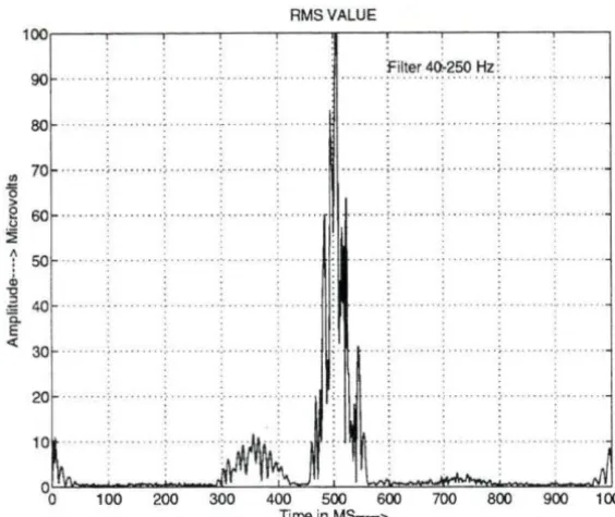
Results of most studies have been based on the analysis of the vector magnitude of the filtered QRS complex. The filtered QRS duration, RMS amplitude of the

ter-minal 40msec of the QRS complex, and the low amplitude signal duration measured

from the QRS endpoint until the signal exceeds 40µ V are the parameters needed

to establish the presence of fragmented potentials (Figure 2.3). The filtered QRS

complex is defined as the midpoint of a 5msec segment in which the mean voltage

exceeds the mean noise level plus three times the standard deviation of the noise sample [2]. The endpoint of the QRS complex should be verified visually and the system allows manual adjustment of the automatically determined end points. The definition of a late potential and the scoring of a high resolution ECG as normal or abnormal have not yet been standardized [24]. Representative criteria include that a late potential exists (using 40 Hz high pass bi-directional filtering) when

1. The filtered duration of the QRS complex is greater than l 14msec.

2. There is less than 20µ V of signal in the last 40msec of the vector magnitude

complex, and

3. The terminal vector magnitude complex remains below 40µ V for more than

RMS VALUE

l=ilter 40-250 Hz

90 .... ... . . ... ... .. ... ..

80 ... •... . ... ~.. . .. . . '. . . . .

.

"' 70

-15 _>

§ 60

~

i

.,

~ 40 Ci.

E

<t 30

... ; ... ; ... .

... 1 . . . 1 . . . .

... . . . . . . .. . . .. .. . .... . .. . ... .. .. . ···-·· ... _. , ... _. ,,. _. . ... ... ... .. . _{. . .} . . .

20 ···'·· ···: _. ... ···:--···: ... _{. .} ····:···:··· .... ····:···· ...

. . .

. . .

10

0_{o 100 200 300 400 500 600 700 800 900 1000}

Time in MS-->

Figure 2.3: Root Mean Square Value

2.4 Beat to Beat Analysis of ECG signals

2.4.1 Disadvantages of the Signal Averaged ECG System

Signal averaging techniques has many disadvantages. The two major limitations are that it will not be able to detect dynamic (beat-to-beat) changes in the signal due to sinusrhythm; and the SAECG cannot be recorded during complex cardiac

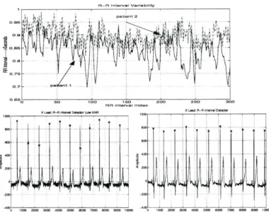
arrhythmias. The variability of the R-R intervals is seen in Figure 2.4. The QRS

detection algorithms [25) perform poorly under low SNR conditions. This is

A - A tnturval Varlablllty

!E 0 . 75

o .7

0·85o!---=so'=---,, o~o,..---,,~so=---=2~000:---::2:-::so::---;;;300

RR lnto""al lndOJC

-

-

- 200

Figure 2.4: RR Interval Variability and RR Detection

low SNR environment and the other shows the performance of the algorithm under a

high SNR. Even ±3msec error in detection of peaks may cause a significant change

in the quantification of late potentials.

the assumption that the late potentials are constant in timing relative to the QRS. Another asswnption is that the late potentials are fixed in both morphology and duration. These are poor assumptions as the late potentials are influenced by factors like the nature of the infarct and the time or the number of days after the infarct [6]. Since late potentials originate from ischemic areas where physiologic conditions are unstable, they are inherently variable in terms of amplitude, bandwidth, and timing within the cardiac cycle (23]. The variability of late potentials are compounded by variations in the heart rate in Figure 2.4. Variations in heart rate as small as

20% can shift the activation patterns on ischemic ventricles by as much as lOmsec.

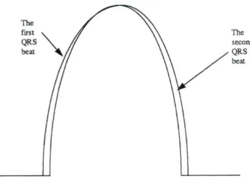
The results obtained from signal averaging also depend on the alignment of the beats. The QRS detectors have to be very precise else the QRS may manifest as a late potential. Probably the most important and best known source of beat-to-beat variability in cardiac electrical signals is respiration. Expansion of the thorax during inspiration produces two effects on the ECG. First, it induces a direct baseline shift mainly as a result of electrode impedance change and, second, it alters the electrical propagation of electrical signals from the heart to the body surface. Both artifacts can introduce significant timing errors and need to be considered. A study (23] showed that the most prominent influence on the orthogonal leads were on the QRS amplitude and azimuth. During deep inspiration, the QRS amplitude declined by 25% and azimuth increased significantly (in 69 patients) by an average of 11°. Respiration thus adversely influences the ability to align successive QRS complexes and determine the fiducial points. The effect of respiration was shown by simulating the ECG with a sinusoidal equation [23].

The second

QRS

bear.

Figure 2.5: The Differences in Two QRS Beats

Two QRS beats are shown above in Figure 2.5. As can be seen, perfect alignment of these complexes is not possible and hence any method including cross correlation will accumulate errors.

2.4.2 Statistics of the ECG Signal

The ECG signal contains noise components that can be traced to patient related origins, e.g., muscular activity and to the electronics of the recording equipment. Knowledge of the statistics of the noise is important to calculate the QRS endpoints

are power frequency, electrode-skin interface, amplifier noise and electromyogram (EMG) signals. The noise is a sswned to be uncorrelated with the ECG. However low frequency noise due to respiration may have a beat-to-beat correlation, which is removed by high pass filtering [18].

2.4.3 Metho ds of Noise R eduction

1. Signal Averaging

Signal averaging is analogous t o low pass filtering. The signal averager may be

viewed as a comb filter. The improvement in signal to noise ratio (SNR: defined as

the ratio of the signal power to the noise power) varies as

JFl

of averages. Consider adding together N beats and forming a mean beat or signal

average x(i). This is given as

N

L

Xj(i)

A ( " ) j=l

xi =

-N

(2.1)

where

Xj(i)

components can thought of as taking place independently that is

N N

2:

s1(i)

2:

ni(i)

x(i) = 1=1N

+

(2.2)

N

Since the cardiac signal is assumed to be identical,

L

(i)/N

j= l

(2.3)

hence the signal average is

x(i)

s(i)

+

~

(2.4)

2. Ensemble Averaging

Researchers studied spatial averaging as a method to improve the SNR [13].

Significant improvement in the SNR was observed in comparison with the signal averaging technique. The major advantage of spatial averaging is that it allows appreciation on a beat-to-beat basis of changing R-R intervals and other dynamic

changes in the heart. As spatial averaging requires averaging only two channels, the noise level in the vector magnitude was still high. There are many limitations to the spatial averaging technique. This technique is limited by the number of leads that

can be placed on the chest. It is difficult to find a good lead position. The EMG

noise in the parallel channels is not completely uncorrelated with each other and it is difficult to determine what the best positions are for the placement of the electrodes.

2.4.4 Quantification of Noise

The literature shows inconsistencies for quantification of noise. The definition used in this work is adapted from [2] and [23]. The noise measure is calculated by

selecting a signal free portion of the ECG signal that is in the later portion of the ST

segment, in the XY Z leads. The statistics of the noise was evaluated by calculating

lOOmsec afterwards). It was observed that histograms closely approximate a gaussian

distribution with a zero mean and a standard deviation between 10 - 20µ Volts.

Simulations were carried out for different sets of ECG signals and for different leads. The mean value was subtracted in order to reduce the effect of the signal component

when calculating the amplitude histograms. This technique was adapted from [27]. The assumption that the noise is gaussian is valid and the noise figure is calculated with those assumptions. A range of time windows for calculating the noise figure

(N.F) was seen in the literature [23]. Noise in t he three leads have different variances and closely approximate a gaussian distribution. Hence the vector magnitude is the sum of three non-central chi square distributions, resulting from the absolute value

operation performed on each lead. The N.F suggested in the literature for a good estimate [23] is defined as

l 3 m

3m

I: I:

(J'Jv

j = l k=l

NF= (2.5)

where j indicates the lead X , Y, Z and m equals the number of points in each lead

from which the noise is calculated. The N.F given in (2.5) is the average of the signal

variance for

m

leads.

The square root of N.F is the standard deviation of the noise process. Dividing

the N .F by

.Jii,

of the noise is observed in Figure 2.6 as a function of t he number of averages. A

lOmsec ·window was used to estimate N.F. For a variety of reasons, some ECG signals

Noise Figure

0.9 ... ... ... , ... , ...•.

0.8

ll

"fl

=

~

5

~ 0.6

~

=

>.

::n

j)

5

ll

::n

~ 0.3

>

~

0.2

0.1

···:··· ···:·· _. . ··· ·;· ... :·

···=-··· ,. . . 1•• •• •

. .. .. -:··· .. ·:· .. . ... . .. .

1

o

...

.

..

o l__~_i_==~=====r====::r:=====i====:::d

100 150 200 250 300 50

No of Averages

Figure 2.6: Calculation of Noise Figure

measure. Averaging to a noise factor of < 0.3µV is required for the accurate detection

of late potentials.

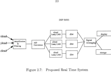
2.5 Proposed System

xlea zlea Amplification

n---

Lcalcy LMS

ylcad

Leaky LMS

zlead

Lcalcy L\1.S

Signal Averagin

Proposed Real Time System

commercial devices that exists run on the Motorola 68K processor working as fast as 27K instructions per second. Thus this system is limited in speed. The commercially available SAECG devices average anywhere between 250-300 cycles to reduce the

noise to approximately < 0.3µVolts. Thus at a sampling rate of 1000 Hz and each

Dynamic time warping is a technique used to align speech signals which differ due to speaking rate variation. This technique is used if time averaging of the beats is needed when the SNR from beat-to-beat is low. This is done to achieve a coherent

averaging scheme. Noise figures in the latter 10 - llOmsec of the ST segments were

calculated and a comparison was made with the existing averaging techniques. T he results show that the adaptive filtering enhancement of the low level cardiac signals on a beat-to-beat basis is significant. Other techniques like least squares filtering and

CHAPTER 3. ADAPTIVE NOISE CANCELER

3.1 Introduction

The usual method of estimating a signal corrupted by additive noise is to pass

the composite signal through a filter that tends to suppress the noise while leaving the signal relatively unchanged. Filters used for this purpose can be fL"Ced or adaptive. The design of fixed filters must be based on priori knowledge of both the signal

and the noise, but adaptive filters have the ability to adjust their own parameters automatically, and their design requires little or no prior knowledge of signal and noise characteristics. Noise cancellation is a variation of optimal filtering that is highly

advantageous in many applications. It uses an auxiliary or reference input containing

both signal and noise. As a result, the primary noise is attenuated or eliminated by cancellation. Adaptive noise cancellation was successfully applied to cancelling 60 Hz noise in electrocardiography by Huhta and Webster [27] and by Widrow to cancel the donor heart interference in heart transplant electrocardiography. Widrow [27] also applied this principle to cancel the maternal ECG in fetal electrocardiography.

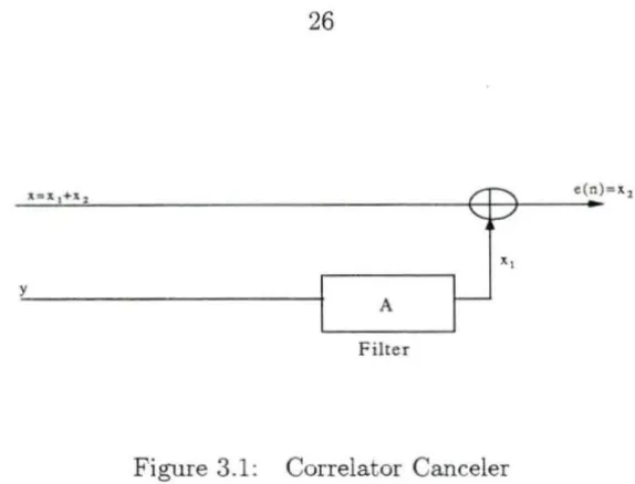
3.2 Principle of a Correlator Canceler

A correlator canceler is the best linear processor for estimating one signal from

e(n)=x₂

x, y

A

Filter

Figure 3.1: Correlator Canceler

filtering. Figure 3.1 illustrates the basic principle of a correlator canceler. If x has

a part x1which is correlated with y. Then x1 is will be canceled as much as possible

from the output so as to minimize the mean square error. The correlator canceler is

the optimal estimate of x from y. It can be viewed as an optimal signal separator

that cancels that portion of x which is correlated with y . The adaptive noise canceler

is based on the principle of a correlator.

The basic noise canceling situation is illustrated in Figure 3.2. A signal is trans-mitted over a channel to a sensor that receives the signal plus an uncorrelated noise

v(n) . T he combined signal and noise x(n)

+

canceler. A second sensor receives a signal and uncorrelated noise that is

y(n).

sensor provides the reference input to the canceler. The noise v(n) is filtered to

pro-duce an output d(n) that is a close replica of x(n). If one knew the characteristics of the channels over which the noise was transmitted to the primary and reference sensors, one could in general design a fixed filter. Noise free output from a fixed filter

x(n)=q(n)+l(n)+v(n) Primary Signal

Reference Signal

0 -N

LeakyLMS

t - - -- - - 1

Adaptive Filter

...__

__

y(n)=q(n-N)+l(n-N)+v(n-N)

Figure 3.2: The Leaky LMS

e(n)

" x(n)

characteristics of t he ideal fixed filter would have to be adjusted with a precision

dif-ficult to attain, and the slightest error could result in increased noise at the output. In the system shown in Figure 3. 2 a slight modification of the above scheme is used. The reference input is derived from the primary input. The reference is delayed by

N samples. The value of N was found by empirical methods. From t he principle of

the correlator canceler, it is lmown that for Figure 3.2

(3.1)

where

R

hence solving (3.2) we get

(3.3)

Let x be composed of the following

x(n) = q(n)

+

+

Where q(n) is the ECG signal which is observed from beat-to-beat. l (n) is the late

potential which is also observed from beat-to-beat and v(n) is the white noise. Let

y(n) consist of the following signals i.e.,

y(n) - q'(n)

+

+

(3.5)

y(n) - q(n - N)

+

+

y(n) is derived by delaying x(n) by N samples. Hence (3.2) becomes

E (

eyH)

+

+

q'

+

+

yH)

(3.6)

The assumption made is that E[vv'] = 0 after the data is shifted by N samples and

that E[qq'] and E [ll'] are non zero after a delay of N samples. Hence from (3.3) and

(3.6). we can show that

~ R R-1

where s(n) = l(n)

+

In practice we assume that the autocorrelation of the white noise is not significant after about 50 samples. The signals are strongly correlated within this lag. Any gradient descent algorithm can be used to reach this optimum Wiener solution. The Leaky LMS algorithm is discussed below.

3 .3 LMS and the Leaky LMS

The mean square error performance surface for the adaptive system is a quadratic function of the weights when the input and the desired response are statistically stationary. The task is to seek the minimum point on the performance surf ace. The LMS algorithm uses a special estimate of the gradient. The LMS algorithm is important because of its simplicity, ease of computation and because it does not require off-line gradient estimations or repetitions of data. The Leaky LMS is a variant of this algorithm. An equivalent leaky LMS can be realized by adding white

noise of mean zero and variance a to the tap-input vector of the conventional LMS

algorithm. The time varying cost function is defined as follows

J (n) =

le (n)l

llw (n)ll

where w(n) is the tap weight vector of the transversal filter , e(n) is the estimation

error and a is a constant. The error surface can be rewritten as

J ( w) = a~ - wH P - pH w

+

+

8J

-

_aw·

= -P + Rw+ aw

Hence the recursive equation to calculate the weights can be easily derived as

w

+

w

8

81

w•

Hence we can derive the update equation as follows

w

(n

+

µa)

w

(n)

+

µU(n)e•(n)

Where 0 ~ a ~ ₁ ~ µ

(3.10)

(3. 11)

(3.12)

The Wiener solution can also be derived by taking the expectations on both

sides of (3.12) and its given as follows

CHAPTER 4. DY NAMIC TIME WARPING

4.1 Introduction

Ventricular late potentials are time varying signals. Coherent averaging of these signals can be achieved if this fluctuation in time is avoided. Linear time normal-ization techniques are insufficient to deal with highly non-linear fluctuation. The dynamic programming - matching technique was studied by Sakoe and Chiba for speech recognition [28]. It is well known that speaking rate variation causes nonlin-ear fluctuation in a speech pattern time axis. Elimination of this fluctuation is called time normalization. The time-axis fluctuation is approximately modeled with a non-linear warping function with some carefully specified properties. Timing differences between two speech patterns are eliminated by warping the time axis of one to the that of the other. Then the time normalized distance is calculated as the minimized residual distance between them. This minimization process is very efficiently carried out by use of dynamic programming. This technique is used to obtain a coherent time averaging scheme with ECG signals in this thesis. An optimum algorithm for dynamic programming matching is shown in (28]. There are two kinds of dynamic

programming algorithms, the symmetric and asymmetric algorithm. In the

asym-metric form, time normalization was achieved by transforming the time axis of one

/ /

/ /

; ---Adjustment window---.-,,,

/ /

J

b1 ···;r-(··· .. ···-~-, Ck(l,J) ,,, ,,,

/ / ,,. · ~ /

/

j=i+r ,,, ,,,

/ / / / / .' : / / warping function y / : / : / / / / / : / :

b ... ,,, ... . j / C(i,j)

B

,,, ,,, j=i-r

Figure 4.1: The Warping Function

a temporarily defined common axis. A slope constraint is introduced. This is done

so that t he flexibility of the warping function is restricted. If the warping function is

4.2 Warping Principle

The signal can be expressed by appropriate feature extraction as a sequence of feature vectors.

( 4.1)

Consider the problem of eliminating the timing differences between those two

pat-terns. In order to clarify the nature of time-axis fluctuation or timing differences,

let us consider an i - j plane as shown in Figure 4.1 where

A

B

along the i- axis and j- axis respectively. Where these signal patterns are of the

same category, the timing differences between them can be depicted by a sequence of points c =

(i,j).

F = c(l ), c(2) , ... c(k), ... c(K )

(4.2)

where

c(k) = (i(k),j(k)) (4.3)

This sequence can be considered to represent a function which approximately realizes

a mapping from the time axis of pattern A onto that of B. It is called a warping

function. When there is no timing difference between these patterns, the warping

function coincides with the diagonal j = i. It deviates further from the diagonal line

d(c) = d(i ,j) =

llli -

Then the weighted swnmation of distances on the warping function

F

K

E ( F)

=

L

(4.5)

k = l

(where

w(

to allow the E(F) measure, a flexible characteristic) and is a reasonable measure

for the goodness of the warping function F . It attains its minimum value when a

warping function F is determined so as to optimally adjust the timing difference.

This minimum residual distance value can be considered to be a distance (between

patterns A and B ) still remaining after eliminating the timing differences between

them, and is naturally expected to be stable against time-axis fluctuation. Based on

these considerations, the normalized distance between two signal patterns A and B

is defined as follows:

[

~

D (A, B) = _k=_l_K _ _ _

L

k = I

(4.6)

where the denominator is employed to compensate for the effect of K (number of

points on the warping function

F).

4.2.1 Restrictions of the Warping Function

The warping function F , defined by (4.6) is a model of the time-a'Cis fluctuation

in a given pattern. Accordingly, it should approximate the properties of actual

time-axis fluctuation. In other words, function

F,

pattern

A

monotonicity, slope limi ta ti on and so on. These considerations can be realized by the following restrictions on the warping function F (or points c( k)

= (

1. Monotonic conditions

i(k - 1) $ i(k) and j(k - 1) $ j(k)

2. Continuity conditions

i(k - 1) - i(k) $ 1 and j(k - 1) - j(k) $ 1

As a result of the two restrictions the following relation holds between two con-secutive points.

(i(k), j(k) - 1)

c(k - 1) = (i(k) - l ,j (k) - 1)

(i(k) - l ,j (k))

3. Boundary conditions

I(l)

j(l)

I (K ) = I , J(K)

J

4. Adjustment window condition Figure 4.1

where r is an appropriate positive integer called window length. This condition corresponds to the fact that time-a.,"'<is fluctuation in usual cases never causes an excessive timing difference.

5. Slope constraint condition

Neither too steep nor too gentle a gradient should be allowed for warping function

F because such deviations may cause undesirable time-axis warping. A very steep

gradient, for example, causes an unrealistic correspondence between a very short

pattern

A

B

slope constraint condition, was set upon the warping function F. This is shown in

Figure 4. 2. If the point c(

k)

I

J)

m times, then the point c( k) is not allowed to step further in the same direction before

stepping at least n times in the diagonal direction. The effective intensity of the slope

constraint can be evaluated by the following measure P =

n/m.

The larger the P measure, the more rigidly the warping function slope is

re-stricted. When P = 0, there are no restrictions in the warping function. When

P = oo (that ism= 0), the warping function is restricted to diagonal j - i. Nothing

more occurs than a conventional pattern matching; no time normalization. Gener-ally speaking, if the slope constraint is too severe, then time-normalization would not

work effectively. If the slope constraint is too lax, then discrimination between signal

m times _{m times}

Minimum slope Maximum slope

C(k-1)

Symmetric Form _{Asymmetric Form}

Figure 4.2: The Different Warping Algorithms

4.2.2 Weighting coefficient

If the denominator in ( 4.6) called the normalization coefficient is independent of

the warping function F , this simplifies the equation as follows:

D (A,B) -

~mjn l~d {c(k))w{k)l

(4.7)

K

N

-

l: w(k)

This simplified problem can be effectively solved by use of the dynamic programming technique. There are two typical weighting coefficient definitions which enable this simplification. The theory is described as follows:

1. Symmetric form:

w(k) = (i(k) - i(k - 1)

+

then N = I +J where I and J are the length of the patterns A and B respectively.

2. Asymmetric form:

w(k) = (i(k) - i(k - 1)

then N = I. The basic concepts of the symmetric and asymmetric forms were

originally defined by Sakoe and Chiba [28].

4.3 Practical DP matching Algorithm

4.3.1 DP equation

A simplified definition of time-normalized distance D (A, B) as given by (4.7) is

one of the typical problems to which the well known DP-principle can be applied. The basic algorithm for calculating ( 4. 7) is written as follows.

Initial condition

DP equation:

91(c(l)) = d(c(l))w(l)

Time normalized distance:

1

D(A, B)

Ngkc(K)

It is implicitly assumed that c(O)

=

=

form, and w(l) = 1 in the asymmetric form. The restriction on the warping function

is realized by incorporating the weighting coefficient w( k). The algorithm for the

symmetric form in which no slope constraint is employed is described in (4.9). The initial condition is given by

D.P. equation:

g(l , 1) = d(l , 1)

g(i , j - 1)

+

g(i, j ) =min g(i- l,j-l)+d(i, j )

g(i - 1)

+

j)

The restriction condition (adjustment window)

Time normalized distance:

1

D(A, B )

-

Ng(I,

J )

where N I + J

The algorithm, especially the DP equation, should be modified when the asymmet-ric form is adopted or some slope constraint is employed. Chiba [28] summarizes

algorithms for symmetric and asymmetric forms. A flow chart is given in Figure 4.3

which describes the algorithm.

4.3.2 Calculation

DP equat ion of g(i,

j)

respect to coordinates I and J , starting from initial condition at (1, 1) up to

(I ,

The domain in which the DP equation must be calculated is specified by

1

<

1

<

start

i=l j=l

lntial Condition

1, 1)=d(l,1)

i=i+l

DP Equation

g(ij)=min(.)

j=j+l

T.N

distance

D(A,B)=g(l,J)/N

stop

Figure 4.3: Flow Chart for DTW

l=J-f

CHAPTER 5. TIME - SEQUENCED ADAPTIVE FILTER

5.1 Introduction

Late potentials are time varying signals and the location of this time varying

signal can be identified as l50msec after the occurrence of the R wave in the ECG

waveform. Therefore a time varying filter will be able to catch the variations of the late potentials on a beat-to-beat basis. A new form of adaptive filter was proposed by Ferrara and Widrow [29] which will be used for the estimation of a class of non-stationary signals. This new filter, called the time sequenced adaptive filter is an extension of the LMS adaptive filter. Both the LMS and the TSAF are digital filters composed of a tapped delay line, whose impulse response is controlled by an adaptive system. For stationary stochastic inputs, the mean- square error, which is the expected value of the squared distance between the filter output and externally supplied desired response, is a quadratic function of the weights. This is a paraboloid with a single fixed minimum point which can be sought by gradient techniques like the LMS. For non-stationary inputs however, the minimum point, curvature, and orientation of the error surface could be changing over time. The TSAF uses multiple

(s+n₀)j - - - .

Time Sequenced Adaptice Filter

e. _J

Figure 5.1: Symbolic Representation

so that each set of weights is associated with a single error surface. After a number of adaptations of the weights, the minimum point of each error surface is reached

resulting in a time-varying filter. For this filter, some apriori lmowledge of the input is assumed. For pulse type signals, this could be the location of the pulses in time. For signals with periodic statistics, lmowledge of the period is sufficient. This method

was used to enhance fetal electrocardiograms against background muscle noise (30].

5.2 TSAF algorithm

An adaptive transversal filter consists of a tapped delay line connected to an adaptive linear combiner that adjusts the weights of the signals derived from the

vector Xi of the adaptive linear combiner is defined as

(5.1)

The input signal components are assumed to appear simultaneously on all input lines

at discrete times indexed by the subscript j. T he weighing coefficients or multiplying

factors wo, w1 , W2 ... Wn· are adjustable. The weight vector W is

The output Yi is equal to the inner product of Xi and W

Yi=

(xfw)

The error ei is defined as the difference between the desired response di and the

actual response Yi

In adaptive filtering applications the desired response is usually composed of some underlying signal to be estimated plus additive noise uncorrelated with both the

signal and the filter input. Assume that the sequence of pairs { {di, XJ}} : ₁ is a stochastic process which need not be stationary. The expectations are taken over the

ensemble described by this stochastic process. The correlation matrix at time j as

defined by

e/w)

/

/ /

/ / / /

/~W2

Figure 5.2: Time Varying Error Surface

The mean square error at time j is given by

The error surface is a quadratic function of the weight vector at any particular

changing over time as shown in Figure 5.2.

If,

signal vectors are jointly stationary then the statistics Ri and Pi are constant, and

only a single error surface needs to be considered. In this case the gradient search

method can be used to find the minimum. The Leaky LMS algorithm was adopted.

wj

Signals composed of recurring pulses in noise are highly non-stationary due to their time-varying statistical character. The LMS adaptive filter , which is able to track such rapidly varying non-stationarities, essentially converges to the best time-invariant filter.

5.2.1 Filter Description

T he signals to be considered are those whose statistical properties recur at

var-ious points in time called regeneration times. It is required that the autocorrelation

matrix Ri and the cross-correlation vector Pi at any particular time are elements of

some finite set and they occur in identical sequence after each regeneration time. The times between regenerations are allowed to be variable. Thus the entire sequence of

R

of regeneration starts the sequence over. There exists a sequence of error surfaces as show in Figure 5.2. The TSAF proposed uses a multiplicity of weight vectors usually

one corresponding to each error surface. Since the number of different error surfaces for a statistically recurring processes is finite, the number of weight vectors is also

is selected, based on the error surface present at that instant and is adapted towards the minimum error surface. When the minimum surface is reached the weight vector

is the Wiener weight vector (optimum weights obtained by the Wiener solution) for that error surface, yielding a minimum mean squared error filter at that 'station' at that time. Thus each weight vector becomes an expert in filtering a particular

portion of the interval between regenerations. For this procedure an external input

to the filter , called the sequence number Sj is used to determine the appropriate

weight which is used at time j. Thus when Sj = i the ith error surface is assumed

to be present, so that the ith weight vector is used to form the filter output and

then adapted towards the bottom of the error surface. In order to set the sequence

number some a priori knowledge of the filter input is required. For pulse type signals, apriori knowledge could be the location of the pulse in time. For signals with periodic statistics (sometimes referred to as cyclostationary) t he knowledge of the period is sufficient. Mathematically t he TSAF algorithm is

where

Wi(j)

each weight vector. This is done in order to keep the percent loss in the steady-state performance (due to the adaptive process referred to as misadjustment) the same for

5.2.2 Disadvantages of t he TSAF

In some applications, due to uncertainty in s; at any particular time, error is

introduced at the output. The performance in the face of uncertainty in s; was

analyzed by Ferrara [29]. If the sequence number can be chosen perfectly, then it

can be shown that the TSAF converges to the optimal (minimum point of each error surface is reached) time-varying filter when the adaptation is performed slowly enough. Although in comparison with the LMS, the computational complexity is the same, the TSAF is an expensive approach to signal processing.

The number of data points required for the TSAF filter to converge to its time-varying solution is greater than that required for a conventional LMS based system. The memory requirement to implement this filter is large due to the multi-weight vectors (memory must be allocated to store the filter weights).

5.2.3 Typical Applications

The increased performance resulting in the time-varying solutions compensates

for the disadvantages in the TSAF. One application of the time-sequenced filter was to fetal electrocardiography. The location of the fetal pulses in time must be estimated in order to synchronize the filter time-varying impulse response to the fetal cardiac

5.3 Proposed Scheme to Detect Late Potentials

The late potentials are modeled as described in Chapter 6. The late potentials

are then added to the

R

Two separate channels are required. The channels have correlated signal components but uncorrelated noise components. A leaky LMS algorithm which was found to yield a high SNR in comparison with the conventional LMS (other adavantages of the leaky LMS are discussed in (27]), was used to find the weights.

Figure 5.3 describes the proposed scheme. In both channels, the X lead data

was used. White noise from two different sources was added to both the channels.

Synthesized late potentials were added to both the channels. It is assumed that the

electrodes are placed close together, but far apart so that the muscle noise in both

the channels is uncorrelated. The sequence number used is the

R

requires knowledge and location of the Late potentials. This information is available

from a

R

R

approximately 3msec. The data was sampled at 1000 Hz and the regeneration times

were from around 500msec to 650msec in the QRS waveform. Simulations were

performed for different tap sizes and different µ for the Leaky LMS algorithm. The

Xlead

Channel

Xlead

Channel

l.akylMS Adapuve Filter

Lea.ty l MS Adaptive Filte<

Lea.ty LMS Adapuve Mle<

Lea.ty LMS

Adaptive

Filter

.-· ·-.. ~

R wave is used as lhe sequence number

rror

Figure 5.3: P roposed TSAF to Detect Late Potentials

CHAPTER 6. SIMULATION RESULTS

6.1 Data Acquisition

The data were acquired through a commercial signal averaged ECG device. The

data was sampled at lOOOHz and had a resolution of l.25µv

/ bit.

about 15 minutes worth of raw ECG from the three orthogonal leads. Data are made available from two patients. The first set of data was used as control and the other as the VT inducible case. Signal averaged data was also acquired from a database. This database consisted of 18 patients. The data contained only signal averaged

ECG's, i.e., one QRS beat for each of the XYZ lead and about 600 samples long

and the data was sampled at lOOOHz. The data are only used to create and test the signal averaged ECG i.e. calculation of QRS endpoint and actual detection of late potentials. The four pole Butterworth filter was applied to this data and the R..\/IS value was calculated and compared with results available in the database. T ypical

1000

...

1000 5000

Yl.EAO

...

-«J0.'----1 ... ,-...-~2000---3000,.,._,. ,,.,.._

__

~

2000,~-~--~--~--~----...,

'"'°

-1 0000'----,~----2000~--3000~--<000~---' ....

TnMt--->f't\9«

1000

i 500

a

~

< 0

Allignment of ORS beats

.. : .... . ... . · ...

. . ···

... : -~ . . . : .

... ~ . : ~

,_.

: .1 :

: .

:

::·

600 ₈₀₀

1200 Tlm&-->msec

Figure 6. 2: Time Averaging

6 .2 Simulation methods

6.2.1 Signal Averaging

...

50

Number of OR

The data were aligned using a QRS detection algorithm [26]. The

R

used to align the beats. Ectopic (noisy) beats were rejected. A typical time average

after the R wave detection is shown for the X lead in Figure 6.2.

are shown in Figure 6.3.

6.2.2 LMS and Leaky LMS

The data for the three leads is passed through an adaptive line enhancer. The data was first scaled (by 1000) before it was passed through the filter. Both the LMS and the leaky LMS algorithm was run on the filter. Simulations were carried out for different filter tap sizes and different step sizes. The optimum filter length was

found to be 64 taps and the value ofµ and

f3

.099 and .06 respectively. These values were obtained by trial and error. Figure 6.4

compares the signal average, LMS and leaky LMS for the X Y and Z lead. 'rhe leaky

LMS algorithm was also run on the :Y.lotorola 56K. The data was scaled before it was input to the fixed point DSP. The scaling factor was 1000 so that the data fell in the

range of

±1.

of the beat-to-beat noise level. In Figure 6.4 (X lead data) , the performance of the Leaky LMS algorithm yields lower noise levels on a beat-to-beat basis in comparison to the LMS. Similar results were observed for all the other orthogonal leads. The root mean square value was calculated and compared. The RMS values obtained by signal averaging before and after the LMS algorithms are shown in Figure 6.7. The Rl\IIS was evaluated on a beat-to-beat basis to show the feasibility of the algorithm. This is shown in Figure 6.8. The Rl\IIS value shows a clear reduction in the beat-to-beat noise level.

-·.~--=--=---=-,.--__..,,.,..-~---..,:

_...

-,..._,

...

-·-·.!-

-._....zi...-:--....

--.'---~---'

--• ..._, _ ..

,"-'ll~lt.--~

1:

i:

~·,.'----=-~=---=-,..---=--~---..,:

• ..._ .,..,_ T.._

-II

.II

1~

-.'---,.,,--~---=-,--__..,,.,..--=---=­

.__...,.._.Z"-"

•• _., I

... '---'----~---=--.,.,.,.____,,_

~=

i

L., ..

Figure 6.4:

IOO . ... •··•••·•·•·· ... ... _ ..•.. - · ·

···-500 1000 15(1) 2DCO 2500 X1CO 3500 4000 4500 5CXX1 _{r.,.. _ _ -200 Q :IQO 1 ODO l SIO 2CD> 2'°° lalO} 3!!00 «XlO 4SXI 5CXXJ

ECG X l.oad M.-~ lMS

-2000'----'soo~-,~ooo~-,~soo~-2000-'--~2500....__3000_._~""°"-'-~ ... -'-~4500-'----'sooo

Ti~->l'NOC

rm ... -~ .. c:

The X Lead: Raw X Lead, Output of LMS Based Adaptive filter and

~ECGYL.em

...

...

...

-

--- IOOO 500 1000 1500 2000 ZSOO lOOO lSOO ,...,..

__

ECO V .._ .,._ ._ky IMS

SJO ....

1-... ..

I .

...200 ....

-eoo₀~-..,...._-, ... .,.--, ... -,...,=-2SC0=~3000.,.,_..,.,lli00.,.,..._•ooo.,.,..._<SOO.,.,..._..,,..sooo ,...,..

__

~--~

1SOO 1500

- tOOO O 500 1000 1500 2000 2500 3000 l500 «>00 4500 SOCIO _,...,.___._

_

_..____.~_._

_

_

0 500 1 000 I IOI) 2CXIG 2500 3000 35QO 4000 4500 5000

.,..,,._,.,.... Tirne- -- ~

£CO Z L..m An• LNky LMS