Grey Forecast Model for Accurate Recommendation to
Cope with Data Sparsity and Correlation
Feng Xie
*†, Jiaxing Shang
*†, Zhen Chen
†‡, Geoffrey C. Fox
§ *Department of Automation, Tsinghua University, Beijing, 100084, China
†
Research Institute of Information Technology, Tsinghua University, Beijing, 100084, China
‡
Tsinghua National Lab for Information Science and Technology, Beijing, 100084, China
§School of Informatics and Computing, Indiana University, Indiana, 47408, USA
{xief10, shangjx06}@mails.tsinghua.edu.cn, [email protected], [email protected]
ABSTRACT
Recommender systems attracts more and more attention recently, as they can suggest appropriate candidates to users based on intelligent prediction. As one of the most popular recommender system techniques, Collaborative Filtering achieves efficiency from the similarity measurement of users and items. However, existing similarity measurement methods cannot guarantee accuracy due to data correlation sparsity. Consequently, the prediction suffers from low accuracy. To overcome these problems, this paper introduces the Grey Forecast model for recommender systems. Firstly, the Cosine Distance method is used to compute the similarities between items. Then we rank the items according to their similarities and select the k most similar items’ ratings that active users have rated as input to construct a Grey Forecast model and yield predictions. The novelty of the paper is two-fold: less data is required in constructing the model, and the model will become more effective when there are strong correlations. Our approach was evaluated on two public data sets: MovieLens and EachMovie. The experimental results show that the proposed algorithm can significantly overcome the limitation of the data sparsity and benefit from the data correlation. Especially, with the MovieLens data set, the accuracy has been improved by over 20% in terms of Mean Absolute Error (MAE) and Root Mean Square Error (RMSE), even with very small k.
Categories and Subject Descriptors
H.3.3 [Information Systems]: Information Search and Retrieval – Information Filtering
General Terms
Algorithms, Measurement, Performance, Experimentation.
Keywords
Recommender Systems, Collaborative Filtering, Grey Forecast Model, Correlation, Sparsity.
1.
INTRODUCTION
Recommender systems help users cope with information overload in a wide range of Web services and have been broadly adopted in
various applications, such as E-commerce (e.g. Amazon1), online video sharing (e.g., YouTube2) and online news aggregators (e.g. Digg3). It presents the most attractive and relevant items to the user based on individual user’s characteristics. As one of the most promising recommender techniques [1], Collaborative Filtering (CF) predicts the potential interests of an active user by considering the opinions of users with similar taste. Compared to other recommender techniques (e.g. content based method [2]), collaborative filtering technologies have the capability to recommend to users surprising items which aren’t similar to what they have seenbefore, and could work well in domains where items’ attribute content are difficult to parse. Generally, the representative Collaborative Filtering technique, memory based CF, has been widely used in many commercial systems due to its simple algorithms but reasonably accurate recommendation. Thesecapture the user’s ratings on different items explicitly by asking the user or implicitly by observing his/her interaction with the systems to store them into a table known as the rating matrix. Then, memory based CF methods use similarity measurement methods to filter users (or items) that are similar to the active user and calculate the prediction from the ratings of these neighbors. Memory based methods can be further classified as user based method [3] or item based method [4] depending on whether the process of defining neighbors by finding similar users or similar items.
Despite its widespread adoption, memory based CF still suffers from several major problems including the data sparsity problem [1][8], data correlation problem [5], and cold start problem [6][7]. The cold start problem can be regarded as data sparsity problem. Hence, in this paper, we focus on the former two issues. In most recommender systems, each user rates only a small subset of the available items, thus, most of the entries in the rating matrix are empty. In these cases, it is a great challenge to find similar users or items. Consequently, the similarity between two users or items cannot be calculated and the prediction accuracy will be very low. Furthermore, the active users always tend to consume similar commodities and the ratings for these items will be close, which produces strong correlations among the ratings. However, the existing similarity measurement methods, such as Cosine Distance and Pearson Correlation, cannot well cope with these issues. Therefore, we can’t directly use the similarities for rating prediction. To overcome these problems, some researchers have developed algorithms that use models to generate predictions [9][10][11]. However, many models are extremely complex, and have multiple parameters to estimate and are always too sensitive
1
www.amazon.com/ 2
www.youtube.com 3
www.digg.com
Permission to make digital or hard copies of all or part of this work for personal or classroom use is granted without fee provided that copies are not made or distributed for profit or commercial advantage and that copies bear this notice and the full citation on the first page. To copy otherwise, or republish, to post on servers or to redistribute to lists, requires prior specific permission and/or a fee.
to data changes. In practice, many of these theoretical models are not effective.
In this paper, we present novel approaches that aim at overcoming data sparsity limitations and benefit from the data correlations among the ratings and do not eliminate them. More specifically, the proposed algorithm calculates the similarities between items with the simplest method, Cosine Distance measurement method. Note that, we don’t use the exact value of the similarities, and just rank the items according to these similarities. Then the Grey Forecast model is used for the rating prediction. This has been successfully adopted in many fields, such as finance [12], integrated circuit industry [13], the market for air travel [14], and underground pressure for working surface [15]. We compare the performance of the proposed algorithm with traditional user based and item based methods in terms of two evaluation metrics MAE and RMSE on two datasets MovieLens and EachMovie. Our results provide empirical evidences that Grey Forecast model indeed can well cope with data sparsity and correlation problems.
The remainder of this paper is organized as follows. Section 2 provides a detailed description of traditional user based CF method, item based CF method, the definition of the problem, and our contributions. Section 3 presents our proposed Grey Forecast model based algorithm in detail. Section 4 describes the experimental study, including experimental datasets, evaluation metrics, methodology, analysis of results, followed by a final section on conclusions and future work.
2.
RELATED WORK
Collaborative Filtering (CF) is one of the most successful recommender techniques [16], and it includes memory based CF techniques such as similarity based or neighborhood based CF algorithm; model based CF techniques such as clustering CF algorithms; and hybrid CF techniques such as personality diagnosis. As a representative memory based CF technique, similarity based methods represent one of the most successful approaches to recommendation. Notably they have been deployed into commercial systems and been extensively studied [1][17]. This class of algorithm can be further divided into user based and item based methods. The former is based on the basic assumption that people who have similar past preferences tend to agree in their future tastes. Hence, for the target user, the potential interest on an object is predicted according to the ratings from users who are similar to the target user. Different from user based method, item based method recommends a user the items that are similar to what the active user has consumed before. In a typical memory based CF scenario, there is a set of n users U= {u1, u2,..., un} and
a set of m items I= {i1, i2,..., im }, and the
n
×
m
user-item rating [image:2.612.342.530.66.233.2]matrix. The ratings can either be explicit indications, such as an integer number varies from 1 to 5, or implicit indications, such as purchases or click-throughs [18]. For example, the implicit user behaviors (Table 1(a)) can be converted to a user-item rating matrix (Table 1(b)), where the (k,l) in k-th row and l-th column of the matrix stands for the k-th user’s rating for the l-th item. Would the k-th user have not rated the l-th item yet, the null value is assigned to (k,l). Thus, the recommendation problem is reduced to predicting the unrated entries (Lily is the active user that we want to make recommendations for in Table 1(b)). Generally, the process of this type of CF methods consists of two steps: similarity measurement and rating prediction.
Table 1. An example of a user-item rating matrix
(a)
User Purchase Not purchase
Alic e
Milk, Bread, Cake Beer
Lily Milk, Bread Cake, Beer
Lucy Milk, Cake Bread, Beer
Bob Bread, Beer Milk, Cake
(b)
Bread Beer Cake Milk
Alice 1 1 1
Lily 1 ? 1
Lucy 1 1
Bob 1 1
2.1
Similarity Measure
The critical step in memory based CF algorithms is the similarity computation between users or items. In user based CF methods (UCF), the similarity s(ux,uy)between users uxand uy is found by
comparing the items that both have rated. For item based CF methods (ICF), the similarity s(ix,iy) between items ix and iy,
isdetermined by the users who have rated both of the two items. There are various methods to compute similarity between two users or items. The two most popular methods are Cosine Distance [2][19] and Pearson Correlation [2][19]. To define them, let I be the set of all items rated by both users uxand uy, and let U
be the set of all users who have rated both items ixand iy. Then,
the co-rated entries related to object (ux, uy, ix,or iy) form a d
-dimensional vector, where d is equal to the size of set I or U. For example, in Table 1, the co-rated items of Alice and Lucy are
Cake and Milk, therefore, d is equal to two in such case.
2.1.1
Cosine Distance
For Cosine Distance approach, the cosine of the angle between the vectors represents the similarity between them (see Figure 1). It can be formulated as:
2 1
2 1
cos ) 2 ,
1 (
object object
object object
d d
d d object
object
s
⋅ =
=
θ
(1)Where “
⋅
” denotes the dot-product of two vectors, and “ ” isthe vector modulus.
d
object (object1 and object2 can be the pair ofux and uy, or ix andiy) is a d-dimensional vector constructed by
the interactions of the objects. Therefore, the bigger the cosine of the angle (θ), the more similar the two objects will be.
Figure 1. The representation of cosine distance.
2.1.2
Pearson Correlation
We should note that, in the computation of similarity, it is necessary to eliminate the correlation among the ratings, which is also known as rating correlation, such as the average rating of the
θ
1object
d
2
[image:2.612.396.491.566.633.2]user, otherwise the similarity is less meaningful. The Pearson Correlation is one method of this type which can improve the accuracy of similarity computation to a certain extent. For UCF, the Pearson Correlation between two users is:
(
)
(
)
(
)
∑
(
)
∑
∑
∈ ∈ ∈−
−
−
−
=
Ii u i u I
i u i u I
i u i u u i u y x y y x x y y x x
r
r
r
r
r
r
r
r
u
u
s
2 , 2 , , ,)
,
(
(2)Where u i
x
r
, , ruy,iare the ratings of users ux, uy on item i and
x
u
r
,y
u
r
are the average ratings of users ux, uy, respectively.Similarly, for ICF, the Pearson Correlation between two items can be formulated as:
(
)
(
)
(
)
∑
(
)
∑
∈∑
∈ ∈−
−
−
−
=
Uu ui i U
u ui i U
u uix i ui i y x y y x x y y x
r
r
r
r
r
r
r
r
i
i
s
2 , 2 , , ,)
,
(
(3)Where
x
i u
r
, ,r
u,iyare the ratings of user u on items ix, iy and
x
i r ,
y
i
r are the average ratings of all users on items ix, iy,
respectively.
2.2
Rating Prediction
The phase of rating prediction aims to predict the value that the active user will give to the target item. The KNN-based method is usually utilized to generate predictions by weighting sum of the ratings that similar users give to the target item or the ratings of the active user on similar items depending on whether it uses UCF or ICF.
2.2.1
User based CF (UCF)
The UCF algorithm is based on the basic assumption that people who share the similar past tastes will be interested in same items. The algorithm uses the following steps: the first step is to compute the similarities between users with the similarity measurement methods introduced in section 2.1; and then produce the prediction for the active user by taking the weighted average of all the ratings of the user on a certain item [20] according to the following formula; finally, the item with high predicted ratings will be recommended to the user.
∑
∑
∈ ∈−
+
=
) ( ) ( , ,)
,
(
)
)(
,
(
u U v u Uv vi u
u i u
u
v
s
r
r
u
v
s
r
p
(4)Where
r
uis the average rating of user u; s(v, u) is the similarity between user v and user u calculated using similarity measure given in section 2.1; and U(u) denotes the set of similar users of user u.p
u,i is the prediction of user u on item i.2.2.2
Item based CF (ICF)
The ICF algorithm recommends to users items similar to those already consumed. Similarly, after calculating the similarities between items, the unknown rating of user u on item i can be represented as an aggregate rating of user u on similar items:
∑
∑
∈ ∈=
) ( ) ( , ,)
,
(
)
,
(
i I j i Ij uj
i u
i
j
s
r
i
j
s
p
(5)Where s(j, i) is the similarity between items j and i calculated using similarity measurement methods given in section 2.1; and
I(i) denotes the set of similar items of item i. pu,i denotes the
prediction of user u on item i.
2.3
Problem Analysis
After using the co-rated entries as a vector to represent the object, the Cosine Distance measures the similarity between two users or items by computing the cosine of the angle. The bigger the value is, the more similar the two users or items will be. Pearson Correlation takes the rating correlation into consideration to eliminate the influence of average rating. Obviously, this class of similarity measure is a variation of Cosine Distance. Taking UCF as an example, we pick the items that both users have rated before, and then use the ratings of each user on these items to construct a
d-dimensional vector such as
(
)
d i u i u i
u
r
r
r
,1,
,2,
⋅
⋅⋅
,
, , where d is the number of co-rated items. If we subtract each element by theaverage rating of user u, the vector will be changed
to
(
r
uir
ur
uir
ur
uir
u)
d
−
⋅⋅
⋅
−
−
, ,,1
,
2,
,
. In this case, the PearsonCorrelation is equivalent to Cosine Distance. With Pearson Correlation, the accuracy of similarity computation can be improved to a certain extent. However, it still suffers from many disadvantages.
Data Sparsity. It’s difficult to find co-rated entries when
the data is sparse. For instance, Bob and Lucy haven’t consumed the same items before (Table 1). Thus, the similarity between them cannot be computed with existing methods in section 2.1. Furthermore, the similarities between users or items may not be obtained in the same dimensionality. For example, Alice and Lucy both rated milk and cake (Table 1), the similarity between them is computed in 2-dimensional spaces; while Bob and Lily just have one co-rated entry, bread (Table 1), the similarity between them is computed in 1-dimensional space. The results are biased.
Data Correlation. In this paper, data correlation
corresponds to the common features hidden in the data coming from the similar attributes among users or items. The correlations among the ratings results in the non-orthogonal vector space since the elements in different dimensions are not independent. Although the Pearson Correlation has eliminated the influence of average rating, such rating correlations still exist. For instance, people who like Tom Cruise tend to give similar rating to movies “Mission: Impossible III” and “Mission: impossible 4”; people with same age will have similar taste, so the ratings on the same item will be close. Therefore, the similarities computed with these similarity measurement methods are not accurate.
2.4
Contributions
The process for Grey Forecast to make prediction can be described as: The Cosine Distance method is used to measure the similarity between two items. Then, a m×msimilarities matrix will be generated, where m is the number of items. Although the similarity computation is not accurate, as has been discussed in section 2.3, the value can represent the degree of similarity. Thus, in our algorithm, we don’t use the exact value of similarity but rather just rank the items according to them. Then, to generate the prediction of the active user u on item i, the k most similar items that have rated by the active user to item i are chosen. Finally, we use these items as input to construct a Grey Forecast model and predict the rating of the active user u on item i. Note that, if user u
didn’t rate k items, the fixed value 3 will be used to complete k
ratings.
With this method, there are three main contributions in this paper:
Overcome Data Sparsity. Although it is a great challenge
to find similar users or items when data is sparse, only a few neighbors are needed to construct the Grey Forecast model for our algorithm and the experimental results show that the prediction accuracy is still high even when k=5. Therefore, the proposed algorithm can efficiently overcome e the data sparsity problem.
Benefit From Data Correlation. The stronger the data
correlations are, the more accurate the Grey Forecast model will be. In other words, the proposed algorithm can efficiently benefit from the data correlations rather than eliminate them.
Obtain Accurate Prediction. We test our algorithm on two
public data sets, MovieLens 4 and EachMovie5. The experimental results compared with UCF and ICF (with Cosine Distance for similarity computation) show that our algorithm gets better performance in prediction accuracy. Especially, with the MovieLens data set, the accuracy has been improved by over 20% in terms of MAE. Moreover, the value of k can be very small without losing in accuracy.
3.
PROPOSED ALGORITHM
Memory based CF algorithms weight ratings of similar users on target item or ratings of active user on similar items to generate prediction. Consequently, the accuracy of prediction depends mainly on the similarity computation. However, when the data is sparse with strong correlations, existing similarity measurement methods cannot obtain accurate similarities between users or items. In other words, the similarities are not very meaningful. Hence, we cannot use the similarities to produce a reliableprediction directly. In this paper, the Grey Forecast model is used for rating prediction. There are two steps: rating preprocessing and rating prediction.
3.1
Rating Preprocessing
Since the similarities between items computed by existing similarity measurement methods have value, we use them to preprocess the ratings. Firstly, for simplicity, the Cosine Distance method is utilized to compute the similarity between two items. Then a
m
×
m
similarities matrix will be generated, where m is4
http://www.grouplens.org/ 5
http://www.kumpf.org/eachtoeach/eachmovie.html
the number of items. If we want to predict the unrated entry of user u on item i in the rating matrix, the k most similar items to item i that have rated by user u are chosen. Note that, when user u
didn’t rate k items, the fixed value 3 with lowest similarity will be used to complete k ratings in our algorithm. Finally, the k ratings are sorted according to their similarity to item i to produce a rating sequence, where the rating with the highest similarity will stand first. In the next step, the proposed algorithm will take the rating sequence as input to construct the Grey Forecast model and forecast the rating that user u will give to item i. For instance, a fragment of a rating matrix with ratings vary from 1 to 5 is shown in Table 2. We want to predict the rating of user u3 on item i1. According to the Cosine Distance, the similarities between item i1 with other items are: 0.989, 0.789, 0.991, 0, 0.999, 0, 0.942, 0.857, and 0.999, respectively. If we set k=3, items i3, i4, and i9 will be selected, and the rating sequence is (4, 3, 5) according to their similarities with item i1, since they have rated by user u3 and have
higher similarities with item i1. Furthermore, if we set k=7, all
items rated by user u3 will be chosen, and the rating sequence is
(3, 3, 5, 4, 4, 3, 5). In such case, the number of items rated by user
u3 is less than 7, therefore, the fixed value 3 will be used to
[image:4.612.318.533.326.407.2]complete seven ratings but with lowest similarity, such as the first two numbers 3 in the rating sequence. Note that, when two or more ratings with the same similarity but the value are not equal, the order is random.
Table 2. A fragment of rating matrix
i1 i2 i3 i4 i5 i6 i7 i8 i9 i10
u1 4 4 5 5 4 4 5
u2 3 4 2 4 3 4
u3 ? 4 5 5 4 3
u4 1 3 2 3 4
The rating sequence has several special attributes:
The correlations between them are strong, since they are the
k most similar items to the target item. The similarities between them will be absolutely high. Hence, these ratings are regular not random.
This sequence can be regarded as rating sequence sorted by time. The item’s rating with highest similarity can be regarded as the latest rating of active user, which will have the biggest contribution to the rating prediction of active user on the target item. This is the reason why we sort the ratings according their similarities to the target item from low to high.
In these cases, the effective way for rating prediction is to find out the law hidden in the rating sequence and benefit from it.
3.2
Rating Prediction
of requiring less data so it overcomes data sparsity problem. The rating sequence generated in the phase of rating preprocessing is all that is needed as input for model constructing and future forecasting. These are the reason why we choose the Grey Forecast model for rating prediction, and the GM(1,1) method is adopted in this paper. GM(1,1) indicates one variable and one order Grey Forecast model. The general procedure for a Grey Forecast model is derived as follows [23]:
Step 1: Assume the original rating sequence to be
r
u(0){
(0)(
)
}
,
1
,
2
,
,
.
) 0 (
k
t
t
r
r
u=
=
⋅
⋅⋅
(6)Where r(0)(t) corresponds to the original rating of user u on the
(k-t)-th most similar item or the t-th value of rating sequence. k is the number of neighborhoods or the length of rating sequence and must be equal to or larger than 4.
Step 2: A new sequence (1)
u
r is produced by the Accumulated Generating Operation (AGO).
.
,
,
2
,
1
)},
(
{
(1)) 1 (
k
t
t
r
r
u=
=
⋅
⋅⋅
(7)Where
(
)
(
)
,
1
,
2
,
,
.
1 ) 0 ( ) 1 (
k
t
j
r
t
r
t j⋅⋅
⋅
=
=
∑
=Step 3: Build a first-order differential equation.
b
az
dt
dr
(1)/
+
=
(8)Where
z
(1)(
t
)
=
α
r
(1)(
t
)
+
(
1
−
α
)
r
(1)(
t
+
1
),
t
=
1
,
2
,
⋅
⋅⋅
,
k
−
1
.α(0<
α
<1) denotes a horizontal developing coefficient. The selecting criterion of αis to yield the smallest prediction error rate. In our experiments, we setα
=0.2, since the ratings of items with higher similarities to the specific item will contribute more to the final rating prediction.Step 4: From Step 3, we get the forecasting model GM(1,1):
a
b
e
a
b
r
t
r
ˆ
(1)(
+
1
)
=
(
(0)(
1
)
−
/
)
−at+
/
(9)
Where
a
is the development coefficient, andb
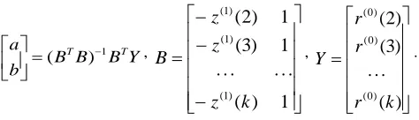
is grey action, andY B B B b
a T 1 T
) ( − = ,
−
⋅
⋅
⋅
⋅
⋅
⋅
−
−
=
1
)
(
1
)
3
(
1
)
2
(
) 1 ( ) 1 ( ) 1 (k
z
z
z
B
,
⋅⋅
⋅
=
)
(
)
3
(
)
2
(
) 0 ( ) 0 ( ) 0 (k
r
r
r
Y
.Step 5: Inverse Accumulated Generation Operation (IAGO).
Because the Grey Forecast model is formulated using the data of
AGO rather than original data, we should use IAGO to transfer the data of AGO to actual rating prediction:
)
1
(
)
/
)
1
(
(
)
(
ˆ
)
1
(
ˆ
)
1
(
ˆ
) 0 ( ) 1 ( ) 1 ( ) 0 ( a ate
e
a
b
r
t
r
t
r
t
r
−
−
=
−
+
=
+
− (10)
When we set
t
=
k
, the rating predictioni u
p, of user u on item i
can be represented by
ˆ
(0)(
+
1
)
k
r
.Obviously, during the estimate of parameters
a
andb
in Step 4, a matrix inverse operation is needed. Hence, we cannot always forecast the ratings using Grey Forecast model. In these cases, the average of k ratings is used as the rating prediction of the active user on the target item.4.
EXPERIMENTAL RESULTS
In this section, we present the results of the experimental evaluation of our novel algorithm. We describe the data sets used; the experimental methodology as well as the performance improvement compared to the traditional memory based collaborative filtering methods introduced in section 2.
4.1
Data Sets
[image:5.612.55.292.600.668.2]We deployed our proposed algorithm, as well as UCF and ICF methods on two standard datasets: MovieLens [24] and EachMovie [25]. Both of these are publicly available movie rating datasets. MovieLens rating sets were collected by GroupLens research from MovieLens web site (http://movielens.umn.edu). There are three different sizes of available data sets. In this paper, the MovieLens 1M was used, which consists of 1 million ratings (in 1-to-5 star scale) from 6,040 users on 3,952 movies. We also implemented the experiments on the other dataset, EachMovie, which was collected by DEC Systems Research Center. It consists of 2,811,983 numeric ratings of 74,424 users on 1,648 different movies (films and videos). Since the ratings are mapped linearly to the interval [0, 1], for conveniently, we multiplied the ratings by 5, and deleted the records that ratings were zero. Finally, 2,464,792 ratings were obtained, which were in 1-to-5 rating scale. Table 3 summarizes the statistical properties of both datasets.
Table 3. Statistical properties of MovieLens and EachMovie
MovieLens EachMovie
Users 6,040 74,424
Items 3,952 1,648
Ratings 1,000,000 2,464,792
Ratings Per User 165 33
Ratings Per Item 253 1495
Sparsity 95.81% 97.99%
4.2
Metrics and Methodology
predicted ratings and the user’s real ratings. MAE [26] and RMSE [27] are defined as:
T
p
r
MAE
=
∑
(u,i)∈T u,i−
u,i (11)(
)
T
p
r
RMSE
∑
ui∈T ui ui−
=
( ,)2 , ,
(12)
where T is the set of all pairs (u, i) in the test set. To evaluate the performance of our proposed algorithm we consider three comparison methods:
Grey Forecast model: The novel rating prediction model
adopted in this paper. Using Cosine Distance as the items’ similarity measurement and setting
α
=0.2. User based CF: This is well-known user based
collaborative filtering method. The Cosine Distance measurement method computes the similarity between two users.
Item based CF: This is also a memory based approach,
which calculates the similarity between two items with Cosine Distance.
4.3
Experimental Results
[image:6.612.97.252.81.156.2]Figure 2 and Figure 3 show the MAE and RMSE values of all comparison partners on the MovieLens data set.
Figure 2. The MAE value comparison of three methods on MovieLens dataset.
Figure 3. The RMSE value comparison of three methods on MovieLens dataset.
The Cosine Distance method is used for the similarity computation between users or items. Then we find k nearest
neighborhoods for them, and k is adopted as 5, 10, 15, 30, 40, and 60, respectively. For Grey Forecast model, we set the horizontal developing coefficient
α
=0.2, since the ratings of items with higher similarities to the specific item will contribute more to the final prediction. Meanwhile, if certain user didn’t rate k items, the fixed value 3 will be used with lowest similarity so that the rating sequence will always have k numbers. The results illustrated in these two figures report that Grey Forecast model based method has the lowest prediction error. Moreover, as the k increases, UCF and Grey Forecast model based method can achieve better performance, while the prediction accuracy of ICF method decreases smoothly. Because the ratings per item are more than the ratings per user (Table 3), it is easy for UCF method to find users who have rated the specific item in k nearest neighborhoods. On the contrary, for ICF method, it is difficult to find items which are rated by the active user in the k nearest neighborhoods. Therefore, UCF method presents higher accuracy than ICF method. [image:6.612.341.515.289.429.2]Similarly, Figure 4 and Figure 5 illustrate the MAE and RMSE values of all comparison methods on the EachMovie data set. The experiment design and the parameters selection are the same.
Figure 4. The MAE value comparison of three methods on EachMovie dataset.
Figure 5. The RMSE value comparison of three methods on EachMovie dataset.
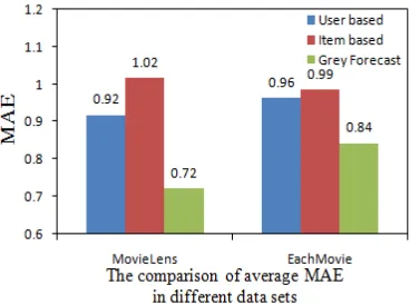
[image:6.612.76.250.365.491.2] [image:6.612.345.519.470.614.2] [image:6.612.76.259.531.660.2]better observation of the slight difference of performance among these three methods, we average the prediction error of different k
values. Consequently, the MAE and RMSE values comparison of three methods on two datasets are illustrated in Figure 6 and Figure 7, respectively.
[image:7.612.75.263.250.387.2]Obviously, for MovieLens data set, the Grey Forecast model based method reduces the prediction error in terms of MAE by 27.8% and 41.7% compared to the UCF method and ICF method, respectively. It also reduces the prediction error of RMSE by 26.6% and 35.1% compared to the UCF method and ICF method, respectively. Similarly, for EachMovie data set, the Grey Forecast model based method reduces the prediction error of MAE by 14.3% and 17.9% compared to the UCF method and ICF method, respectively. It also reduces the prediction error of RMSE by 15.0% and 15.9% compared to the UCF method and ICF method, respectively.
Figure 6. The average MAE value comparison of three methods.
Figure 7. The average RMSE value comparison of three methods.
All the results are summarized in Table 4. Moreover, since the EachMovie data set is sparser than the MovieLens data set, the prediction accuracy in the former data set outperforms that in the latter data set.
Table 4. The prediction error ratio for all methods (in %)
Data set Metrics UCF ICF
MovieLens MAE 27.8 41.7
RMSE 26.6 35.1
EachMovie MAE 14.3 17.9
RMSE 15.0 15.9
As described above, the Grey Forecast model based method yields more accurate prediction than traditional memory based CF. In our experiments, we also find that Grey Forecast model based method can achieve better performance even when the k value is very small. For the Grey Forecast model based method, we set k
equal to 5, while we set k equal to 100 for the other two methods, UCF and ICF. The MAE and RMSE values are compared, and Table 5 summarizes the comparison results. GF stands for Grey Forecast model based method.
The results in Table 5 show that the Grey Forecast model based method can generate high accuracy prediction even when the selected neighborhoods are quite small. Although the number of nearest neighborhoods reaches up to 100, the UCF and ICF methods still suffer from low accuracy.
Table 5. The MAE and RMSE value comparison of three methods with different k value
Data Set Metric UCF(100) ICF(100) GF (5)
MovieLens MAE 0.85 1.04 0.74
RMSE 1.14 1.30 0.97
EachMovie MAE 0.94 0.97 0.86
RMSE 1.20 1.23 1.11
[image:7.612.347.532.347.406.2]The ratio of prediction error between the Grey Forecast model based method and the UCF method and ICF method are given in Table 6.
Table 6. The prediction error ratio for all methods with different k value (in %)
Data set Metrics UCF ICF
MovieLens MAE 14.9 40.5
RMSE 17.5 34.0
EachMovie MAE 9.3 12.8
RMSE 8.1 10.8
Obviously, the Grey Forecast model based method perform much better on the MovieLens data set than on the EachMovie data set. The reason lies on the fact that the former is sparser than the latter. However, the Grey Forecast model based method generates more accurate prediction than the UCF and ICF methods on both datasets.
5.
CONCLUSION AND FUTURE WORK
Since the existing similarity measurement methods, such as Cosine Distance and Pearson Correlation, cannot compute the similarities between users or items accurately when the data is sparse and there exists strong data correlations, user based CF and item based CF methods couldn’t perform well in prediction accuracy. In this paper, we used the Grey Forecast model for rating prediction in recommender systems and conducted extensive experiments on two movie datasets, MovieLens and EachMovie. The experimental results demonstrated that Grey Forecast model based method can overcome data sparsity and benefit from data correlations, which outperforms traditional memory based CF methods, for both user based and item based approaches. Especially, even when only 5 nearest neighborhoods are adopted, the Grey Forecast model based method still reduces the prediction error by over 14% and 40% on the MovieLens and 9% and 12% on the EachMovie in terms of MAE compared to user based and item based methods with 100 nearest neighborhoods, respectively.
[image:7.612.76.263.426.573.2]accuracy recommendation. It opens a new era that we can use advanced technologies of other fields to construct novel recommender algorithms, which can well cope with problems in recommender systems, such as data sparsity, data relevance, and cold start. As an effective rating prediction method, the Grey Forecast model still has room for improvement. In our future work, when the user didn’t rate enough k items, we will use the average of the user’s ratings on all items instead of the fixed value 3 to complete k numbers. Moreover, we will also try to compare the performance with different similarity measurement methods for Grey Forecast model based method.
6.
ACKNOWLEDGMENTS
Many thanks to the help of Prof. Jun Li and Prof. Junwei Cao.
7.
REFERENCES
[1] Sarwar, B., Karypis, G., Konstan, J., and Riedl, J. 2000. Analysis of recommendation algorithms for e-commerce.
Proc. EC’00, 158-167.
[2] Adomavicius, G., and Tuzhilin, A. 2005. Toward the next generation of recommender systems: a survey of the state-of-the-art and possible extensions. IEEE Trans. on Knowledge and Data Engineering 17, 6 (June 2005), 734-749. [3] Resnick, P., Iacovou, N., Suchak, M., Bergstrom, P., and
Riedl, J. 1994. Grouplens: an open architecture for
collaborative filtering of netnews. Proc. CSCW’94, 175-186. [4] Sarwar, B., Karypis, G., Konstan, J., and Riedl, J. 2001.
Item-based collaborative filtering recommendation algorithms. Proc. WWW’01, 285-295.
[5] Cacheda, F., Carneiro, V., Fernández, D., and Formoso, V. 2011. Comparison of collaborative filtering algorithms: limitations of current techniques and proposals for scalable, high-performance recommender systems. ACM Trans. on Web 5, 1 (Feb. 2011), 2:1-2:33.
[6] Hu, R., and Pu, P. 2011. Enhancing collaborative filtering systems with personality information. Proc. RecSys’11, 197-204.
[7] Liu, N.N., Meng, X.R., Liu, C., and Yang, Q. 2011. Wisdom of the better few: cold start recommendation via
representative based rating elicitation. Proc. RecSys’11, 37-44.
[8] Ma, H., Zhou, T.C., Lyu, M.R., and King, I. 2011. Improving recommender systems by incorporating social contextual information. ACM Trans. On Information Systems 29, 2 (April 2011), 9:1-9:23.
[9] Lemire, D., and Maclachlan, A. 2005. Slope one predictors for online rating-based collaborative filtering. Proc. SDM’05, 471-475.
[10]Marlin, B.M., and Zemel, R.S. 2009. Collaborative prediction and ranking with non-random missing data. Proc. RecSys’09, 5-12.
[11]Paterek, A. 2007. Improving regularized singular value decomposition for collaborative filtering. Proc. KDDCup’07, 39-42.
[12]Hsu, L.C., and Wang, C.H. 2002. Grey forecasting the financial ratios. The Journal of Grey System 14, 4 (2002), 399-408. (In Chinese)
[13]Hsu, L.C. 2003. Applying the grey prediction model to the global integrated circuit industry. Technological Forecasting and Social Change 70, 6 (July 2003), 563-574.
[14]Hsu, C.I., and Wen, Y.H. 1998. Improved grey prediction models for the trans-pacific air passenger market.
Transportation Planning and Technology 22, 2 (March 1998), 87-107.
[15]Ma, D., Zhang, Q., Peng, Y., and Liu, S.J. 2011. A particle swarm optimization based grey forecast model of
underground pressure for working surface, Electronic Journal of Geotechnical Engineering 16 H (2011), 811-830. [16]Konstan, J., Miller, B.N., Maltz, D., Herlocker, J.L., Gordon,
L.R., and Riedl, J. 1997. GroupLens: applying collaborative filtering to usenet news. Communication of the ACM 40, 3
(March 1997), 77-87.
[17]Linden, G., Smith, B., and York, J. 2003. Amazon.com recommendations: item-to-item collaborative filtering. IEEE Internet Computing 7, 1 (Jan. /Feb. 2003), 76-80.
[18]Miller, B.N., Konstan, J.A., and Riedl, J. 2004. PocketLens: toward a personal recommender system. ACM Transactions on Information Systems 22, 3 (July 2004), 437-476.
[19]Herlocker, J.L., Konstan, J.A., Terveen, L.G., and Riedl, J.T. 2004. Evaluating collaborative filtering recommender systems, ACM Transactions on Information Systems 22, 1
(Jan. 2004), 5-53.
[20]Herlocker, J.L., Konstan, J.A., Borchers, A., and Riedl, J. 1999. An algorithmic framework for performing collaborative filtering. Proc. SIGIR ’99, 230-237. [21]Xie, F., Xu, M., and Chen, Z. 2012. RBRA: A simple and
efficient rating-based recommender algorithm to cope with sparsity in recommender systems, Proc. WAINA’12. (Accepted)
[22]Deng, J.L. 1982. Control problems of grey systems. Systems and Control Letters 1, 5 (Oct. 1982), 288-294.
[23]Hsu, L.C. 2001. The comparison of three residual modification models. Journal of the Chinese Grey System Association 4, 2 (2001), 97-110. (In Chinese)
[24]Miller, B., Albert, I., Lam, S.K., Konstan, J.A., and Riedl, J. 2003. MovieLens unplugged: experiences with an
occasionally connected recommender systems. Proc. IUI’03, 263-266.
[25]Yu, K., Xu, X.W., Ester, M., and Kriegel, H.P. 2001. Selecting relevant instances for efficient and accurate collaborative filtering. CIKM’01, 239-246.
[26]Karatzoglou, A., Amatriain, X., Baltrunas, L., and Oliver, N. 2010. Multiverse recommendation: n-dimensional tensor factorization for context-aware collaborative filtering.
RecSys '10, 79-86.