Algorithms and Array Design Criteria
for Robust Imaging in Interferometry
The Harvard community has made this
article openly available.
Please share
how
this access benefits you. Your story matters
Citation
Kurien, Binoy George. 2016. Algorithms and Array Design Criteria
for Robust Imaging in Interferometry. Doctoral dissertation, Harvard
University, Graduate School of Arts & Sciences.
Citable link
http://nrs.harvard.edu/urn-3:HUL.InstRepos:33493447
Terms of Use
This article was downloaded from Harvard University’s DASH
repository, and is made available under the terms and conditions
applicable to Other Posted Material, as set forth at
http://
Algorithms and Array Design Criteria for Robust
Imaging in Interferometry
A dissertation presented by
Binoy George Kurien
to
The Harvard John A. Paulson School of Engineering and Applied Sciences
in partial fulfillment of the requirements for the degree of
Doctor of Philosophy in the subject of Engineering Sciences
Harvard University Cambridge, Massachusetts
Dissertation Advisor:
Professor Vahid Tarokh
Author:
Binoy George Kurien
Algorithms and Array Design Criteria for Robust Imaging in Interferometry
Abstract
Contents
Abstract . . . iii
Acknowledgments . . . xii
Introduction 1 1 Fundamentals of Optical Interferometry 6 1.1 Chapter Overview . . . 6
1.2 Interferometric Architectures . . . 7
1.3 The Van-Cittert-Zernike Theorem . . . 8
1.4 The Cramer-Rao Bound for the Complex Visibilities . . . 14
1.5 Key Parameters of an Interferometer: Resolution, Field-of-View, and Under-sampling Ratio . . . 17
1.6 Atmospheric and Instrumental Phase Noise . . . 19
2 Leveraging compressed sensing techniques in optical interferometry 22 2.1 Citation to Previously-Published Work . . . 22
2.2 Chapter Overview . . . 22
2.3 Problem Statement and Approach . . . 23
2.4 Description of Stage 1 of Algorithm . . . 26
2.5 Description of Stage 2 of Algorithm . . . 28
2.6 Algorithm Performance . . . 30
2.6.1 Laboratory Validation . . . 30
2.6.2 Simulation . . . 30
3 Pattern design criteria for uniqueness in phase recovery 34 3.1 Citation to Work under Review . . . 34
3.2 Chapter Overview . . . 34
3.3 Preliminaries . . . 35
3.3.1 Lattices . . . 35
3.3.2 The Closest-Vector-Problem . . . 36
3.5 Phase Wrapping Ambiguities in RSC Image Reconstruction . . . 42
3.5.1 Identifying the Fundamental Phase Ambiguity . . . 42
3.5.2 Quantifying the Effect of the Fundamental Ambiguity . . . 49
3.5.3 Relation to closure-phase approaches . . . 51
3.6 Implications of Wrap Ambiguities on Pattern Design . . . 56
3.7 Wrap-invariance and Practical RSC Calibration . . . 62
3.7.1 Practical Phase Approaches . . . 62
3.7.2 Practical Phasor Approaches . . . 66
3.8 Conclusions . . . 69
4 Robust image reconstruction with redundant arrays and generalized closure phases 71 4.1 Chapter Overview . . . 71
4.2 Problem Statement and Prior Work . . . 72
4.3 Preliminaries . . . 78
4.3.1 Fringe Noise Model for Pairwise Beam Combiner . . . 78
4.3.2 N-Spectrum Covariance and SNR Models for the Pairwise Architecture 80 4.3.3 Covariance Matrix of the Generalized Closure Phases for the Pairwise Architecture . . . 82
4.3.4 Covariance Matrix Approximations for the Fizeau Architecture . . . . 84
4.4 Fourier Phase Recovery using the N-Spectra . . . 85
4.4.1 RSC Phase Recovery with Wrap-Invariant Closure Mappings . . . 85
4.4.2 Selection of the N-Spectra . . . 93
4.5 A Practical Algorithm for RSC Closure Imaging . . . 96
4.6 Algorithm Performance . . . 97
4.6.1 Sensitivity Limits . . . 97
4.6.2 Simulation . . . 99
4.6.3 Generalized Closures in Non-Linear Least Squares Approaches . . . . 108
4.7 Conclusion . . . 113
5 Conclusions 114 References 117 Appendix A Appendix to Chapter 1 122 A.1 Sinusoidal Dependence of Field on Interferometer Focal Plane . . . 122
Appendix B Appendix to Chapter 3 124 B.1 Proof of Proposition 3.5.7 . . . 124
Appendix C Appendix to Chapter 4 128
C.1 Fizeau Variance Approximations . . . 128
C.1.1 Variance Decomposition . . . 128
C.1.2 Order-2 Terms . . . 131
C.1.3 Higher Order Terms . . . 133
C.2 Proofs of Proposition 4.4.2 and Corollary 4.4.3 . . . 134
C.2.1 Proof of Proposition 4.4.2 . . . 134
C.2.2 Proof of Corollary 4.4.3 . . . 135
C.3 Proof of Proposition 4.4.5 . . . 135
List of Tables
List of Figures
1.1 The two popular beam combination schemes in optical interferometry . . . 8
1.2 The Fizeau Interferometer Concept . . . 9
1.3 Path difference between two apertures . . . 11
1.4 The relationship between aperture patterns and Fourier sampling . . . 17
1.5 Representation of a scene as a Field-of-View comprised of resolution elements 18 1.6 Eliminating the effect of atmospheric turbulence with phase closure . . . 21
2.1 Overview of Proposed Two-Stage Approach . . . 26
2.2 Inverted Gaussian penalty function 1−hgaussian ; the dark region represents an area of near-zero penalty . . . 28
2.3 Non-redundant Golay 20-aperture pattern (left) and corresponding UV-sampling (right) . . . 31
2.4 Target chrome mask (left) and correspondingtruthimage at diffraction-limited resolution (right) . . . 31
2.5 Image Reconstruction Results from Laboratory Validation . . . 31
2.6 Image Reconstruction Results from Simulations . . . 32
2.7 Image Reconstruction Results from Simulations . . . 33
2.8 Algorithm Performance in Simulation . . . 33
3.1 Fraction of redundant baselines required for critical redundancy vs. aperture count . . . 38
3.2 Y-pattern Array Example . . . 40
3.3 Reconstruction Results for Y-Pattern Example . . . 41
3.4 Example: DependentParallelogramredundancy. . . 44
3.5 Example: 5-aperture RSC pattern. The six distinct baselines are shown. . . . 44
3.6 Illustration of the fundamental ambiguity of 2π-periodicity in RSC imaging. Distinct unwrappings ˆβ∗ andβ∗0 both produce solutions to Equation (3.5) in the noiseless case, as do their respective projections onto K+L, ˆβ∗K+L and ˆ β ∗ 0,K+L, in the noisy case. . . 49
3.8 Bootstrapping phase of a low-SNR baseline (green) with subset (blue) of
high-SNR baselines from spanning tree baselines (black) . . . 55
3.9 Example: Reducing an aperture pattern and associated matrix to identify Persistent Loop(s) . . . 58
3.10 Persistent Loop set at center of pattern in Figure 3.2 . . . 60
3.11 Amended Pattern . . . 61
3.12 Reconstruction Results for Amended Pattern . . . 61
3.13 Reconstruction Results for Phasor Approach . . . 69
4.1 Generalizing the phase closure concept . SNRs given assume each aperture contributes ˆn=2e3 photoelectrons to each fringe in pairwise combination. . 76
4.2 One possible cycle-basis for a simple interferometric graph. Note the fourth triangle (i.e. baseline set{2, 4, 6}) can be expressed as a linear combination of the cycles shown. . . 87
4.3 A shortest path tree . . . 95
4.4 RSC aperture pattern used in simulation . . . 101
4.5 UV-sampling for RSC pattern . . . 101
4.6 Golay non-redundant beam-combiner pattern . . . 102
4.7 Truth image for simulation: the CALIPSO satellite . . . 102
4.8 Truth image at the resolution of the interferometric pattern . . . 103
4.9 Pairwise Phase Recovery Results for Fluxn=2e3 pe/ap/frame, 5e4 frames 105 4.10 Fizeau Phase Recovery Results for Fluxn=2e3 pe/ap/frame, 5e4 frames . 105 4.11 Fizeau Phase Recovery Results for Fluxn=2e3 pe/ap/frame, 1e3 frames . 106 4.12 Fizeau Phase Recovery Results for Fluxn=5e2 pe/ap/frame, 5e4 frames . 106 4.13 Fizeau Image Reconstruction Results. The reconstructions in the left column used traditional, three-baseline observables, whereas those in the right column used generalized closures selected according to Algorithm 3. (top row) n=2e3 photoelectrons/aperture/frame (pe/ap/frame), 5e4 frames, (middle row)n=2e3 pe/ap/frame, 2e3 frames, (bottom row)n=5e2 pe/ap/frame, 5e4 frames. . . 107
4.14 (top row) Reconstructed images and convergence times for NLS algorithm with traditional-closure basis (left), generalized-closures from minimum cycle basis (middle), and generalized-closures from minimum-variance spanning tree (right), and (bottom row) Reconstructed images and elapsed running times with all (Nap 3 ) traditional closures at iteration 20 (left), iteration 40 (middle), and iteration 80 (right) . . . 110
Acknowledgments
It is with great pleasure that I thank my thesis advisor Prof. Vahid Tarokh. Vahid offered me complete freedom in choosing a path for my dissertation research, and then conferred the wisdom necessary to maintain steady progress on this path. Along the way, his sharp insight often revealed the mathematical or algorithmic source of an obstacle to my progress, thereby helping me to proceed efficiently towards the results described in this document. As a matter of equal importance from my own perspective, I feel I have become a better engineer and mathematician over the past four years, and this improvement is in large part due to the sincerity and sharpness of the feedback that Vahid provided. For this I am also very grateful.
highly-insightful suggestions on how to project the ideas onto a more "realistic subspace". I would also like to thank MIT/LL Group Leader Dr. Sumanth Kaushik for granting me the opportunity to collaborate on the Interferometry project, and for his continued encouragement of my research.
I am extremely grateful to have been granted fellowship support for my PhD through the MIT/LL Lincoln Scholars Program. I thank current and former members of the Lincoln Scholars committee, and especially Dr. Mark Weber, Dr. James Ward, and Mr. Ken Estabrook, for their continued support throughout this Program. I am grateful to fellow members of Group 64 at MIT/LL, and especially Mrs. Linda Weeks, Ms. Lori Jeromin, and current and former Group Leaders Dr. Thomas Macdonald and Ms. Leslie Alger, respectively, for supporting my growth as an engineer and my admission into the Program.
I would like to thank the faculty and staff at Harvard SEAS for an enriching four years of study. First, I would like to acknowledge Prof. Todd Zickler and Prof. Demba Ba for serving on my PhD Research Committee. Secondly, it was a privilege to take courses in Harvard SEAS and to learn from the esteemed Harvard faculty. In particular, I would like to thank Prof. Yue Lu. I was very fortunate to be enrolled in the Statistical Inference course taught by Prof. Lu. This class provided me with a solid foundation in Estimation and Detection Theory which was critical for my subsequent research. Prof. Lu’s dedication to maximizing the learning experience for his students was evident in the careful, structured presentation style in his lectures, the clarity of which seemed to be near-optimal with remarkable consistency! I am also thankful for the support and assistance of the staff at Harvard SEAS, and especially to Ms. Kathy Masse and Ms. Lisa Frazier-Zezze. Both Kathy and Lisa were always so pleasant and helpful to me, and I especially appreciated this during otherwise-stressful occasions including my qualifying examination.
Bacon-Lettuce-and-Tomato (BLT) sandwiches and their great company. I am grateful to them for these peaceful interludes. I am also grateful to my dear friends Dheeraj and Shruti, with whom my wife Neha and I have enjoyed many weekend outings which have been relaxing, memorable, and often quite comical. My mom Jean has been a steady source of encouragement and support throughout my life in times of success as well as in times of failure. My dad Tom has always encouraged diligence in my education and in my career, and has instilled in me the importance of being systematic in engineering, writing, and presenting. My brother Joe has provided welcome perspective and many good laughs over the last few years.
Introduction
The use of optical interferometry as a multi-aperture imaging approach is attracting in-creasing interest in the astronomical and remote-sensing communities. The appeal of this technique is primarily due to the high resolution it affords relative to single-aperture imag-ing. Namely, the diffraction-limited angular resolution of a single aperture is proportional to
λ
D, whereλis the wavelength of the light, andDis the diameter of the aperture. On the other hand, the achievable angular resolution of an interferometric array of apertures is instead proportional to λ
Bmax, where Bmaxis the maximum spatial separation of any two apertures in
the array. Therefore with interferometry one can achieve the same high resolution offered by an extremely large (and often prohibitively-costly) telescope by interfering light from several telescopes of practical size distributed over a large area.
on seminal work within the last decade (Donoho, 2006) (Candèset al., 2006), in the allied fields ofsparse recoveryandcompressed sensing. These algorithms generally take advantage of the fact that while undersampled Fourier measurement sets do not uniquely define an arbitrary underlying image, they can uniquely specify a special set of images of practical interest: those that aresparsein some subspace.
If Fourier samples were directly available, we could directly apply standard techniques for image recovery from a sparse measurement set in the frequency domain. However, estimation of the Fourier samples is itself a complicated inference problem. Interferometric systems interfere signals from multiple apertures to produce superpositions known as fringeswhich encode samples of the Fourier Transform of the object under observation. In our introductory Chapter 1, we present a mathematical model for fringe observation as well as sensitivity limits for estimation of the fringe parameters. Estimates of the scene’s brightness-normalized Fourier samples, which are known ascomplex visibilities, can then be derived from these parameters. A fundamental challenge in interferometry is the distortion of the phase of the measured complex visibilities due to natural variation in the effective path lengths to the target observed by each aperture. In practice, the most stressing source of this variation is turbulence in the Earth’s atmosphere. This turbulence alters the mean phase profile at each aperture in the array by a non-uniform and time-varying amount (i.e. the so-calledoptical piston), which in turn causes rapid shifting of the fringes on the focal plane. If uncorrected, the resulting phase noise in the Fourier estimates then causes severe distortion in the reconstructed image.
such as source-sparsity (Pearson and Readhead, 1984). At low flux levels, on the other hand, the individual fringe exposures (orframes) are typically too weak for such techniques to be reliable. Moreover, the presence of random phase variation across frames due to the atmosphere means that these fringe measurements cannot be directly integrated. Instead atmosphere-invariant derivatives1of the fringe measurements such as the bispectrum and the power spectrum are integrated and the complex visibilities must then be inferred from these integrated observables.
This thesis in large part reflects the confluence of two emerging trends in interferometry and in inverse imaging problems taken collectively: in the former, there is a need for approaches for imaging complex, extended objects with a sparse measurement set and limited a-priori knowledge, and in the latter, sparse recovery and compressed sensing (CS) techniques continue to show great promise in imaging a vast range of natural images from similarly-sparse measurement sets. While standard CS techniques are tailored to linear-inverse problems and do not apply to atmosphere-invariant interferometric observables, we develop and validate an algorithmic interface in Chapter 2 permitting these techniques to be used successfully. We show empirically that for compact scenes the effect of the atmosphere can be eliminated for a wide range of fluxes. The limiting restriction of our interface to the imaging of compact scenes is a direct consequence of the fundamental ill-posed nature of Fourier phase recovery from atmosphere-perturbed fringe measurements. Namely, since the mapping from Fourier phase to the set of measured phases is rendered non-injective2 by the atmosphere in general, we must introduce constraints upon the object to uniquely determine the Fourier phase. Such regularization techniques and the object constraints they impose can be obviated by introducing redundancy into the inter-aperture spacings in the interferometric array. This well-posed framework for Fourier phase determination forms the basis of Chapters 3 and 4.
1Byderivative, we mean an observable derived from the fringe measurements, and not the mathematical derivative.
The use of redundant aperture spacing to recover the Fourier phase in the presence of piston variation in a well-posed manner is known asredundant spacing calibration (RSC). Of the myriad RSC techniques that have been developed for both radio and optical interferom-etry, some operate on the measured complex visibilities (which we callPhasorapproaches), and others on the phase component of these complex visibilities (which we call Phase approaches). Even with redundancy, a fundamental ambiguity exists in RSC-based phase recovery which is rooted in the 2π-periodicity of the interferometric phase. As a direct result
of this ambiguity, the solution for the complex visibilities given the measured visibilities is non-unique in both Phase and Phasor approaches. However, we will show in Chapter 3 that for certain patterns, which we denotewrap-invariantpatterns, this fundamental ambiguity can be rendered benign. Namely, for such patterns, phase-unwrapping techniques such as those based on the closest-vector-problem (CVP) formulation due to Lannes and Anterrieu (1999) can successfully recover the true Fourier phase (modulo 2π). We show that this
wrap-invariance property is conferred upon arrays whose interferometric graph satisfies a certain cycle-free condition. This condition is, to the best of our knowledge, the first sufficient condition on an interferometric aperture pattern for unique recovery of the Fourier phase. For cases in which this condition is not satisfied, we provide a simple algorithm for identifying those graph cycles which prevent its satisfaction. For illustrative purposes, we apply this algorithm to diagnose a member of an aperture-pattern family popular in the literature which is not wrap-invariant, and modify it so that it achieves wrap-invariance.
from these observables. Here we leverage the notion of minimum cycle basis from graph theory. A standardsparse-recoverytechnique known astotal-variation minimizationis used to perform the final image reconstructions. We present numerical and visual evidence indicat-ing that our generalized observables can yield better estimation performance relative to their classical counterparts. Moreover, we show that our algorithm’s performance approaches the Cramer-Rao Lower Bound for this estimation problem in an example scenario of imaging a dim object.
Chapter 1
Fundamentals of Optical
Interferometry
1.1
Chapter Overview
1.2
Interferometric Architectures
The main appeal of interferometry over other astronomical imaging techniques is that it affords the same high-resolution capability offered by an extremely large (and often prohibitively-costly) telescope by interfering light from several telescopes of practical size. Optical interferometers enable the imaging of a distant scene by providing a sampling of the scene’s the 2D Fourier Transform. Several excellent surveys provide the theoretical basis of interferometry as well as the practical issues involved in building and operating an interferometer, including those by Labeyrieet al.(2006), Glindemann (2011), and Buscher (2015). Each pair of telescopes in an interferometric array measures a single angular spatial frequency of 2πb
λ radians, wherebis the vector difference of the telescope positions, which
is known as abaseline. For an array of Nap apertures, the data set then consists of all(N2ap) such measurements.
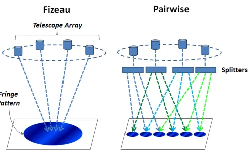
There are two popular beam combination architectures in use in optical interferometry: the pairwise combination scheme, and the Fizeau combination scheme. The two schemes are illustrated in Figure 1.1. Suppose we have a telescope array consisting ofNap apertures, each of which collectsnphotons from a distant source. In the Fizeau scheme, light from all telescopes is interfered on a single focal plane, forming an interference pattern known as afringefor each telescope pair. Each fringe encodes a sample of the scene’s 2D Fourier Transform. In the pairwise scheme, light from each aperture is splitNap ways and combined with that of each other aperture to form a single fringe pattern on separate focal planes. Hence each of the(Nap
2 )focal planes receives 2n
Nap−1 a photons, which is typically a small
fraction of the total photons incident upon the array.
Ideally an interferometer1 provides a perfect encoding of the scene’s sampled Fourier Transform. In practice, however, we never observe pristine interference fringes in either architecture. The quality of thefringesis degraded by statistical fluctuations in the arrival times of photons on the focal plane, which is a phenomenon known asshot noise. We will
Figure 1.1:The two popular beam combination schemes in optical interferometry
quantify the impact of shot noise further in the course of the thesis. For now, we note that the Fizeau architecture uses all light to form each fringe while incurring shot noise from allNapnphotons. On the other hand, the pairwise architecture uses a fraction of the light to form each fringe, which is then by corrupted by the shot noise due to the photons collected by two apertures. A fundamental result due to Zmuidzinas (2003) quantified this tradeoff and established the superior overall sensitivity of the Fizeau (or all-in-one) scheme with respect to the pairwise scheme. Because the Fizeau architecture is also typically simpler to implement, it is often preferred in practice. The results in this thesis are therefore geared toward the Fizeau architecture, although we will leverage the pairwise architecture in Chapter 4 as a conceptual springboard for subsequent analysis.
1.3
The Van-Cittert-Zernike Theorem
To derive the Theorem, let us model a source in the sky as a superposition of differential emitting elements of size ∆Ω. Consider then the electric field at the j-th aperture of an interferometric array which is a distancedfrom one such differential patch. This can be written as:
Ej(Ω) = a(ΩR)j∆Ωeiω(t−
Rj
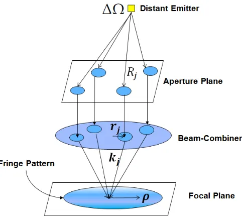
Figure 1.2:The Fizeau Interferometer Concept
wherea(Ω)is the amplitude of the field at the source, Rj is the distance from the object to thej-th aperture, ωis the angular frequency of the wave, andcis the speed of light. For
the purposes of this analysis, we neglect the amplitude variation amongst elements of the array, so that the amplitude at all apertures is a constant a(Ωd)∆Ω.
The fields from all of the point sources in the interferometer’s field-of-view are super-imposed on the system’s focal plane. For theFizeauinterferometer, this superposition is typically performed by a beam-combiner, which focuses the light collected by each aperture to a common point with propagation direction specified by an aperture-specific wave-vector
kj (see Figure 1.2).
Using the definitions above, we can compute the field contribution of each aperture at an arbitrary point on the focal planeρ. This contribution will be a function of the respective
wave-vectors and vector distances from p. Namely, we have:
Ej(ρ) = a(Ω)∆Ω
d ·e
i(kj·xj(ρ))eiω(t−Rjc) (1.2)
As we show in Appendix A.1, we can rewrite this expression in terms of the lateral aperture positionrj at the beam combiner as:
Ej(ρ) = a(Ω)∆Ω
d ·e
i(rj·ρ+φj)eiω(t−Rjc) (1.3)
whereφj is an aperture-dependent phase which is independent ofρ.
Now consider the field superposition at the pixel at vector coordinate ρ on the focal
plane (see Figure 1.2), which can be written as:
E(Ω) = a(Ωd)∆Ω·(∑Nap
j=1ei
(rj·ρ)eiω(t−Rjc)) (1.4)
where we have neglected any attenuation incurred by the field en-route to the focal plane for simplicity. To obtain the field for the complete source, we now integrate over all differential patches (which we callpoint sources) in the source to obtain:
Etotal =
Z
dΩ·a(Ω) d (
Nap
∑
j=1
ei(rj·ρ+φj)eiω(t−Rjc)) (1.5)
The detector at pixelρmeasures the intensityQof the superposition. Namely,
Q(ρ) =|Etotal|2= EtotalE∗total (1.6) or,
Q(ρ) = 1
d2
Z
dΩ1·a(Ω1)( Nap
∑
j=1
eiω(t−Rjc)ei(rj·ρ+φj))
Z
dΩ2·a∗(Ω2)( Nap
∑
k=1
e−iω(t−Rkc)e−i(rk·ρ+φk))
The final measurement is a photon count which is proportional to the time-averaged intensity. Hence, after re-arranging and time-averaging, we obtain:
hQ(ρ)i= 1
d2
Z Z
ha(Ω1)a∗(Ω2)i(
Nap
∑
j=1
eiω(t−Rjc)ei(rj·ρ+φj))(
Nap
∑
k=1
e−iω(t−Rkc )e−i(rk·ρ+φk))dΩ
Figure 1.3:Path difference between two apertures
We can simplify this expression greatly by noting that, with a few exceptions, astronomi-cal sources arespatially-incoherent, which means that the complex amplitudes of radiated waves from different points are uncorrelated. Namely,
ha(Ω1)a∗(Ω2)i = I(Ω)δ(Ω1−Ω2) (1.8) whereδ(x)denotes the Dirac delta function.
The result is that the double integral above collapses to a single integral in Ω. We can now write the sum of all pairwise products in Equation (1.7) as the following single summation over all(Nap
2 )aperture pairs: hQ(ρ)i= 1
d2
Z
I(Ω)NapdΩ+ 1
d2 Nap
∑
(j,k):k>j
(ei(ρ·∆rjk+φjk)
Z
I(Ω)ei(
ω∆Rjk
c )dΩ+e−i(ρ·∆rjk+φjk)
Z
I(Ω)e−i(
ω∆Rjk
c )dΩ) (1.9)
where the first term represents the sum of the products of each aperture’s field with its conjugate (i.e. terms of the formEjE∗j).
this unit vector would of course differ for each aperture. In most astronomical scenarios, however, the inter-aperture distance is extremely small compared with the distance between the source and the aperture array (Buscher, 2015). In such cases it is reasonable to assume that the direction vector ˆnis approximately constant across the array. As shown in Figure 1.3, we have:
∆Rjk =bjk·nˆ (1.10)
wherebjk is the vector difference position of thek-th andj-th apertures.
Moreover, we can write the differential patchdΩin terms of components of this vector
nas:
dΩ= (d2)dnxdny (1.11) Substituting Equations (1.10) and (1.11) into Equation (1.9) and noting that ω
c = 2λπ, we
obtain:
hQ(ρ)i=
Z
I(Ω)Napdnxdny+ Nap
∑
(j,k):k>j
(ei(ρ·∆rjk+φjk)
Z
I(Ω)ei(
2πbjk
λ ·nˆ)dnxdny+e−i(ρ·∆rjk+φjk)
Z
I(Ω)e−i(
2πbjk
λ ·nˆ)dnxdny) (1.12)
Note that the two integrals are F∗(bjk
λ )andF(
bjk
λ ), respectively, where F(
bjk
λ )is the 2D
Fourier Transform of the source evaluated at spatial frequency bjk
λ . For simplicity of notation,
let us index all of the aperture pairs(j,k)with a single indexh. Defining φh := φjk, and Fh := F(bλh)and substituting, we have:
hQ(ρ)i=
Z
I(Ω)Napdnxdny+
(Nap2 )
∑
h=1
Fhei(ρ·∆rh+φh)+Fh∗e−i
(ρ·∆rh+φh) (1.13)
hQ(ρ)i=F0Nap+
(Nap 2 )
∑
h=1
(orfringes), each of which encodes a distinct Fourier component of the source. This result is the Van-Cittert-Zernike Theorem which was first derived by Pieter van Cittert in 1934 (van Cittert, 1934) and then proved in simpler fashion by Frits Zernike in 1938 (Zernike, 1938).
For subsequent analysis in this thesis, it will be convenient to parameterize the fringes using the following Definitions:
Definition 1.3.1. Thecomplex fringe phasorzat a given spatial frequency is given by: z:=
|Fb|ej∠Fb
Note that the magnitude of the fringe phasor will be proportional to the brightness of the object. It is also useful to have a quantity describing the strength of a given Fourier component relative to the overall brightness of the object. This relative measure is provided by thecomplex visibility:
Definition 1.3.2. Thecomplex visibilityvof an object at a given spatial frequency is given by the ratiov= |Fh|ej∠Fh
F0
Definition 1.3.3. Thevisibilityγof an object at a given spatial frequency is the modulus of
the complex visibility, i.e. γ:= |FFh| 0
Definition 1.3.4. TheFourier phaseθof an object at a given spatial frequency is the argument
(i.e. phase) of the complex visibility, i.e. θ :=∠Fh.
With Definition 1.3.3, we can write Equation (1.15) as:
hQ(ρ)i= F0Nap+
(Nap2 )
∑
h=1
2γhF0cos(ρ·∆rh+∠Fh+φh) (1.15) The expected photon counts observed at the detectors are directly proportional to the intensity present. Let the proportionality constant relating intensity to photon counts be given byκ, so that a vectorized representation of these expected photon counts is given by:
hy(ρ)i=κF0Nap+κ (Nap2 )
∑
h=1
Moreover we assume that light is conserved throughout the fringe generation process, and hence the photon counts must sum to the total numberTp of photons incident upon the array, i.e.Tp =nNap, i.e.
Tp=
∑
ρ
hy(ρ)i=
∑
ρ
κF0Nap+κ
(Nap2 )
∑
h=1
2γhF0cos(ρ·∆rh+∠Fh+φh)
=nNap (1.17)
In this thesis, we will consider the scenario in which the periods of the fringe sinusoids are all integer multiples of pixels on the focal plane. This is one of the so-called DFT conditionscommonly employed in interferometry to avoid fringe estimation bias due to spectral leakage (Gordon, J. A. and Buscher, D. F., 2012). In this case the sinusoidal term vanishes in the sum in Equation (1.17) leaving only the constant (first) term, and if we define Nf p as the number of pixels on one side of a square focal plane, we have:
∑
ρ
κF0Nap = N2f pκF0Nap =nNap (1.18) which in turn implies that κ = Fn
0N2f p
, and hence by substitution into Equation (1.16) yields:
hy(ρ)i= nNap
N2f p + 2n N2f p
(Nap2 )
∑
h=1
γhcos(ρ·∆rh+θh+φh) (1.19)
1.4
The Cramer-Rao Bound for the Complex Visibilities
There are two principal sources of noise that affect this measurement. We have already alluded to theshot noisearising from the fact that photon arrivals are not uniform in time even if incident intensity is constant. The resulting uncertainty in photon counts for a given exposure time is well-modeled as a Poisson distribution with meanλT, where λis
not, the former dominates the latter in high light-level scenarios. And with recent advances in electronics, the light-level regime in which read noise is important continues to diminish. We will therefore focus on detection limits for the shot-noise-limited case.
Recall Equation (1.19) provides an expression for the time-averaged intensity. To obtain lower bounds on sensitivity, let us assume that the phase differences∆θh are known and therefore calibrated. We can write the observation model in matrix form as:
hy(ρ)i= nNap
N2 f p + 2n N2 f p ... ×
cos(ρ(1)·∆k1) −sin(ρ(1)·∆k1) cos(ρ(1)·∆k2) −sin(ρ(1)·∆k2) ... cos(ρ(2)·∆k1) −sin(ρ(2)·∆k1) cos(ρ(2)·∆k2) −sin(ρ(2)·∆k2) ...
...
Re[v1] Im[v1] Re[v2] Im[v2]
...
Suppose that the interferometer’s output is a beam with an extent of Nf p pixels on the focal plane. LettingAbe the N2
f p-by-2( Nap
2 )matrix in the equation above (the so-called visibility-to-pixel matrix(V2PM)), we can write this matrix equation compactly as:
y= nNap
N2 f p
1T Nf p+
2n N2 f p
Avˆ (1.20)
where1TNf p denote the constantonesvector of length Nf p, ˆvis the vector containing the quadrature components of the complex visibilities. The actual pixel counts can be modeled as i.i.d. Poisson random variables with meansy, i.e.
Y∼Poisson(y). (1.21)
p(Y|y) =
Nf p
∏
i=1
(eiTy)Yi
Yi!
exp(−eiTy) (1.22) whereei is the unit vector of thei-th canonical basis. Substituting fory, we obtain the negative log-likelihood as:
F(y) =1TN
f py−
Nf p
∑
i=1
Yilog(eTi y) +C (1.23) where 1 is an all-ones vector of size Nf p, andC is a constant independent of ˆv. Let ˜
A:= 2n
N2 f p
A. Then the gradient with respect to ˆvis given by:
∇vˆF(y) =A˜T1− Nf p
∑
i=1 Yi eTi yA˜
Te
i (1.24)
Therefore the Hessian is:
∇2 ˆ
vF(y) =A˜T Nf p
∑
i=1 Yi
(eiTy)2eie
T
i A˜ (1.25)
To obtain the Fisher information matrixI(ˆv), we take the negative-expectation of this quantity:
I(ˆv) =−E[∇v2ˆF(y)] =−A˜T
Nf p
∑
i=1 E[Yi]
(eT i y)
2eie T
i A˜ (1.26)
But since E[Yi] =eiTy, this simplifies to:
I(ˆv) =A˜TDA˜ (1.27)
whereDis a diagonal matrix withDii = (eT1 iy).
Figure 1.4:The relationship between aperture patterns and Fourier sampling
var(vˆi)≥[I(ˆv)−1]ii (1.28) This expression matches the result given by Zmuidzinas (2003).
1.5
Key Parameters of an Interferometer: Resolution, Field-of-View,
and Undersampling Ratio
In the Section 1.3 we established that the interference fringe generated by a pair of apertures separated by a vector b encodes the amplitude and phase of the Fourier Transform of the scene at spatial frequency bλ. For real images each baseline actually contributes two spatial frequency samples, as the Fourier Transform of real images is conjugate symmetric. As an example, consider the aperture pattern in the left panel of Figure 1.4. Suppose we are interfering light at a wavelength of 500 nm. The baseline b12 formed by apertures 1 and 2 generates a fringe encoding the complex visibility v12 at a spatial frequency of
b12
λ = (2e6, 6e6) cycles/radian, and its conjugate v
∗
12 at a spatial frequency −(2e6, 6e6) cycles/radian.
Figure 1.5:Representation of a scene as a Field-of-View comprised of resolution elements
in Figure. Suppose we sample a 2D-signal in the Fourier domain with sampling interval
∆s,f req = 2R1 along each dimension. By the well-known Nyquist Sampling Theorem, we know that only images spatially-limited to±Ralong each dimension can be uniquely represented with these samples; images beyond this extent will suffer from aliasing. Therefore an interferometer whose sampled spatial frequencies lie on a grid with spacing∆min = bminλ has an unambiguous Field-of-View area of ∆21
min
= λ2
b2 min
. Conversely, by the space-frequency duality of the Nyquist Theorem, we know that we can uniquely represent an image ban-dlimited to frequency extent±Lby sampling in space at an interval of∆s,space = 2L1. Given the maximum spatial frequency observed by our interferometer is L = ∆max = bmax
λ , the
bandlimited approximation of the image is uniquely defined by samples spaced λ
2bmax apart
along each dimension. Therefore the size of the smallest resolvable element in the image, which we call the resolution element, is given by λ2
4b2
max. Figure 1.5 depicts the notions of
Field-of-View (FOV) and resolution element (resEl) visually.
With the areas of the Field-of-View and resolution element in hand, we can now compute the number of resolution elements in the bandlimited approximation of the image as the ratio of these two quantities, or:
wherer = bmax
bmin.
We now define our undersampling ρ as the ratio of the number of distinct Fourier
samples to the number of resolution elementsNresEls in the image. Each Fourier sample we measure is actually a pair of samples since for real images, the value of the Fourier Transform at a given spatial frequency is the conjugate of that at the corresponding negative spatial frequency. Hence we have:
ρ= 2
(Nap
2 ) NresEls
= 1
2r2
Nap 2
(1.30)
1.6
Atmospheric and Instrumental Phase Noise
Our analysis thus far has assumed that the effective path between the beam-combiner and the target depends merely on the source-instrument geometry depicted in Figure 1.2. In practice there are several deterministic and random sources of path variation across the aperture array. Common deterministic sources of path variation include that in the optical paths traversed between the instrument’s front-end and beam-combiner. The predominant random sources of delay are atmospheric turbulence and instrumental vibration. Atmospheric turbulence, which is typically the more stressing of these two sources, alters the optical path traversed by the wave arriving at each aperture in a nonuniform and time-varying manner.
Let us consider the total path alteration due to all of the sources mentioned. Let us then define the corresponding phase shift resulting from this alteration at aperturejaseiφj,total. If
these phase shifts are carried through the analysis in Section 1.3, we obtain:
hy(ρ)i= nNap
N2 f p
+ 2n
N2 f p
(Nap2 )
∑
(j,k)
γjkcos(ρ·∆rjk+θjk+φjk) (1.31) whereφjk := φj,total−φk,total is the difference between the total phase shifts at the two
apertures in the baseline associated with aperture pair(i,j).
wave-lengths. Suppose the atmosphere adds phasesφj andφk to apertureskand j, respectively. The result is that the observed complex visibility is given by:
˜
vjk=vjkei(φj−φk) (1.32) We can eliminate such nuisance factors by forming a triple product g of the Fourier phasors along a triangle of baselines (e.g. g123 := v˜12v˜23v˜31). As shown in Figure 1.6, this special triple product (known as thebispectrum) cancels the atmospheric phase terms, leaving only the desired Fourier information (i.e. the{θ}). The phase of the bispectrum
∠g, which is known as the closure phase, can hence be used to recover estimates for the Fourier phases. Consider an interferometer that measures all baselines amongNap apertures. Out of the(Nap
3 )possible triangles, only ( Nap−1
2 )of the associated closure phase relations are linearly-independent (Readheadet al., 1988). If we combine these closure phases with the Fourier magnitude estimates for each of the (Nap
Chapter 2
Leveraging compressed sensing
techniques in optical interferometry
2.1
Citation to Previously-Published Work
This chapter contains text and figures published previously in the following paper:
Kurien, B. G., Rachlin, Y., Shah, V. N., Ashcom, J. B. and Tarokh, V. (2014). Compressed sensing techniques for image reconstruction in optical interferometry. In Imaging and Applied Optics 2014, Optical Society of America, p. SM2F.3.
2.2
Chapter Overview
directly apply. We have developed and validated a robust algorithmic interface between the Fourier magnitude and bispectrum observables available in the optical interferometry and SR regularizations known as Total Variation Minimization for which fast solvers exist.
2.3
Problem Statement and Approach
There are two principal challenges that one encounters when trying to reconstruct im-ages from optical interferometric measurements. Each aperture pair (or baseline) in an interferometer samples the Fourier transform of the image in its field of view at a spa-tial frequency bλ, where b is the length of the baseline, and λ is the wavelength of light
collected. Interferometers rarely measure enough baselines to fully sample the Fourier transform. Hence reconstruction of the image from such undersampled measurement set is an ill-posed (or underdetermined) problem; we must recover intensities for NresEl resolution elements in the scene under observation fromm NresEl spatial frequency measurements corresponding to the available baseline pairs in the telescope array. To make the problem well-posed, additional constraints must be enforced. Traditionally regularization approaches based on the so-calledCLEAN algorithm due to Högbom (1974), which implicitly fits the measurements to an image model consisting of a sparse collection of point-like sources, have been used to solve this problem.
It is well-known in imaging that successful regularization schemes apply constraints which accurately capture the properties of the image we wish to reconstruct. Likewise the success of the CLEAN algorithm has been largely limited to astronomical scenes which closely match its point-source-collection assumption. The astronomical community has hence been led to consider more generally-applicable prior models. A property shared by an overwhelmingly-large fraction of natural images iscompressibility. Compressible images are those which can be well-approximated by a sparse representation in some domain. The smallness of an image’s L1-norm1, as applied to either directly to the image pixels, their
1The L1-norm of a vectorized imagex, denotedkxk
gradient, or their wavelet coefficients, has proven to be a remarkably effective proxy for the image’s compressibility. This observation and techniques that exploit it are at the core of the field ofsparse recovery(SR) as well as the tightly-linked field ofcompressed sensing(CS) (Candèset al., 2006) (Donoho, 2006). Though a wide variety of sparse-recovery techniques have arisen in the past few decades, the vast majority of them regularize problems with a linear observation model:
y=Fx+n (2.1)
where yis the measurement vector,x is a vector representing the unknown signal or image,Fis the measurement matrix, andnrepresents additive measurement noise.
While sparse-recovery techniques have been applied successfully to reconstruction in radio interferometry (Wiaux et al., 2009), optical interferometry, on the other hand, poses additional challenges beyond the Fourier-undersampling problem discussed above. Namely, atmospheric turbulence necessitates a non-linear formulation of the reconstruction problem. Recall from Chapter 1 that there are (Nap
2 )unknown Fourier phases as well as Nap−1 unknown piston differences, and hence inference of the Fourier phases from the
(Nap
frame).
In Section 1.6 we introduced the bispectrum observable as the classical basis for atmosphere-invariant inference in optical interferometry. Formed as the product of three fringe phasors associated with the sides of a baseline triangle (e.g. b12, b23, and b31), the bispectrum is a non-linear function of the complex visibilities of the image. Recall that the atmosphere-induced terms cancel in these products and hence, like the Fourier magnitudes, these so-calledbispectraare atmosphere-invariant observables. However, for a non-redundant array with(N2)distinct baselines, recovery of the Fourier phases from the bispectra phases (i.e. theclosure phases) remains ill-posed since there are only(N−21) indepen-dent closure phases (Readheadet al., 1988). Successful bispectra-based image reconstruction remains feasible in spite of this ill-posedness (see e.g. Thiébaut (2013), Besneraiset al.(2008)), but again prior constraints (e.g. on the image support) must be enforced to regularize the reconstruction.
An important property of the bispectrum which we will exploit in our reconstruction method is its invariance to scene translation. To illustrate this property, let us denote the spatial frequency vectors of two sides of a bispectrum triangle as u and v, respectively. Then the spatial frequency of the remaining side will be w := −(u+v). If ˆg(p) is the corresponding (normalized) bispectrum of a scene at its original position p, then by the shift property of the Fourier transform, the bispectrum of the translated image becomes:
ˆ
g(p+δp) =ej(θu+u·δp)ej(θv+v·δp)ej(θ−(u+v)−(u+v)·δp) (2.2)
=ej(θu+θv+θ−(u+v))= gˆ(p) (2.3) where we have dropped the aperture subscripts for purposes of generality.
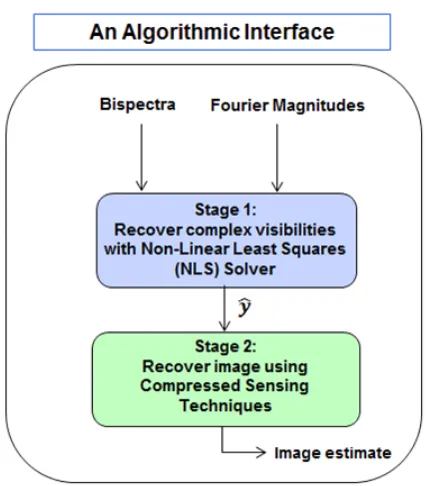
Figure 2.1:Overview of Proposed Two-Stage Approach
With the Fourier component estimates at hand, the image estimate can then be recovered using standard SR techniques. The approach is diagrammed in Figure 2.1 below.
2.4
Description of Stage 1 of Algorithm
The goal of Stage 1 of our algorithm is to use the measured bispectra and Fourier magnitudes to recover estimates of the true Fourier components of the image. Recall from Section 1.3 that the fringes provide measurements of the Fourier magnitudes directly. Hence it remains to recover the Fourier phase information. Since there are(Nap
2 )unknown Fourier phases in a non-redundant array but only(Nap−1
to a spatially-compact intensity profile in the image domain. This kind of joint metric has been suggested for optical interferometric applications before in the work of Thiébaut (2013). However, whereas the method in Thiébaut (2013) searches for a metric-minimizing image, our method first searches for the metric-minimizing baseline phase set, which is inherently a smaller set given the undersampled nature of the problem.
ˆ
θ=arg min
θ
fdata(θ, ¯g,a) +µfprior(θ,a) (2.4)
The data (orresidual) and prior terms are defined as follows.
fdata(θ, ¯g,a) =
Nb
∑
k=1
1 wk
(g¯k−ak1ak2ak3exp(j(θk1+θk2+θk3)))
2
(2.5) where ¯gk is thek-th bispectrum measurement,{θki}are the unknown Fourier phases in
thek-th bispectrum, the{aki}are estimates for the magnitudes of the Fourier coefficients in thek-th bispectrum, andwk is a weighting factor proportional to the estimated variance of thek-th bispectrum.
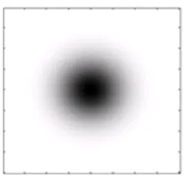
fprior(θ,a) =Re[F∗ya,θ](1−hgaussian)
2
(2.6) whereFis the partial DFT matrix whose rows are 2D-sinusoidal basis functions sampled by the array,ya,θis the vector of estimated Fourier coefficients with magnitudes given bya
and phases given byθ,hgaussian denotes a centered Gaussian window with a peak value of unity,1denotes the vector whose entries are all 1, and the operationdenotes point-wise multiplication.
An intuitive interpretation of the regularization above can be obtained by decomposing the computation into steps. We seek to fit the bispectra with a set of Fourier phases ˆθwhich
together with the estimated Fourier magnitudes produce an image with compact energy. The data term in the metricfdatais a sum of the squared residuals of measured bispectra with respect to the bispectra associated with the phase vector ˆθ. The steps for computation
Figure 2.2:Inverted Gaussian penalty function 1−hgaussian
; the dark region represents an area of near-zero penalty
magnitude estimates inato form estimates for the complex Fourier componentsya,θ. We
then apply the pseudo-inverse of the partial DFT matrixFto the vector ya,θand retain the
real part2, thereby obtaining an image-space representation ofya,θ. Finally, we perform
point-wise multiplication of this image with a function of the form shown in Figure and compute the norm of the result. This operation computes a compactness metric which penalizesya,θin proportion to its spatial energy spread. Note that the actual position of the
Gaussian taper is immaterial; as established above, the bispectrum is a translation-invariant quantity and hence the joint metric will be invariant to shifts of the same object.
The joint data-prior metric in Equation (2.4) can be minimized using a suitable non-linear least-squares solver. For our processing, we have elected to use the MATLABr implementation (MATLAB, 2012) of the trust-region reflective non-linear least-squares solver.
2.5
Description of Stage 2 of Algorithm
Stage 2 takes the Fourier estimates obtained in Stage 1 and attempts to recover an image using fast sparse-recovery (SR) techniques. This amounts to solving the linear, under-determined inference problem:
ˆ
y=Fx˜ +n (2.7)
where ˆyis the vector of Fourier estimates from Stage 1, ˜Fis the partial-DFT matrix whose rows are the complex-sinusoidal basis functions corresponding to the spatial frequencies sampled by the array3, and n is the (unknown) residual error in these estimates. Since in practice there are fewer available Fourier measurements than the desired number of resolution elements in the image, this inference problem is ill-posed from a Nyquist-sampling perspective. Hence once again we must regularize the problem by imposing constraints on the image. We selected two different SR regularization strategies due to their widespread success in solving similar inverse problems involving Fourier undersampling. The first of these approaches, Basis Pursuit Denoising (BPDN), seeks to find the image of smallest L1-norm which also agrees with the estimated Fourier component estimates to within a certain tolerancee. We performed this L1-minimization in the wavelet domain as opposed
to the pixel domain, as it is well-known that natural images tend to be more compressible in the former domain than in the latter. The other regularization we tested, Total Variation Minimization (TV-Min), is very similar, but seeks instead to minimize another quantity known to be compressible in natural images: the L1-norm of the gradient of the image. The two regularization techniques are specified mathematically below:
(Basis Pursuit Denoising): ˆx=arg min
α
kαk1subject to:
FΨ
−1
α−yˆ
2≤e (2.8)
(Total Variation Minimization): ˆx=arg min
α
kαkTVsubject to:kFα−yˆk2≤ e (2.9)
where kαkTV is the L1-norm of the 2D pixel gradient of the image, i.e. kαkTV :=
∑i,jk∇α[i,j]k1.
3Note that ˜Fneed not be the same asF, as we are free to assume an independent pixel resolution in each
The software package NESTA (Becker et al., 2011) was used to perform the Stage 2 optimizations above.
2.6
Algorithm Performance
2.6.1 Laboratory Validation
To test the effectiveness of our algorithm when applied to real interferometric data, we collected fringe data with MIT Lincoln Laboratory’s (MIT/LL) Fizeau Interferometer. The interferometer is a reconfigurable fiber-coupled system that allows all(202)baseline conjugate pairs to be measured simultaneously by projecting light from all apertures onto a Fizeau beam-combiner. For our experiments, we used a 20-aperture compact, non-redundant pattern of the Golay type (Golay, 1970). The pattern is shown in Figure 2.3. The ratio r of the maximum baseline to the minimum baseline was 17 in both x and y spatial coordinates. Hence the number of resolution elements required to uniquely specify our diffraction-limited scene was(2r)2, yielding an undersampling ratio ofρ= 2∗190
(2∗17)2 ≈0.33.
The interferometer was illuminated with the far-field projection of a range of targets: chrome-on-glass transparency masks were photolithographically-prepared and placed at the focus of an 12f three-mirror off-axis telescope. When the target is illuminated with the white light, the far-field projection of the target is produced at the telescope aperture, where it can be sampled. As a reference for reconstruction, we consider a reduction of the actual target to the fundamental diffraction-limited resolution of the instrument as shown in Figure 2.4.
5000-frame reconstruction results are shown in Figure 2.5 for the following photoelectron (pe) levels: (from left to right) 320e3 pe/aperture/frame, 54e3 pe/aperture/frame, and 15e3 pe/aperture/frame.
2.6.2 Simulation
Figure 2.3:Non-redundant Golay 20-aperture pattern (left) and corresponding UV-sampling (right)
Figure 2.4:Target chrome mask (left) and corresponding truth image at diffraction-limited resolution (right)
Figure 2.6: Image Reconstruction Results from Simulations
atmospheric distortion against that if this distortion were known. Note that in the latter atmosphere-oraclecase, bispectrum formation is not required and direct SR reconstruction from complex amplitudes is feasible. Hence this comparison allows a quantitative measure of the reconstruction penalty suffered from bispectrum formation. Our comparative simulation scheme is depicted in the block diagram in Figure 2.6.
We used two Image Quality Metrics to assess performance: the standard metric Normal-ized Mean-Squared Error (NMSE) and the Structural Similarity (SSIM) metric (Wanget al., 2004). The NMSE is defined as:
N MSE=20 logkxˆ−x0k
x0
Figure 2.7: Image Reconstruction Results from Simulations
Figure 2.8:Algorithm Performance in Simulation
Chapter 3
Pattern design criteria for uniqueness
in phase recovery
3.1
Citation to Work under Review
This chapter contains text and figures submitted for publication to the Monthly Notices of the Royal Astronomical Society (MNRAS).
Kurien, B., Tarokh, V., Ashcom, J., Rachlin, Y. and Shah, V. (2016). Resolving phase ambiguities in the calibration of redundant interferometric arrays: implications for array design. Monthly Notices of the Royal Astronomical Society, (submitted, March 4, 2016)
3.2
Chapter Overview
reconstruction. In this paper, we show that these ambiguities affect recently-developed RSC phasor-based reconstruction approaches operating on the complex visibilities, as well as traditional phase-based approaches operating on their logarithm. We also derive new sufficient conditions for an interferometric array to be immune to these ambiguities in the sense that their effect can be rendered benign in image reconstruction. This property, which we callwrap-invariance, has implications for the reliability of imaging via classical three-baseline phase closures as well as generalized closures. We show that wrap-invariance is conferred upon arrays whose interferometric graph satisfies a certain cycle-free condition. For cases in which this condition is not satisfied, a simple algorithm is provided for identifying those graph cycles which prevent its satisfaction. We apply this algorithm to diagnose and correct a member of a pattern family popular in the literature.
Before we discuss phase-wrapping ambiguities, we first review a few key preliminary mathematical notions from lattice theory in the next Section.
3.3
Preliminaries
3.3.1 Lattices
Alattice is a mathematical object describing a repeating pattern of discrete points in space. It arises in a variety of scientific and engineering contexts including crystallography and communication theory. We will define a latticeΛas a linear combination of vectors in which the coefficients are integers, i.e.
Λ=
(
m
∑
i=1
aivi | ∀ai ∈Z
)
Many lattice algorithms, including algorithms for the Closest Vector Problem introduced in the next section, require areducedlattice basis. Areducedbasis is one consisting of vectors which are short and nearly-orthogonal. A well-known procedure to create a basis for a given lattice with short, nearly-orthogonal vectors is known as theLLLalgorithm due to Lenstraet al.(1982).
An LLL-based routine for forming a reduced lattice basis from a set of generating vectors which are not necessarily linearly-independent is given in Cohen (1993).
3.3.2 The Closest-Vector-Problem
A well-known problem in lattice theory is theClosest-Vector-Problem, which can be described as follows:
Problem 3.3.1. Given a basis {b1,b2, ...,bn}for a lattice inRm and a vectorw∈ Rm, find the point in the lattice closest in Euclidean distance fromw.
Several algorithms exist for solving this problem. A popular class of algorithms, known as the Sphere-Decoding algorithms, are efficient searches for the closest lattice point within a hypersphere of a certain radius centered on the input vector (see e.g. Agrellet al.(2002)). For the simulations in this chapter, we instead use the lower-complexity Babai Nearest Plane (Babai-NP) algorithm (Babai, 1986). For lattice bases which are nearly orthogonal, this algorithm offers reliable, albeit not guaranteed, performance in practice. Pseudo-code for one implementation of this algorithm due to Galbraith (2012) is given in listing Algorithm 1.
Algorithm 1Babai Nearest-Plane Algorithm
Input: Basis for latticeΛ(i.e. {b1, . . . ,bn}), andw∈Rm
Output: Elementv∗ nearest towinΛ
Compute orthogonal basis{b∗1, . . . ,b∗n}using Gram-Schmidt procedure
fori=n downto 1 do
Setli = hwi,b
∗ ii
hb∗i,b∗ii Setyi =bliebi
Setwi−1=wi−(li− blie)b∗i − bliebi
end for
A conceptual interpretation of this recursive algorithm is as follows. At the root level, the algorithm finds the vector inΛclosest to w; in other words it solves the CVP problem
(Λn,w). First consider the subspaceU spanned by the firstn−1 basis vectors, i.e. U =
span{b1, . . . ,bn−1}. The algorithm begins by computing the translatey ∈ ΛofUclosest tow, i.e. the nearest plane to w. The algorithm then implicitly computes the projection
w0 of w onto this translate U+y. It then translates this projection back to the origin (i.e. wn−1 := w0−y), and solves the smaller problem within U, i.e. the CVP problem
(Λn−1,wn−1), whereΛn−1 is the lattice formed by the firstn−1 basis vectors. The process continues recursively until the final CVP problem with the lattice spanned byb1is solved. The final output is then the sum of the translates from each level of the recursion.
3.4
Problem Statement and Related Work
5 10 15 20 25 30 35 40 45 50 0.02
0.04 0.06 0.08 0.1 0.12 0.14 0.16 0.18 0.2 0.22
Aperture Count
[image:55.612.168.439.98.298.2]Required redundant fraction
Figure 3.1:Fraction of redundant baselines required for critical redundancy vs. aperture count
focal plane has long been a popular method of acquiring many baseline measurements in an economical manner. However, the Fizeau method had been incompatible with RSC techniques since the fringes formed by each set redundant baselines would alias on the focal plane. An elegant solution to this problem was proposed by Perrinet al.(2006). This work developed the idea of segmenting the entrance pupil of a single telescope into an RSC arrangement of sub-pupils from which the light was then coupled via single mode fiber to a non-redundant exit pupil, thereby permitting unambiguous and simultaneous fringe detection for an RSC array. A reconstruction algorithm for this architecture was then proposed in Lacouret al.(2007). Even more recently, RSC has been implemented as the calibration scheme of choice for several radio interferometers: the Donald C. Backer Precision Array for Probing the Epoch of Reionization (PAPER) in South Africa (see Ali et al.(2015)), the MIT Epoch of Reionization (MITeOR) in the United States (see Zhenget al. (2014)), and the Ooty Radio Telescope (ORT) in India (see Marthi and Chengalur (2014)).
unique spatial frequencies measured by the interferometer. However, as Figure 3.1 illustrates, the fraction of distinct uv-samples sacrificed for critical redundancy becomes increasingly negligible as the number of apertures in the array increases. Nevertheless the RSC technique presents other challenges which must be overcome for reliable imaging. Central among these challenges is the problem of integer phase ambiguities which arise from the fact that the interferometric phase is only known modulo 2π. Indeed these ambiguities have been
shown to play an important role in accurately recovering sensor complex gains and object complex visibilities while imaging with real interferometric instruments (see e.g. Liuet al. (2014), Eastwoodet al.(2009)). In this chapter, we describe these ambiguities and how they can be mitigated using a combination of lattice theory algorithms and careful array design. We will see that these ambiguities have a fundamental presence; namely, they exist whether the calibration strategy works with complex visibilities (which we call thePhasorapproach) directly, or their respective logarithms (which we call thePhaseapproach). To the best of our knowledge, the results in this chapter are the first to provide array conditions allowing unambiguous interferometric phase determination in spite of wrap ambiguities in the Phase approach, and corresponding false minima in the objective of the Phasor approach.
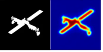
To motivate the analysis in the chapter, we provide an example illustrating the effect that wrap ambiguities can have in RSC-based image reconstruction. Consider the pattern depicted in the Figure 3.2. This pattern belongs to one of the more popular array classes in the interferometry literature: the so-calledY-patterns(see e.g. Arnotet al.(1985), Blanchard et al.(1996), Labeyrieet al.(2006), Eastwoodet al.(2009), Liuet al.(2014)). The corresponding spatial, orUV, sampling is provided in the right panel of the Figure.
Figure 3.2: Y-pattern Array Example
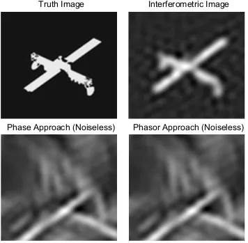
by Lannes (2003), and the lower right panel shows the same for an implementation of the Phasor method (Marthi and Chengalur, 2014) (Lacouret al., 2007). Reconstruction suffers from phase wrapping error in the former case, and a corresponding false-minimum trap in the Phasor case. In the course of this chapter, we will first identify this ambiguity from a mathematical perspective, relate it to a particular physical structure (i.e. the existence of a certain type of loop in the interferometric graph), and provide a simple algorithm for identifying such structures in an arbitrary array so that they can be remedied.
The chapter is organized as follows. In Section 3.5, we review previous work on the integer ambiguity problem, and discuss its presence in the Phase approach. We provide new mathematical conditions for an aperture pattern to bewrap-invariant, meaning that the effect of the 2π-periodicity of the measured interferometric phase can be eliminated