hypernova explosions
.
White Rose Research Online URL for this paper:
http://eprints.whiterose.ac.uk/97642/
Version: Published Version
Article:
Barkov, MV and Komissarov, SS (2011) Recycling of neutron stars in common envelopes
and hypernova explosions. Monthly Notices of the Royal Astronomical Society, 415 (1). pp.
944-958. ISSN 1365-2966
https://doi.org/10.1111/j.1365-2966.2011.18762.x
This article has been accepted for publication in Monthly Notices of the Royal Astronomical
Society ©: 2011 Author(s) Published by Oxford University Press on behalf of the Royal
Astronomical Society. All rights reserved
[email protected]
https://eprints.whiterose.ac.uk/
Reuse
Items deposited in White Rose Research Online are protected by copyright, with all rights reserved unless
indicated otherwise. They may be downloaded and/or printed for private study, or other acts as permitted by
national copyright laws. The publisher or other rights holders may allow further reproduction and re-use of
the full text version. This is indicated by the licence information on the White Rose Research Online record
for the item.
Takedown
If you consider content in White Rose Research Online to be in breach of UK law, please notify us by
Recycling of neutron stars in common envelopes and hypernova explosions
Maxim V. Barkov
1,2,3⋆
and Serguei S. Komissarov
2⋆
1Max-Planck-Institut f¨ur Kernphysik, Saupfercheckweg 1, 69117 Heidelberg, Germany 2Department of Applied Mathematics, The University of Leeds, Leeds LS2 9JT 3Space Research Institute, 84/32 Profsoyuznaya Street, Moscow 117997, Russia
Accepted 2011 March 21. Received 2011 March 14; in original form 2010 December 22
A B S T R A C T
In this paper, we propose a new plausible mechanism of supernova explosions specific to close binary systems. The starting point is the common envelope phase in the evolution of a binary consisting of a red supergiant and a neutron star. As the neutron star spirals towards the centre of its companion it spins up via disc accretion. Depending on the specific angular momentum of the gas captured by the neutron star via the Bondi–Hoyle mechanism, it may reach millisecond periods either when it is still inside the common envelope or after it has merged with the companion core. The high accretion rate may result in the strong differential rotation of the neutron star and generation of the magnetar-strength magnetic field. The magnetar wind can blow away the common envelope if its magnetic field is as strong as 1015G and can destroy the entire companion if it is as strong as 1016G. The total explosion energy can be comparable to the rotational energy of a millisecond pulsar and reach 1052erg. However, only a small amount of56Ni is expected to be produced this way. The result is an unusual Type II supernova with very high luminosity during the plateau phase, followed by a sharp drop in brightness and a steep light-curve tail. The remnant is either a solitary magnetar or a close binary involving a Wolf–Rayet star and a magnetar. When this Wolf–Rayet star explodes, it will be a third supernova explosion in the same binary.
Key words: stars: magnetars – stars: neutron – supernovae: general.
1 I N T R O D U C T I O N
Usually, neutron stars (NSs) have magnetic fieldB∼1012G and
rotate with a period of a fraction of a second, the Crab pulsar being a typical example. However, we now know that the ‘zoo’ of NSs is much more diverse and they can have both much weaker and much stronger magnetic field and rotate with both much longer and much shorter periods.
Around 10 per cent of NSs have the surface dipolar magnetic field
B∼1014–1015G (Kouveliotou et al. 1998). These ‘magnetars’ are
believed to be born in core-collapse explosions of rapidly rotating stars. During the collapse, the proto-NS naturally develops strong differential rotation, which allows for the generation of magnetic field viaα–dynamo (Duncan & Thompson 1992; Thompson & Duncan 1993). The strength of the saturated magnetic field strongly depends on the rotational period, with shorter periods leading to stronger magnetic field and more rapid release of rotational energy. In order to generate the magnetar-strength magnetic field, the rota-tion period must be around few milliseconds (Duncan & Thompson 1992). Such a strong field allows to release up to 1052erg of the
⋆E-mail: [email protected] (MVB); [email protected]
(SSK)
magnetar’s rotational energy in very short period of time. This is sufficient to drive extremely powerful supernova explosions, on the hypernova scale, and to produce powerful gamma-ray bursts (GRBs, e.g. Usov 1992; Thompson, Chang & Quataert 2004). The turbulence required for the magnetic dynamo action can also be generated via the magnetorotational instability (Balbus & Hawley 1991). Calculations based on the linear theory show that in the su-pernova context strong saturation field can be reached very quickly on the time-scale of only several tens of rotational periods (Akiyama et al. 2003; Obergaulinger et al. 2009).
Millisecond pulsars are found in low-mass binaries, and it is gen-erally thought that they have been spun up via disc accretion (Alpar et al. 1982; Archibald et al. 2009). This origin implies mass increase by about 0.2 M⊙compared to normal radio pulsars, whose masses are narrowly distributed around 1.35 M⊙(Thorsett & Chakrabarty 1999). It is rather difficult to measure the mass of a millisecond pulsar, but the few available results agree with this prediction of the accretion model (Kaspi, Taylor & Ryba 1994; Jacoby et al. 2005; Demorest et al. 2010). The most massive pulsar found to date, al-most 2 M⊙, is a millisecond pulsar (Demorest et al. 2010). The magnetic field of these millisecond pulsars is very low, down to 109
G. Most likely, their initial magnetic field was of similar strength to normal pulsars, but now it is buried under the layers of accreted matter (Bisnovatyi-Kogan & Komberg 1974; Alpar et al. 1982).
at University of Leeds on April 1, 2016
http://mnras.oxfordjournals.org/
The reason why these pulsars could not generate magnetar-strength magnetic field in the same way as in the core-collapse scenario is the very long time-scale of spinning up compared with the viscous time-scale. As a result, the differential rotation remains weak and there is not enough energy for effective magnetic dynamo (Spruit 1999).
The rotational frequency of the fastest X-ray pulsar is∼760 Hz (Chakrabarty et al. 2003), whereas the fastest known radio pulsar has the frequency of 641 Hz (Backer et al. 1982). Most likely, it is the gravitational radiation loss what places the upper limit on the rotation rates because at high spin the r-mode oscillations become excited (Shapiro & Teukolsky 1983; Levin 1999). Spruit (1999) ar-gued that this instability may also result in magnetic explosions. The idea is that the heating of NSs, associated with these oscillations, reduces their viscosity and decouples its interior from the outer lay-ers. Being most disturbed, the outer layers rapidly lose some of their angular momentum via gravitational radiation. This leads to strong differential rotation and the generation of the magnetar-strength magnetic field in the NS interior. This field becomes unstable to buoyancy, emerges on the surface, and the magnetically driven pul-sar wind rapidly extracts the rotational energy of the NS. Spruit (1999) proposed this as an alternative scenario for long GRBs. It is unlikely that a supernova-like event can accompany a GRB in this scenario. Although the wind energetics are sufficient, only a small fraction of this energy can be deposited into the companion star, simply because of its small geometrical cross-section. Moreover, recent results suggest that the amplitude of r modes may satu-rate at a much lower level due to non-linear interaction with other modes (Arras et al. 2003; Brink, Teukolsky & Wasserman 2005; Bondarescu, Teukolsky & Wasserman 2007).
A similar recycling of NSs may occur during the common-envelop (CE) phase, after the primary becomes a red super-giant (RSG; Bisnovatyi-Kogan & Syunyaev 1971; Paczynski 1976; Tutukov & Yungelson 1979; Postnov & Yungelson 2006). Due to the dynamic friction, the NS then spirals inside the RSG, accret-ing on its way. Now one can imagine two interestaccret-ing outcomes of such processes. First, the NS may accumulate too much mass and collapse into a black hole (BH). This BH is likely to be rapidly ro-tating and drive a stellar explosion in the collapsar fashion (Fryer & Woosley 1998; Zhang & Fryer 2001; Barkov & Komissarov 2010). Secondly, the NS may first spin up to a millisecond period and drive a magnetic explosion of the type proposed by Spruit (1999) but now inside the CE. The magnetar wind can keep energizing such supernovae, producing a similar effect to radioactive decay (Kasen & Bildsten 2010; Woosley 2010). High accretion rates may modify the way the NS is recycled. The accreted gas can form a massive rapidly rotating layer above the NS crust (Inogamov & Sunyaev 1999, 2010). The strong differential rotation between the layer and the NS core may result in the development of the Kelvin–Helmholtz instability when the NS crust melts down under the weight of the layer. This may lead to the turbulence and strong amplification of the NS magnetic field.
The accretion on to NSs during the in-spiral has been studied by Chevalier (1996) who concluded that the high angular momentum of the gas gravitationally captured by a NS prevents it from effective neutrino cooling and keeps the mass-accreting rate well below the rate of the Bondi–Hoyle capture. As a result, the NS accumulates very little mass while still inside the CE. On the other hand, he suggested that during the merger with the companion core the mass accretion rate rises and the NS collapses into a BH. While carefully analysing various effects of rotation, Chevalier (1996) did not use any particular model for the primary. Moreover, there is a great
deal of uncertainty as regards the specific angular momentum of the gravitationally captured gas. In our study, we come back to this problem, consider realistic models of RSG stars and allow for the uncertainty.
This paper is organized as follows. In Section 2, we consider the accretion and recycling of NSs during the in-spiral. We conclude that the outcome is very sensitive to the assumed specific angular momentum of the gravitationally captured gas. Given the current uncertainty as regards the angular momentum, it seems possible that NSs begin to accrete with the Bondi–Hoyle rate while still inside CEs. In this case, they rapidly spin up to millisecond periods. In Section 3, we speculate on the possible mechanisms of generating magnetar-strength magnetic field and study the magnetic interac-tion of millisecond magnetars with accreinterac-tion flows typical for the in-spiral problem. We find that if the magnetar forms inside the CE and its magnetic field is about 1015G, the magnetospheric
pres-sure can overcome the gravity and drive an outflow, with eventual release of up to 1052erg of the magnetar rotational energy. If the
magnetar forms only after the merger with the core, then higher magnetic field,∼1016G, is required to drive stellar explosions. In
Section 4, we discuss the properties of such explosions and their observational signatures. Because the RSG envelope is rich in hy-drogen, the supernova will be classified as Type II. Because of the very high energy release and relatively small mass of the RSG, the speed of the ejecta is expected to be very high,∼109cm s−1, and the
luminosity at the plateau phase∼1043erg s−1. However, due to the
small amount of56Ni generated in the explosion and the rapid
spin-down of the magnetar, the plateau is followed by a sharp drop in brightness and a steep light-curve tail. We show that the termination shock of the magnetar wind produces a high-energy synchrotron and inverse-Compton (IC) emission which may energize the tail, but the supernova ejecta soon becomes transparent to this emission, limit-ing its potential to mimic the effect of radioactive decay. The flux of gamma-ray emission is expected to be rather low and difficult to observe, unless the explosion occurs in the Local Group of galax-ies. In the case of the off-centre explosion, the remnant is a very close binary system consisting of a Wolf–Rayet (WR) star and a magnetar, but the strong magnetic field prevents the magnetar from accreting the plasma of the WR wind. Our results are summarized in Section 5.
In this paper, the dimensional estimates are presented using the following notations: the time tx,n is measured in 10ns, the dis-tanceRx,n in 10ncm, the speedVx,n in 10ncm s−1, the massMx,n in 10nM
⊙, the mass accretion rate ˙Mx,n in 10nM⊙yr−1and the
magnetic fieldBx,nin 10nG.
2 I N - S P I R A L DY N A M I C S A N D R E C Y C L I N G O F N E U T R O N S TA R S
As the neutron spirals inside its giant companion, it accretes mass and angular momentum. The accretion can proceed at the Edding-ton rate or at the much higher Bondi–Hoyle rate. This depends on whether the radiation is trapped in the accretion flow and the neutrino cooling is sufficiently effective (Houck & Chevalier 1991; Chevalier 1993, 1996; Fryer, Benz & Herant 1996). Only if the ac-cretion proceeds at the Bondi–Hoyle rate that the recycling of NSs is sufficiently fast and the explosion can occur during the in-spiral. In the Bondi–Hoyle problem, an accreting point massMis mov-ing with a finite speed v∞ through a uniform medium of mass densityρ∞and sound speedcs,∞. The Bondi–Hoyle mass accretion
at University of Leeds on April 1, 2016
http://mnras.oxfordjournals.org/
rate is well approximated by the equation ˙
MBH=πR2
Aρ∞v∞, (1)
where
RA=δ(M∞)
2GM v2
∞
(2)
is the accretion radius and
δ(M∞)=
M2
∞
1+M2 ∞
3/4
, (3)
whereM
∞ = v∞/cs,∞is the Mach number (Shima et al. 1985).
The mean angular momentum of accreted matter is zero.
The in-spiral problem is more complicated due to the density and velocity gradients across the direction of motion of the NS. Provided the gradients are small on the scale of the accretion radius, the above expression for ˙Mis still quite accurate (Ishii et al. 1993; Ruffert 1997, 1999). However, the accreted matter can now have a non-vanishing mean angular momentum. This was first suggested by Illarionov & Sunyaev (1975) in connection with X-ray binaries, where the accretion disc of the BH is fed by the stellar wind of the primary. Taking into account only the velocity gradients related to the orbital motion, they found that the mean specific angular momentum of accreted matter inside the accretion cylinder is
jA =
1 4R
2
A, (4)
whereis the angular velocity of the orbital motion. Shapiro & Lightman (1976) took into account the density gradient of the wind as well and refined this result,
jA = −
1 2R
2
A, (5)
where the minus sign shows that the disc rotation is now in the opposite sense to the orbital motion. Later, Davies & Pringle (1980) criticized the approach used by the previous authors. They general-ized the original calculations of Hoyle & Lyttleton (1939) to include the density and velocity gradients and concluded that to the first or-der inRA/h, wherehis the length-scale of the variations,jA =
0. The 2D numerical simulations of Ishii et al. (1993) seemed to agree with this conclusion, whereas their 3D simulations still indi-cated the net accretion of angular momentum. Ruffert (1997, 1999) carried out an extensive 3D numerical investigation of the problem. Introducing an angle-dependent accretion radius, he also derived another version of the analytic expression forjA
jA =
1
4(6ǫv+ǫρ)v0RA, (6) where
ǫρ=
RA
ρ
dρ
dx and ǫρ= RA
v
dv
dx (7)
are the dimensionless gradients of density and velocity, respectively, withxbeing the transverse Cartesian coordinate. However, the nu-merical results did not agree with this expression, withjAvarying
between 7 and 70 per cent of what is available in the accretion cylinder. Moreover, in the simulations, only the cases with either the velocity or the density gradient were considered, whereas in the in-spiral problem both are present. Although the computational resources and numerical algorithms have improved since 1999, no further attack on this problem has been attempted yet and the issue ofjAremains open.
For the in-spiral problemv0=a,v(x)=v0 +xandǫv=
RA/a, whereais the orbital radius of a NS. Assuming a power law
for the density distribution inside the RSG,ρ∝r−n, we also find
ǫρ= −nRA/a. This allows us to write equation (6) as
jA =
1
4(6−n)R
2
A, (8)
which has the same dependence onandRAas in equations (4)
and (5). Given the unsettled nature of this issue, we will assume that
jA =
η
4R
2
A, (9)
whereηis a free parameter, which reflects our current ignorance. In our case,Mis the mass of the NS andv∞is its orbital speed. Assuming that the interaction does not disturb the RSG inside the orbit, we have
v2≃ GM∗
a , (10)
whereais the orbital radius andM∗is the mass of the RSG inside the orbit. Under the same assumption,ρ∞andcs,∞can be replaced with
the density and sound speed of the undisturbed RSG at radiusr= a. The motion of the NS inside the RSG is only mildly supersonic,
M≃1.4 (Chevalier 1993), allowing us to write
RA≈2β
aMNS
M∗ , (11)
whereβ≃0.8 and only weakly depends on the model of the RSG. Given the specific angular momentum, we can estimate the dis-tance from the NS at which the Bondi–Hoyle trapped gas will form an accretion disc as
Rc=
jA2
GMNS ≈
aη2β4
MNS
M∗
3
. (12)
In the literature, this radius is often called the circularization radius. Since the NS is not a point mass, the accretion disc forms only if
Rc>RNS. When this condition is satisfied, the recycling of the NS
proceeds at the highest rate.
ForR≫Rc, the accretion on the NS may proceed in more or
less spherical fashion and is well described by the Bondi solution, in which the accretion flow becomes supersonic atRacc=0.25RA
(for the polytropic indexγ=4/3). Its collision with the NS and/or its accretion disc creates a shock wave which re-heats the flow. This will have no effect on the mass accretion rate only if the following two conditions are satisfied (Chevalier 1996).
First, the radiation produced by the gas heated at the accretion shock should not be able to escape beyondRA. If it does, then the
mass accretion rate is limited by the Eddington value ˙
MEdd∼3×10⁻⁸M⊙yr−1.
This condition is satisfied when the accretion shock radius
Rsh≈3×10⁹Rc1,.648M˙− 0.37
0 cm (13)
is smaller compared with the radiation trapping radius
Rtr≈3.4×10¹³M˙0cm. (14)
For this to occur, ˙MBHhas to exceed the critical value
˙
Mcn1≈1.1×10⁻³Rc1,.608M⊙yr−
1 (15)
(Chevalier 1996). This result was derived assuming thatRc>RNS
and ignoring the General Relativity corrections.
Secondly, the shock has to be inside the sonic surface of the Bondi flow.1Otherwise, this shock cannot be a part of the stationary
1The shock radius in equation (13) is obtained assuming a cold supersonic
flow at infinity
at University of Leeds on April 1, 2016
http://mnras.oxfordjournals.org/
solution and hence the Bondi-type accretion cannot be realized. This condition is satisfied when ˙MBHexceeds the critical value
˙
Mcn2≈104Racc−2.,78R 4
c,6M⊙yr− 1
(16)
(Chevalier 1996). As we shall see, this condition is more restrictive. A note of caution has to be made at this point. The analytical expression for the accretion shock radius (13) is based on a number of assumptions and simplifications and its accuracy has not yet been tested via numerical simulations. At the moment, this can only be considered as an order of the magnitude estimate. WhenRcbecomes
as small as the NS radius, this expression givesRshwhich exceeds
the value given by the more reliable spherically symmetric model of Houck & Chevalier (1991) by a factor of 10 (see equations 13 and 23). Two reasons explain this disagreement. First, in the spherically symmetric models, the gravity is relativistic, whereas in the models with rotation, it is Newtonian. Secondly, the models use different assumptions on the geometry of the neutrino cooling region. It appears that equation (13) becomes increasingly less accurate when
RcapproachesRNS, overestimatingRsh. As a result, equation (16)
overestimates the value of ˙Mcn2. We also note that the critical rates
are quite sensitive to the parameterη, ˙
Mcn1∝η2.16 and M˙cn2∝η8.
In this study, we have considered six different models of the RSG. In the first two models, we assumed that the mass distribution in the stellar envelope is the power lawρ ∝r−n withn
=2 (model RSG2) andn=3 (model RSG3). In both these models, the total stellar massM∗=25 M⊙, the helium core massMc=1/3M∗, and
the inner and the outer radii of the power-law envelope are 7×10⁹
and 7×1013cm, respectively. For these models, all calculations
can be made analytically. This not only helps to develop a feel for the problem, but also provides useful test cases for numerical subroutines. The next two models are based on stellar evolution calculations and describe the RSG in the middle of the He-burning phase (Woosley, Heger & Weaver 2002; Heger et al. 2004). Their zero-age main-sequence (ZAMS) masses areM=20 M⊙(model RSG20He) andM=25 M⊙(model RSG25He). These data were kindly provided to us by Alexander Heger. The last two models, RSG20 and RSG25, describe a pre-supernova RSG with the same ZAMS masses.2They have very extended envelopes, increasing the
chance of a CE phase.
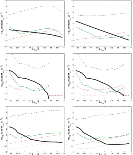
Fig. 1 shows the Bondi–Hoyle and the critical accretion rates for these six models and the two extreme values of the parameterη, representing the cases of both very efficient (η=1) and rather inef-ficient (η=0.1) accretion of angular momentum (see equation 9). One can see that the condition of radiation trapping is not very restrictive. Forη=1 it is satisfied forR<3×1011cm in models
RSG20 and RSG25, forR<3×1012cm in models RSG20He and
RSG25He, and much earlier forη=0.1.
On the contrary, the condition ˙MBH > M˙cn2 can be quite
re-strictive. In fact, it is never satisfied whenη=1. In this case, the circularization radius is always too far away from the NS and the neutrino cooling is not efficient enough. Forη=0.1, the results seem more promising as this condition is satisfied long way be-fore the NS merges with the core. For RSGs in the middle of the He-burning phase, this occurs almost at the same point where the ra-diation becomes trapped and a bit later for the pre-supernova RSGs. Thus, forη=0.1, the NS already begins to hyperaccrete inside the
2These models can be downloaded from the website http://homepages.
spa.umn.edu/∼alex/stellarevolution/.
envelope of the RSG primary. However, for such a small value ofη, the accretion disc becomes very compact and may even disappear, in which case the recycling efficiency is reduced.
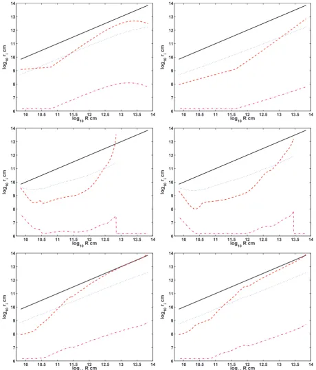
Fig. 2 shows all the characteristic radii of the in-spiral problem forη=0.1. One can see that for models RSG20 and RSG25, the disc accretion domain hasa>3×1010cm. For model RSG20He, this
domain includes the whole stellar envelope and for model RSG25He it splits into two zones. What is most important is that in all models the accretion begins to proceed with the Bondi–Hoyle rate while still in the disc regime.
Once the accretion disc is formed, the specific angular momentum of the gas settling on the NS surface is that of the last Keplerian orbit. In this case, the star will reach the rotational rate after accumulating
M≃ I jK ≃
0.18M0RNS2 ,6P−3 M⊙, (17)
whereI≃(2/5)MR2
NSis the final moment of inertia of the NS and
jKis the Keplerian angular momentum at the NS radius. Obviously,
the same mass is required to recycle the observed millisecond pul-sars in low-mass binaries and this allows us to conclude that the NS may well reach the gravitationally unstable rotation rate before collapsing into a BH.
When the accretion proceeds at the Bondi–Hoyle rate, the NS mass and orbit are related approximately as
aend
ainit =
Minit
Mend
σ
, (18)
whereσ = −Ma/˙ Ma˙ . Chevalier (1993) found that for a 10-M⊙ RSGσvaries slowly between 5 and 7. According to these results, the NS increases its mass by 0.2 M⊙after its orbital radius decreases by only a factor of few. This shows that the ‘window of opportunity’, where the disc accretion can proceed at the Bondi–Hoyle rate, does not have to be particularly wide. In order to obtain a more accurate estimate, one could integrate the evolution equation
˙
a a = −
4πG2Mρ
v3
M
M∗(1+M−2)3/2 +ζ CD ζ+3
ρ ρ
−1
,
(19) whereρis the average density of the primary insider=a,CD≈
6.5 is the drag coefficient (Shima et al. 1985) andζ=1+MN/M∗
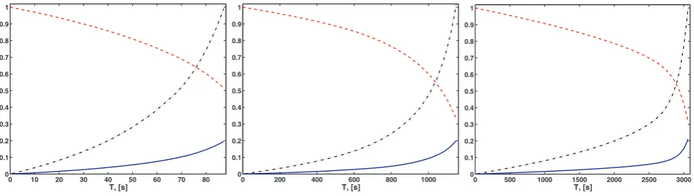
(Chevalier 1993). Figs 3 and 4 show the results of such integration for models RSG20, RSG25 and RSG25He, assuming that the hy-peraccretion regime begins near the stellar surface and ata=3× 1010cm, respectively. One can see that in all these cases the
gravi-tationally unstable rotation rate is reached whenadecreases by less than a factor of 5, in good agreement with the original estimate.
Forη=1, the mass accretion rate is low and the NS cannot spin up significantly inside the CE. What occurs in this case depends on the details of CE evolution. The CE can either be ejected leaving behind a close NS–WR binary or survive, leading to a merger of the NS and the RSG core (Taam & Sandquist 2000). The configuration after the merger is similar to that of the Thorne-Zydkow object (Thorne & Zytkow 1977; Barkov, Bisnovatyi-Kogan & Lamzin 2001). The common view is that such objects cannot exist because the effective neutrino cooling leads to hyperaccretion and prompt collapse of the NS into a BH. This conclusion is based on the spherically symmetric model, where the circularization radius is zero and the flow stagnation surface coincides with the surface of the NS. However, during the in-spiral the orbital angular momentum of the NS is converted into the spin of the primary. Thus, one would expect the core to be tidally disrupted and form a massive accretion
at University of Leeds on April 1, 2016
http://mnras.oxfordjournals.org/
Figure 1. Accretion rate as a function of the position inside the RSG primary for six different models: RSG2 (left-hand top panel), RSG3 (right-hand top panel), RSG20He (left-hand middle panel), RSG25He (right-hand middle panel), RSG20 (left-hand bottom panel) and RSG25 (right-hand bottom panel). The Bondi–Hoyle rate, ˙MB–H, is shown by the thick solid lines, the critical value ˙Mcn1is shown by the dotted (η=0.1) and dashed (η=1) lines, and the critical
value ˙Mcn2is shown by the thin solid (η=0.1) and dot–dashed (η=1) lines.
disc around the NS. As a result, the cooling rate will be lower compared with that found in the spherically symmetric case. It is not obvious for how long this configuration may exist. However, this again opens the possibility of the recycling of the NS up to the gravitationally unstable rotation rate and magnetically driven stellar explosion.
In the case of core collapse, even the magnetic field of magne-tar strength cannot prevent accretion and fails to drive the stellar
explosion (Komissarov & Barkov 2007). The magnetosphere be-comes locked under the pile of accreting matter and a separated mechanism, for example, the standard neutrino-driven explosion, is required to release it. However, the density around the Fe core of pre-supernovae is very high, leading to very high accretion rates. In our case, the accretion rates are expected to be significantly lower. In the next section, we explore if they are low enough to allow purely magnetically driven explosions.
at University of Leeds on April 1, 2016
http://mnras.oxfordjournals.org/
Figure 2.The characteristic radii of the in-spiral problem as functions of the position inside the RSG primary for the same models as in Fig. 1 andη=0.1. The orbital radius is shown by the solid line, the sonic point,Racc, is shown by the dotted line, the accretion shock radius is shown by the dashed line and the
circularization radius,Rc, is shown by the dot–dashed line.
3 M AG N E T I C E X P L O S I O N
3.1 Magnetic field generation
The main route to the formation of ‘magnetars’ is believed to be the core collapse of rapidly rotating stars. During the collapse, the proto-NS naturally develops strong differential rotation, with the
angular velocity decreasing outwards. This allows the generation of super-strong magnetic field via the α– dynamo (Duncan & Thompson 1992; Thompson & Duncan 1993) or magnetorotational instability (Burrows et al. 2007).
In our case, the conditions are rather different. The NS is already fully developed, with a solid crust, when it enters the envelope of its companion. The typical NS crust has the thicknessh≈105cm
at University of Leeds on April 1, 2016
http://mnras.oxfordjournals.org/
Figure 3. Evolution of the NS in the case when the Bondi–Hoyle regime begins at the surface of the RSG primary for models RSG25He (left-hand panel), RSG20 (middle panel) and RSG25 (right-hand panel). The lines show the accreted mass normalized to M⊙(solid line), the angular momentum of the NS normalized to the critical valuejc=Ic, wherec=760 Hz (dot–dashed line), and the orbital radius normalized to its initial value (dashed line).
Figure 4. The same as in Fig. 3, but for the case when the Bondi–Hoyle regime starts ata=3×1010cm.
and the density at the bottom ρ ∼1014g cm−3 (see e.g. Gnedin,
Yakovlev & Potekhin 2001; Lattimer & Prakash 2007). The NS may have already been spinned up via the accretion from the stellar wind, but its rotation rate may still be well below the critical for the development of the gravitational wave instability. In any case, the accreted gas of the companion’s envelope forms a very rapidly rotating layer above the crust. As long as the crust exists, this layer and the NS core are basically decoupled and interact mainly gravitationally. A strong tangential discontinuity exists at the outer boundary of the crust (Inogamov & Sunyaev 1999, 2010).
As the mass of the outer layer increases, the crust pressure goes up. Because of the degeneracy of the crust matter, its pressure depends mainly on its density, and only weakly on the temperature. When the density reaches the critical valueρcr∼1014g cm−3, the
crust begins to melt down (Brown 2000), and the barrier separating the NS core and its outer rotating layer disappears. If we ignore the centrifugal force, then this occurs when the NS accumulates mass comparable to the crust mass, ∼0.05 M⊙. The centrifugal force significantly reduces the effective gravitation acceleration and the above estimate for the layer mass is only a lower limit. Assuming
vφ≈vK∼1010cm s−1, the rotational energy of the layer at the time
of melting may well reach∼1052erg. Once the crust has melted,
the core and the layer can begin to interact hydromagnetically, with up toE∼1052erg of energy in differential rotation to be utilized.
One possibility is viscous heating and neutrino emission. We can estimate the neutrino luminosity as Lν ≈ E/td, where td is
the neutrino diffusion time. Following the analysis of Lattimer & Prakash (2007) and Barkov (2008), this time can be estimated as
td∼
hτν
c , (20)
where τν = hρν/mp is the optical depth of the hot envelope
for the neutrino emission. Assuming equilibrium with the elec-tron fractionYe=0.05, the mean neutrino cross-section is about
ν ≈σνǫνkTe/m2ec4, whereσν=1.7×10−44cm2(Bahcall 1964)
andǫν ≈3.15kTeis the mean energy of the neutrino (Thompson,
Burrows & Meyer 2001). The temperature can be estimated as
Te≈
E
4πarhR2
NS
1/4
≈1012
E521/4h− 1/4
5 R−
1/2 NS,6K,
wherear=7.564×10⁻¹⁵erg cm−3K−4is the radiation constant.
The corresponding diffusion time is quite short,
td∼
0.1h35/2ρ14E152/2
RNS,6
s.
Another process is the development of the Kelvin–Helmholtz instability, the production of the turbulence and amplification of magnetic field. For the Kelvin–Helmholtz instability to develop, the Richardson numberJhas to be less than 1/4 (Chandrasekhar 1961). In our case
J≈ gh v2
φ ≈
0.2RNS,6h5, (21)
at University of Leeds on April 1, 2016
http://mnras.oxfordjournals.org/
[image:8.595.46.545.256.397.2]whereg ≈ GMNS/RNS2 is the gravitational acceleration and we
useMNS =1.5 M⊙. Thus, the instability condition is marginally
satisfied. Once the turbulence has developed, the magnetic field amplification is expected to proceed as discussed in Duncan & Thompson (1992). The e-folding time is given by the eddy turnover time, which one would expect to be below the rotation period of the outer layer. Thus, strong magnetic field can be generated on the time below the viscous and the neutrino diffusion time-scale.3This conclusion is supported by the recent numerical
sim-ulations of similar problems, which show that the time as short as 0.03 s can be sufficient to generate dynamically strong magnetic field (Obergaulinger et al. 2009; Rezzolla et al. 2011). The strong toroidal magnetic field can suppress the instability ifρv2< B2/4π
(Chandrasekhar 1961) or ifB>3×10¹⁷G. This is likely to
de-termine the saturation strength of magnetic field. Such a strong magnetic field is also buoyant (Spruit 1999) and will emerge from under the NS surface into the surrounding accretion flow.
Another possibility of generating super-strong magnetic field in the recycled NS was proposed by Spruit (1999) with an application to X-ray binaries. In this model, the NS spins up to the critical rotation rate where it becomes unstable to exciting r modes and gravitational radiation (Levin 1999; Spruit 1999). This may lead to effective braking of the outer layers of the NS and developing strong differential rotation. Recent studies, however, suggest that non-linear coupling with other modes leads to the saturation of the r mode at a much lower amplitude (Arras et al. 2003; Brink et al. 2005; Bondarescu et al. 2007), though the mass accretion rates assumed in these studies are much lower than those encountered in CEs.
3.2 Criteria for explosions
Depending on the mass accretion rate, this may just modify the properties of the accretion flow near the star, the ‘accretor’ regime, or drive an outflow (e.g. Illarionov & Sunyaev 1975). In the latter case, two different regimes are normally discussed in the litera-ture, the ‘propeller’ regime and the ‘ejector’ regime. In the ejector regime, the magnetosphere expands beyond the light cylinder and develops a pulsar wind. In the propeller regime, the magnetosphere remains confined to the light cylinder. If the magnetic axis is not aligned with the rotational axis, then the magnetosphere may act in a similar fashion to an aircraft propeller, driving shock waves into the surrounding gas, heating it and spinning it up. If the en-ergy supplied by the propeller is efficiently radiated away, this may lead to a quasi-static configuration (e.g. Mineshige, Rees & Fabian 1991). If not, the most likely outcome is an outflow, followed by the expansion of the magnetosphere, and the transition to the ejector regime.
This classification is applied both in the case of quasi-spherical accretion and in the case of disc accretion. In the disc case, the external gas above and below the disc is usually not considered as important dynamical element. However, in our case, this is not true because the accretion disc is rather compact and feeds from a more or less spherical component of the accretion flow. If the expanding magnetosphere removes this component, the disc will no longer be supplied with mass and quickly disappear, no matter what its regime is. For this reason, we will not consider the complicated
3The viscous dissipation time-scale is very long t
vis ≈ 108R23NS/,46T92s
(Shapiro 2000).
interaction between the magnetosphere and the disc,4but will focus
on the interaction with the low angular momentum flow of the polar regions which accretes directly on to the NS avoiding the disc. In order to simplify the problem, we will treat this flow as spherically symmetric, keeping in mind that its mass accretion rate is only a fraction of the Bondi–Hoyle rate.
The extent of the magnetosphere is often estimated by the balance between the magnetic pressure and the ram pressure of accreting flow. This is fine when the accretion shock is close to the NS. If not, the thermal pressure at the magnetospheric radius can be signifi-cantly higher compared both to the actual ram pressure at the shock and to the ram pressure that would be found at the magnetospheric radius if the free-fall flow could continue down to this radius. In this case, the initial radius of the emerging magnetosphere is rather determined by the balance of the magnetic pressure and the thermal pressure of the quasi-hydrostatic ‘settling’ flow downstream of the accretion shock (Mineshige et al. 1991).
Assuming that the accretion flow in the polar region is approx-imately spherical, we can describe it using the analytical model developed by Houck & Chevalier (1991). Repeating their calcu-lations with the more accurate cooling function, adopted later in Chevalier (1996),
˙
ǫn=1025
kT
MeV
9
erg cm−3s−1 (22)
(Dicus 1972; Brown & Weingartner 1994) and using the adiabatic indexγ=4/3, we find the accretion shock radius
Rsh≃8.2×10⁸f1RNS40/,276M− 1/27
0 M˙−
10/27
0 cm, (23)
where
f1=
RNS
Rg
1−2Rg
RNS
−1/2
−1
−64/27
(24)
andRg=GM/c2is the gravitational radius of the NS. (In the
calcu-lations, we assume the Schwarzschild space–time.) For reasonable masses and radii of NSs, 0.27<f1<0.62. In particularf1=0.54
forM=M⊙andRNS=10 km. Downstream of the shock we have
an adiabatic subsonic flow with the mass density
ρ=ρsh
R Rsh
−3
, (25)
where
ρsh=
7 4π
˙
M
(GM)1/2R3/2 sh
(26)
is the mass density at the shock, the pressure
p= 6
7pram(Rsh)
R Rsh
−4
, (27)
where
pram(Rsh)=
˙
M√GM
4πR5/2
sh
(28)
is the ram pressure of the free-falling flow at the shock, the temper-ature
T =
12 11ap
1/4
, (29)
4An interested reader may find out more about the disc–magnetosphere
interaction from Ustyugova et al. (2006) and references therein.
at University of Leeds on April 1, 2016
http://mnras.oxfordjournals.org/
whereais the radiation constant, and the radial component of 4-velocity
u= − M˙
4πρR2
. (30)
Assuming that the magnetosphere expands until its magnetic pressure equals the gas pressure,5we find the radius of the dipolar
magnetosphere with the surface strengthBNSto be
Rm=5×10⁶f− 3/4
1 R
17/9 NS,6M−
2/9
0 M˙−
2/9
0 BNS,15cm. (31)
For this to be above the NS radius, the mass accretion rate should not exceed
˙
Mcr≃1.3×10³f1−27/8B 9/2 NS,15R
4 NS,6M−
1
0 M⊙yr−
1. (32)
The traditional criterion for the propeller regime is that the mag-netospheric radius is below the light cylinder radius
RLC=
cP
2π ≃4.8×10
6
P−3cm (33)
and above the corotation radius
Rcor=
GM 2
1/3
≃1.5×10⁶P−2/33M 1/3
0 RNS,6cm, (34)
at which the magnetosphere rotates with the local Keplerian veloc-ity.
The ejector regime is realized whenRm >Rc. In terms of the
mass accretion rate, the propeller regime criterion can be written as ˙
Mej<M <˙ M˙pr
and the ejector regime criterion as ˙
M <M˙ej,
where ˙
Mpr≃2×10²f− 27/8
1 M−
5/2
0 R
17/2 NS,6B
9/2 NS,15P−
3 −3M⊙yr−
1
(35)
and
˙
Mej≃1.1f− 27/8
1 M−
1
0 R
17/2 NS,6B
9/2 NS,15P−
9/2 −3 M⊙yr−
1
. (36)
The latter is much stronger and even if only a fraction of the total mass accretion rate is shared by the quasi-spherical component, it could be satisfied only during the early phase of the in-spiral (see Fig. 1). More likely, the emerged magnetosphere will operate in the propeller regime.
The sound speed in the Houck & Chevalier (1991) solution de-pends only of the NS mass and the distance from the NS,
cs≃6.2×10⁹M 1/2
0 R−
1/2
6 cm s−
1
. (37)
The linear rotational velocity of the magnetosphere,
vrot≃4.8×10⁹P−−31R6cm s−1, (38)
is generally higher and thus we have the so-called supersonic pro-peller. The power generated by such a propeller is roughly
Lpr≃
4π
3 pmR
2 m
(Rm)2
cs
≃1.3×1050f9/8
1 B
1/2 NS,15P−
2 −3M˙
1/3
0 M
1/6
0 erg s−1 (39)
5As a result of its oscillations, the NS can become quite hot and fill the
mag-netosphere with substantial amount of plasma. In this case, the centrifugal force will need to be included in the force balance, yielding an even higher value forRm.
(Mineshige et al. 1991), exceeding by several orders of magnitude the accretion power
Lacc=
GMM˙ RNS ≃
8×1045M0R−NS1,6M˙0erg s−1. (40)
This suggests that the magnetosphere easily blows away the accret-ing matter and expands beyond the light cylinder, thus creataccret-ing the conditions for a proper pulsar wind from the NS.
One may argue that the accretion flow could re-adjust to the new conditions, with the accretion shock moving farther out, the temper-ature at the magnetospheric radius rising and the enhanced neutrino cooling compensating for the propeller heating,Ln=Lpr. (A similar
problem has been analysed by Mineshige et al. 1991.) Given the strong dependence of the neutrino emissivity on the temperature, the cooling is expected to be significant only in the close vicinity of the magnetosphere. In the non-magnetic case, most of the cool-ing occurs in the volume comparable to the NS volume (Houck & Chevalier 1991). This suggests that in our case the cooling volume will be approximately the same as the volume of the magnetosphere. Then the energy balance can be written as
4π
3 R
3
mǫ˙n(T)=Lpr, (41)
where ˙ǫn(T) is given by equation (22). Solving this equation forRm,
simultaneously with the pressure balance
p(Rm)=
1 8πB
2 0 Rm RNS −6 , (42)
wherep(R) is given by equation (27), we find that
Rm
RNS ≃
0.6BNS5/18,15R−NS1,/66M 1/18
0 P
2/9
−3, (43)
independently of the mass accretion rate. Since in this solutionRm<
RNS, we conclude that the accretion flow cannot re-adjust itself and
will be terminated by the emerged magnetosphere. In the case of cold NSs, the pulsar wind power
Lw≃
μ24
c3
1+sin2θ m
≃6×1049B2 NS,15R
6 NS,6P−
4 −3 erg s−
1,
(44) whereμ=B0R2NSis the star magnetic moment andθmis the angle
between the magnetic moment and the rotational axis of the NS (Spitkovsky 2006). For a hot NS, the mass loading of the wind can be substantial, leading to even higher luminosity (Bucciantini et al. 2006; Metzger, Thompson & Quataert 2007). The energy released in the magnetically driven explosion is the rotational energy of the NS
Erot=
1 2I
2
≃1.6×1052M 0RNS2 ,6P
2
−3erg, (45)
whereI≃(2/5)MNSR2NSis the NS moment of inertia.
Inside the RSG core, the accretion rate is expected to be much higher. For example, in model RSG20He, the core densityρ≃8.6× 10²g cm−3and the pressurep
≃1.3×10¹⁹g cm2s−2, yielding the
Bondi accretion rate
˙
MB≃π(GM)
2ρ
c3 s
≃4.3×10⁵M
⊙yr−1. (46)
For such a high accretion rate, the propeller regime requires the magnetic field to be well in excess of 1015G, similar to what is
required in the magnetar models of GRBs. Whether such a strong dipolar magnetic field can be generated is not clear at present, as the observations of known magnetars suggest lower values. However, this could be a result of the short decay time expected for such a strong field (Heyl & Kulkarni 1998).
at University of Leeds on April 1, 2016
http://mnras.oxfordjournals.org/
4 S U P E R N OVA P R O P E RT I E S
4.1 The plateau
Since the NS has to reach the maximum allowed rotation rate before it explodes, the model predicts the explosion energy around 1052erg,
putting it on the level of hypernovae. The corresponding ejecta speed will be very high
vej=109M− 1/2
ej,1 cm s−1, (47)
whereMej,1is the ejected mass.
Since the progenitor is a RSG, the supernova spectra will show hydrogen lines and would be classified as Type II. As the NS spirals through the weakly bound outer envelope of its RSG companion, it drives an outflow with the speed about the local escape speed and the mass-loss rate about M⊙yr−1 (Taam & Sandquist 2000).
The total in-spiral time is about few initial orbital periods. For a RSG with mass 20 M⊙and thew radiusR=1014cm, this yields
vesc=5×106cm s−1 andtins ∼few×108s. Thus, we expect a
hydrogen-rich circumstellar shell of few solar masses to exist at a distance of∼1015cm at the time of the supernova explosion. The
presence of such a shell will delay the transition to the adiabatic expansion phase and increase the supernova brightness similar to how this occurs in Type IIn supernovae (Chugai et al. 2004; Smith et al. 2007, 2008; Woosley, Blinnikov & Heger 2007).
Following Kasen & Bildsten (2010), the supernova luminosity during the phase of adiabatic expansion can be estimated as
L≃ Erotte t2
d
, (48)
wherete=R0/vejis the expansion time-scale andR0is the progenitor
radius, and
td=
3
4π
Mejk
cvej
1/2
(49)
is the radiative diffusion time-scale andkis the opacity. (In the estimates below, we usek=0.4 cm2g−1, the value for Thomson
scattering in the fully ionized plasma.) It is assumed that the initial magnetar spin-down time-scale is smaller compared tote, which
is certainly satisfied in our case, given the large required magnetic field, 1015–1016G. For the characteristic parameters of the model,
we have
te≃105R0,14vej−,19s, td≃8×10⁶M 1/2 ej,1v−
1/2
ej,9 s, (50)
and
L≃1.6×1043R0,14Mej,1erg s−1. (51)
This high luminosity will be sustained for up tot∼td, after which
the trapped radiation, generated by the blast wave when it was cross-ing the star, escapes and the luminosity drops. It most normal Type II supernovae, the luminosity after this point is sustained via the ra-dioactive decay of isotopes, mainly56Ni, produced by the supernova
shock in the high-density environment around the collapsed core. However, in our model, the stellar structure is significantly different from that of normal pre-supernovae.
4.2 56Ni production
If the explosion occurs after the NS is settled into the centre of RSG20He, then the core density is onlyρc≃8×10²g cm−3and
its temperatureTc≃1.9×10⁸K, andRA =GM/c2s is the Bondi
accretion radius.
As the magnetically driven explosion develops, a shock wave propagates through the body of the RSG. Where the post-shock temperature exceedsTNi≃109K,56Ni is produced in abundance
(Woosley et al. 2002). In order to capture the shock dynamics, we need to know the structure of the accretion flow on to the NS, which has been established before the explosion. This flow is rather com-plicated because of its rotation and without computer simulations we can only make very rough estimates.
First, consider the polar region where the flow is more of less spherically symmetric. Equation (13) shows that the accretion shock is quite close to the NS, particularly when it is near the RSG core, and hence most of the flow can be described using the free-fall model. The ram pressure of the accretion flow in this model is given by
ρv2 ff=
˙
M√2GM
4π R
−5/2, (52)
wherevff=(2GM/R)1/2is the free-fall speed. Close to the NS, the
speed of the explosion shock,vsh, is much less compared tovffand
can be found from the pressure balance equation 2
γ+1ρv
2 ff=
E
4πR3, (53)
whereRis the shock radius andE=Lwtis the energy injected by
the magnetar. This yields
t= 2 ˙M
√ 2GM
(γ+1)Lw
R1/2 (54)
and thus the shock speed increases with the distance. This approxi-mation breaks down at the radius
Rt=
2 ˙MGM
(γ+1)Lw
, (55)
wherevsh=vff. The gas temperature exceedsTNiinside the radius
RNidetermined by the equation
2
γ+1ρv
2 ff=
a
3T
4
Ni, (56)
and the total mass of the produced56Ni can be estimated as
MNi=Mt˙ Ni, (57)
wheretNiis the time required for the shock to reachRNiaccording
to equation (54). From equations (55–57), we find that
Rt=108M˙6L−w1,50cm, (58)
RNi=7.8×10⁷M˙ 2/5
6 cm, (59)
MNi=0.003 ˙M611/5L− 1
w,50M⊙. (60)
Thus, only a relatively small amount of56Ni can be produced even
for the highest mass accretion rates allowed in this model. In the equatorial plane, the accretion shock can be pushed all the way towardsRacc(see Section 2). Downstream of the shock, the
flow is highly subsonic with
ρ=ρ0
R R0
−3
. (61)
The highest density is achieved when the accretion shock is in-finitely weak and this law is applied up to the sonic pointRacc. In
this case, we can putR0=Raccandρ0=ρ∗, the mass density of
the RSG. The equation for shock speed is now 2
γ+1ρv
2
= E
4πR3, (62)
at University of Leeds on April 1, 2016
http://mnras.oxfordjournals.org/
which yields the shock radius
R= 2
3
(γ+1)Lw
8πρ
∗R3acc
1/2
t1/2. (63)
RNiis now determined by the equation
2
γ+1ρv
2
= aT
4 Ni
3 , (64)
where the mass of the produced56Ni is still given by equation (57).
Combining equations (63) and (64), we find
MNi∝MR˙ 9acc/7ρ 3/7
∗ L
1/7
w . (65)
The highest values forMNiare obtained inside the RSG core. For
model RSG20He, whereRacc∼5×109cm, ˙M∼106M⊙yr−1(see
Figs 1 and 2) andρ∗∼5×10²g cm−3, we findM
Ni≃0.02 M⊙.
Although significantly higher, this is still small compared to the mass deduced from the observations of most supernovae.
If the density behind the shock wave is lower than 106g cm−3,
which corresponds to ˙M <106M
⊙yr−1, then the photon dissoci-ation of Ni56becomes important as well (Magkotsios et al. 2010).
Thus, our estimation gives only an upper limit to the amount of the produced Ni56.
Another potential source of56Ni is the wind from the accretion
disc itself, like in the collapsar model of a GRB. Without a robust disc model, it is difficult to figure out how effective this mecha-nism is. For example, in the numerical simulations of MacFadyen & Woosley (1999), the outcome was dependent on the rate of the introduced ‘viscous’ dissipation. In any case, the much lower ac-cretion rates encountered in our model suggest that the amount of
56Ni will be lower too. Thus, we conclude that our model predicts
significant deficit of56Ni.
4.3 The long-term effects of the magnetar wind
It has been suggested recently that the long-term activity of mag-netars born during the core collapse can power the supernova light curves, mimicking the effect of radioactive decay (Kasen & Bildsten 2010; Woosley 2010). In these studies, it was assumed that the rotational energy of the magnetar, released at the rate∝t−2, is
converted into heat at the base of the supernova ejecta. One mech-anism of such heating is purely hydrodynamical, via the forward shock wave involved in the collision of the fast magnetar wind with the slower supernova ejecta. In our case, however, this shock is the supernova shock and it is not present since the break-out. The other mechanism, heating by the radiation produced at the termination shock of the magnetar wind, remains in force and here we explore its efficiency.
Combining equations (44) and (45), it is easy to obtain the well-known law of the asymptotic spin-down of magnetic rotators
=
I c3
2μ2t
1/2
≃40BNS−1,15t− 1/2
7 s−
1
(66)
and
Lw=
1 4
I2c3
μ2t2 ≃10 41
BNS−2,15t−2 7 erg s−
1
. (67)
(In this section, we useRNS=106cm andMNS=1.5 M⊙.) The last
equation shows that unlessB<1015G the supernova luminosity will
drop dramatically after the plateau phase. Such evolution has been observed in some supernovae, for example, SN 1994W (Tsvetkov 1995; Sollerman, Cumming & Lundqvist 1998).
In order to see how exactly this energy can be used to heat the supernova ejecta, we can appeal to the observed properties of pulsar
wind nebulae. For example, the study of the Crab nebula by Kennel & Coroniti (1984) indicates that immediately behind the termination shock most of the energy is in the form of ultrarelativistic electrons and only a fraction of it is in the magnetic field and there is no good reason to expect this to be different for magnetar winds. However, the magnetic field of a 1-yr-old magnetar wind nebula (MWN) is expected to be very strong, making the synchrotron cooling time very short.
One can estimate the magnetic field strength via the pressure balance at the termination shock
Lw
4πR2
wc
= B
2
8π, (68)
whereRw is the radius of the termination shock. Assuming that
Rw≃vejt, this yields
B≃0.3t7−2B− 1 NS,15v−
1
ej,9G. (69)
The lowest energy electrons accelerated at the termination shock of the Crab nebula have the Lorentz factorγ ∼ 106 (Kennel &
Coroniti 1984). In the magnetic field of the MWN, they produce synchrotron photons with energy
Eν ≃100B−0,115v− 3/2 ej,9 t−
2
7 keV (70)
and their synchrotron cooling time
tsyn≃104t74B 2 NS,15v
2
ej,9s (71)
is shorter compared to the dynamical time-scale for few years after the explosion.
The observations of the Crab nebula also show that the electrons are accelerated up to the radiation reaction limit (de Jager et al. 1996; Komissarov & Lyutikov 2011). Assuming that the same is true in our case, we expect the synchrotron spectrum to continue up toEmax
ν,syn≈100 MeV and the highest energy of the electrons to be
Eemax≃100t7B 1/2 NS,15v
1/2
ej,9TeV. (72)
These electrons also cool via the IC scattering on the soft pho-tons produced by the supernova shell. The ratio of the IC to the synchrotron energy lossesξ = usoft/uB, whereusoft is the energy
density of the soft radiation anduB =B2/8πis the magnetic
en-ergy density. During the plateau phase
usoft≃
Lsoft
4πR2
phc
, (73)
whereRphis the radius of the photosphere. Combining this result
with equation (68), we find
ξ≃ Lsoft Lw Rw Rph 2 . (74)
As we have seen,Lsoft can be much higher than Lw but, on the
other hand, Rw can be much lower than Rph. Thus, it is hard to
tell whether the IC emission can compete with the synchrotron one without detailed numerical simulations.6 After the plateau phase,
usoftdrops dramatically and we expect the synchrotron losses to be
dominant.
6Should the IC losses dominate,Emax
e andEν,maxsynare to be reduced by the
factorsξ1/2andξ, respectively.
at University of Leeds on April 1, 2016
http://mnras.oxfordjournals.org/
For photons with energyEν≤mec2∼0.5 MeV, the main source
of opacity is the Compton scattering in the Thomson regime. The corresponding optical depth is
τT≃σTMej/4πmp(t vej)2≃6Mej,1t7−2v− 2
ej,9, (75)
whereσT is the Thomson cross-section. Thus, the shell becomes
transparent in about 1 yr after the explosion. The typical energy of photons from radioactive decays is around 1 MeV and hence the ejecta opacity to these photons is similar. As a result, the synchrotron photons and the photons from radioactive decays are utilized with similar efficiency.
WhenEν≫mec2the scattering is in the Klein–Nishina regime
and the cross-section is smaller,σKN≈3σTmec2/8Eν(Lang 1980).
For 100-MeV synchrotron photons, this yields
τKN≃10−2Mej,1t7−2v− 2
ej,9 (76)
and these photons begin to escape already after 10 d or so. However, provided the spectrum of the shock-accelerated electrons is a power lawN(E)∝E−pwithp>2, which is expected to be the case, the contribution of such highly energetic photons to the energy transport is lower.
The IC photons with energyEν > (2mec2)2/Eν,soft ≃ 1.2 TeV
will also interact with the soft supernova photons via the two-photon pair-production reaction (here we usedEν,soft=1 eV). The
corresponding opacity can be estimated as
τγ γ ≃
σT
5
Lsoft
4π(vejt)cEsoft ≃
2Lsoft,41vej−,19t− 1
7 . (77)
Thus, we expect the ejecta to become transparent to the IC emission soon after the end of the plateau phase.
The above calculations show that during the plateau phase the high-energy emission from the termination shock of the magnetar wind is deposited in the ejected envelope. However, this additional heating has little effect on the supernova luminosity. Indeed, the increase in the luminosity due to this heating can be estimated as
L≃ Erot(t)t t2
d
≃ Lw(t)t
2
t2 d
=Lw(td)≪L. (78)
Fort>td the energy deposition rate does no longer scale ast−2
(cf. Woosley 2010) as the ejecta becomes transparent to the high-energy emission. For example, if the synchrotron emission is the main channel of heating, then the rate scales asLwτ∝t−4whenτ <
1, and the rate due to IC emission is likely to decline even faster. Out of the well-studied supernovae known to the authors, none fits the above description. The closest example is SN 1994W (Cortini et al. 1994; Sollerman et al. 1998). This is one of the brightest Type II supernovae with the peak luminosity∼1043erg s−1. After around
120 d its luminosity drops dramatically down to∼1041erg s−1. The
tail of its light curve is very steep showing very small mass of the ejected56Ni (Sollerman et al. 1998). In fact the data can be
approximated byL∝t−4.6. All these properties agree nicely with
our expectations. On the negative side, the spectral data indicate the lower ejecta speed and the presence of a very slow component withv∼1000 km s−1. This supernova is classified as Type IIn and
seems to be explained very well in the model involving a collision between the SN ejecta and a massive circumstellar shell ejected few years earlier in the giant stellar eruption (Chugai et al. 2004; Smith et al. 2007, 2008; Woosley et al. 2007).
The power of the escaped high-energy emission can be estimated asLγ ≃Lwe−τ. As usual in such cases, it will peak whenτ∼1,
which may occur within the first year after the explosion. For a source at the distanced=10d1Mpc, the corresponding total flux
will be
Fpeak≃3×10⁻¹²BNS−2,15t− 2 p,7d−
2 1 erg cm−
2
s−1, (79) wheretpis the time when the peak is reached. For the synchrotron
component, the spectral energy distribution is expected to peak aroundEν=100 keV (see equation 70).
4.4 Remnant
What is left behind after the explosion depends on where inside the RSG it occurs. As we have demonstrated, this strongly depends on the mean specific angular momentum of the gas captured via the Bondi–Hoyle mechanism. If it is as high as proposed in the early investigations (Illarionov & Sunyaev 1975; Shapiro & Lightman 1976), then the NS will accrete only at the Eddington rate until it settles into the core of its companion. What would happen after this is not clear. The current view is that the neutrino cooling will be sufficiently high for the accretion to proceed at the Bondi rate and that the NS collapses into a BH (Zel’dovich, Ivanova & Nadezhin 1972). However, this conclusion is based on spherically symmetric models. The high rotation rate developed in the core of the primary during the in-spiral means that instead of directly accreting on to the NS the core will form a torus, whose neutrino cooling may not be very effective, in which case such a configuration can be relatively long-lived. Moreover, the mass accretion will be accompanied by the efficient recycling of the NS, so one can still expect the NS to turn into a millisecond magnetar before its mass becomes high enough for gravitational collapse. Even if the magnetar-driven explosion fails in the dense environment of the core, and the NS eventually collapses into a BH, this will be a rapidly rotating BH accompanied by a massive accretion disc – the configuration characteristic of the collapsar model for a GRB. However, in contrast to the GRB progenitors, the envelope of the RSG star is not sufficiently compact for the relativistic jet to penetrate it during the typical lifetime of the GRB central engine. Instead, the jet energy will be deposited in the RSG envelope and most likely result in a supernova explosion, leaving behind a BH remnant. Interestingly, the mass of the pre-supernova could be below the limit for BH formation in the normal course of its evolution as a solitary star.
If the angular momentum is much lower, as suggested by Davies & Pringle (1980), then the explosion occurs when the NS is still inside the RSG envelope and then the remnant is likely to be a close binary consisting of a WR star and a magnetar.7In order to
show this, we first note that the pressure inside the core of the RSG at the He-burning phase is pc ∼ 1019erg cm−3 and much higher
at the pre-supernova phase (Woosley et al. 2002). This has to be compared with the pressure inside the high-entropy bubble, created by the magnetar,
pb≃
Lwt
4πR3
b
(80)
whereRb=vbtis the bubble radius,vbis its expansion speed and
tis the time since the explosion. We are interested in its value at the time when the bubble radius is comparable with the separation between the NS and the RSG core. TakingRp =1010Rb,10cm and
t=Rb/vb, we find that
pb≃1019Lw,49v−b,19R− 2
b,10erg cm−
3. (81)
7The 2D numerical simulations by Fryer et al. (1996) have indicated the
possibility of a neutrino-driven explosion during the CE phase, also leaving behind a close binary system.
at University of Leeds on April 1, 2016
http://mnras.oxfordjournals.org/