Sensitivity Analysis of an Advanced Gas-Cooled Reactor Control Rod Model

This is a repository copy of

Sensitivity Analysis of an Advanced Gas-Cooled Reactor

Control Rod Model

.

White Rose Research Online URL for this paper:

http://eprints.whiterose.ac.uk/81828/

Proceedings Paper:

Scott, M., Sims, N.D., Green, P.L. et al. (2 more authors) (2014) Sensitivity Analysis of an

Advanced Gas-Cooled Reactor Control Rod Model. In: Proceedings of ISMA 2014,

International Conference on Noise and Vibration Engineering. ISMA 2014, International

Conference on Noise and Vibration Engineering, 15-17 September 2014, Leuven,

Belgium. .

[email protected] https://eprints.whiterose.ac.uk/ Reuse

Unless indicated otherwise, fulltext items are protected by copyright with all rights reserved. The copyright exception in section 29 of the Copyright, Designs and Patents Act 1988 allows the making of a single copy solely for the purpose of non-commercial research or private study within the limits of fair dealing. The publisher or other rights-holder may allow further reproduction and re-use of this version - refer to the White Rose Research Online record for this item. Where records identify the publisher as the copyright holder, users can verify any specific terms of use on the publisher’s website.

Takedown

If you consider content in White Rose Research Online to be in breach of UK law, please notify us by

Sensitivity Analysis of an Advanced Gas-Cooled Reactor

Control Rod Model

M. Scott1

, P. L. Green1

, C. Grant-Wilson2

, M. Bateman2

, K. Worden1

, N. D. Sims1 1

Dynamics Research Group, Department of Mechanical Engineering, University of Sheffield, Mappin Street, Sheffield S1 3JD, UK

e-mail: [email protected]

2

EDF Energy, Barnett Way, Barnwood, Gloucester, GL4 3RS

Abstract

A model has been made of the primary shutdown system of an Advanced Gas-cooled Reactor nuclear power station. The aim of this paper is to explore the use of sensitivity analysis techniques on this model. The two motivations for performing sensitivity analysis are to quantify how much individual uncertain parameters are responsible for the model output uncertainty, and to make predictions about what could happen if one or several parameters were to change. Global sensitivity analysis techniques were used based on Gaussian process emulation; the software package GEM-SA was used to calculate the main effects, the main effect indexand thetotal sensitivity indexfor each parameter and these were compared to local sensitivity analysis results. The results suggest that the system performance is resistant to adverse changes in several parameters at once.

1

Introduction

The United Kingdom has seven Advanced Gas-cooled Reactor nuclear power stations (AGRs), which pro-vide around 20% of its electricity. The AGR design was developed in the 1970s and is unique to Britain. The primary shutdown mechanism is provided by the control rods which absorb the neutrons needed to sustain a chain reaction of uranium fissions in the reactor core. The control rods are continually raised and low-ered in order to maintain a critical reaction. A reactor typically has around 80 control rods, each with its own actuator. Should the reactor exceed its normal operating conditions, the control rods will be released by an electromagnetic clutch and insert into the core under gravity, shutting down the reactor. This system was designed experimentally and is regularly tested to ensure the rods will enter the core quickly enough to shutdown the reactor with a sufficient safety margin. Large amounts of collected data and modern modelling techniques give an opportunity to understand and monitor the primary shut down system performance at a more detailed level; this is beneficial for managing the plant commercially and for giving early warning of any potential performance issues. The objective of this paper is to develop a mathematical model of the system and explore the use of probabilistic sensitivity analysis techniques on this model.

It is relatively straightforward to assess the local sensitivity of a model to its parameters, by partially dif-ferentiating the model output with respect to different parameters. However this method is not particularly informative because it fails to take into account nonlinear responses. A slightly more informative technique is to run the model for a range of parameter values, keeping the others constant. Both of these methods fail to take into account the fact that sensitivity to a parameter could vary as other parameters change. For a model with many parameters assessing the effects of all possible parameter combinations is challenging [1]. Global sensitivity analysis techniques investigate the entire range of the possible input space using statistical methods; these can be time consuming and still require careful interpretation.

Monte Carlo analysis can be used to sample from the probability distribution of model outputs, given a set of probability distributions of model inputs, these output distributions can be used to infer global sensi-tivity qualities [2, 3]. Whilst this is effective, it can be extremely computationally expensive, especially if there are many parameters of interest. A way of reducing the expense of global sensitivity analysis given a computationally expensive model is to use a surrogate model - a model of a model. This still requires many model runs but far fewer than Monte Carlo analysis. A technique based on Fourier amplitude sensitivity test-ing (FAST) provides an elegant way of estimattest-ing the contribution of input uncertainty to output uncertainty, however this method is limited to investigating the main effects of parameters and does not give information regarding interactions. [4, 5].

Choosing sensitivity analysis techniques requires a compromise between robustness, computational cost, ease of implementation and conceptual simplicity. Within the nuclear industry, robustness is generally pre-ferred at the expense of computational cheapness, to within reason [6]. In the current case, the purpose of the model and sensitivity measures is to assist in decision making and increase understanding of the system. It is desirable that the meaning of the measures used and the concepts behind them are sufficiently intuitive that someone with little knowledge of sensitivity analysis is able to confidently use them.

The technique chosen in this investigation is a Bayesian approach to surrogate modelling developed in [7], which will be introduced in more detail below. It was chosen as it is both computationally efficient and robust, and although the maths behind it is relatively complicated the basic principles are not difficult to understand.

2

The model

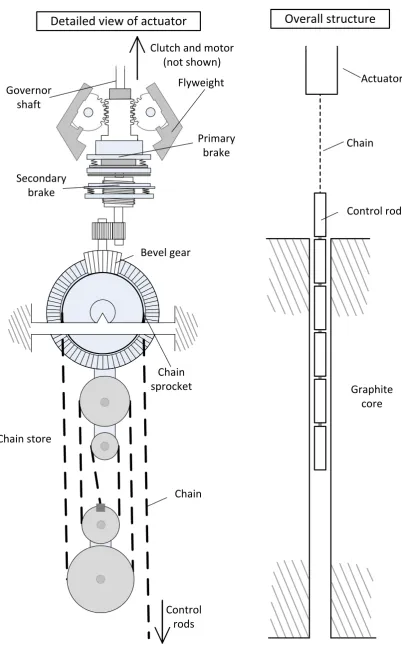
A schematic of the system of interest is shown in Figure 1 and a more detailed sketch of the brake system is given in Figure 2. The governor shaft is connected to the motor by an electromagnetic clutch (not shown). If power to the clutch is lost then the governor shaft will be released and the rods will insert into the core. A two-stage braking mechanism is attached to the governor shaft. The primary brake is driven by flyweights and is dependent on the rod velocity. The secondary brake is driven by a lead screw, which is connected to the bevel shaft by gears (not shown). Key assumptions made during the derivation of the model structure are:

• The effects of the chain friction, bearing friction, gear/sprocket efficiency and the friction between the side walls of the core and the rods are lumped together in a single, scaled friction parameterFf which acts as a constant force resisting the rod motion.

• The coefficient of friction between the governor and the brake is a constant.

• The drag forces from the gas are directly proportional to the velocity of the rods and do not depend on the displacement.

Chain

Control rods

Graphite core

Chain store

Chain Bevel gear

Chain sprocket Governor

shaft

Control rods Secondary

brake

Primary brake

Flyweight Actuator

Clutch and motor (not shown)

Overall structure

Detailed view of actuator

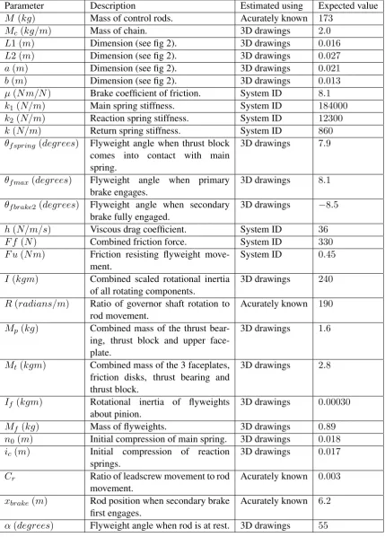
Rod at rest _{secondary brakes engaged}Rod moving, primary and Dimension a Dimension b Dimension L1 Angle Main spring Reaction spring Lead screw Primary brake friction disk Secondary brake friction disk Flyweight Flyweight centre of mass Pinion

Dimension L2

Angle +

Figure 2: The primary and secondary brake mechanisms.

The action of the brake is sufficiently complicated that there are 9 distinct stages of rod motion. Each stage is described by 2 simultaneous differential equations, one for the motion of the rods and one for the motion of the flyweights. The points at which the model transitions between stages are dictated by the position of the flyweights and the rods. The equations describing stage 6 of the rod’s motion are given as an example below.

The rod acceleration,x¨_{, is given by:}

¨

x₌ M g+Mcgx−hx˙ −Ff −(C1x˙ 2

−C8θ_f −C9)−(C10+C11θ_f +C12x)

M+Mcx+I

(1)

Where:

c=L1sin(α+θf)

d=L1cos(α+θ_f)

C8 =µRb(k+k1)

C9 =µR(M f gc/b+C_b−M_pg)

C10=µRk2(i_c+L2−x_ubrake−bθ_{f max})

C11=µRk2b

C12=µRk2Cr The acceleration of the flyweights is given by:

¨

θ_{f =} Cax˙ 2

−Mfgc−(kbθf−Mpg)b−Fusgn( ˙θf)−(k1bθ_f +C_b)b−(C5+C6θ_f +C7x) (If +Mtb2)

(2)

Where:

C5=k2b(i_c+L2−x_ubrake−bθf max)

C6=k2b 2

Parameter Description Estimated using Expected value

M (kg) Mass of control rods. Acurately known 173

Mc(kg/m) Mass of chain. 3D drawings 2.0

L1 (m) Dimension (see fig 2). 3D drawings 0.016

L2 (m) Dimension (see fig 2). 3D drawings 0.027

a(m) Dimension (see fig 2). 3D drawings 0.021

b(m) Dimension (see fig 2). 3D drawings 0.013

µ(N m/N) Brake coefficient of friction. System ID 8.1

k1(N/m) Main spring stiffness. System ID 184000

k2(N/m) Reaction spring stiffness. System ID 12300

k(N/m) Return spring stiffness. System ID 860

θf spring(degrees) Flyweight angle when thrust block comes into contact with main spring.

3D drawings 7.9

θf max(degrees) Flyweight angle when primary brake engages.

3D drawings 8.1

θf brake2(degrees) Flyweight angle when secondary brake fully engaged.

3D drawings −8.5

h(N/m/s) Viscous drag coefficient. System ID 36

F f (N) Combined friction force. System ID 330

F u(N m) Friction resisting flyweight move-ment.

System ID 0.45

I (kgm) Combined scaled rotational inertia of all rotating components.

3D drawings 240

R(radians/m) Ratio of governor shaft rotation to rod movement.

Acurately known 190

Mp(kg) Combined mass of the thrust bear-ing, thrust block and upper face-plate.

3D drawings 1.6

Mt(kgm) Combined mass of the 3 faceplates, friction disks, thrust bearing and thrust block.

3D drawings 2.8

If (kgm) Rotational inertia of flyweights about pinion.

3D drawings 0.00030

Mf (kg) Mass of flyweights. 3D drawings 0.89

n0(m) Initial compression of main spring. 3D drawings 0.018

ic(m) Initial compression of reaction springs.

3D drawings 0.017

Cr Ratio of leadscrew movement to rod movement.

Acurately known 0.003

xbrake(m) Rod position when secondary brake first engages.

Acurately known 6.2

α(degrees) Flyweight angle when rod is at rest. 3D drawings 55

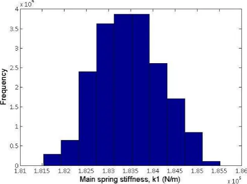
Figure 3: Histogram of k1 probability distribution.

The model relies on 28 parameters which represent physical attributes of the system e.g. spring stiffnesses, masses, coefficients of friction etc. These parameters are listed in Table 1. Some of the parameters (the gear ratios and the mass of the rods) are accurately known quantities. Many of the parameters were estimated using 3D models of the system which are fairly accurate, but their accuracy cannot be guaranteed. There were some parameters which are not possible to measure directly or estimate analytically with any accuracy. These were the friction terms, spring stiffnesses, and the viscous drag coefficient.

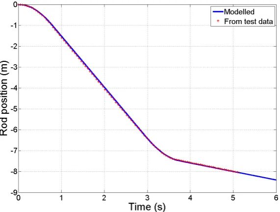
The system is tested regularly and time histories of the rod positions have been recorded. The possible values of the unknown parameters were estimated using Bayesian system identification, which combines prior knowledge of the parameters with measured data from the system to give probability distributions of parameter values. An example of this is given in Figure??, which shows the probability distribution for the stiffness of the primary brake main spring, k1. The data used was a single time history taken from the insertion test of a newly maintained system. A plot of this time history is given in Figure??alongside a plot of the modelled rod position (the model used the mean of the estimated parameter probability distributions for the unknown parameter values). Describing the details of Bayesian system identification is outside the scope of this paper, the techniques used here were developed in [8] and [9].

The sensitivity analysis methods used in this investigation require the model to give a single value output. The value chosen here is the distance the rod has inserted 4.5 seconds after it has been released, which was chosen as it is used as a key measure of how well the primary shutdown system is performing. The design specification is that the rods must have inserted at least 6.5m after 4.5 seconds to shutdown the reactor with a sufficient safety margin. It is desirable that the rods enter the core as quickly as possible, while not traveling fast enough to cause any damage.

3

Bayesian Sensitivity analysis

3.1 The Emulator

Figure 4: Plot of measured rod position and modelled rod position during an insertion test.

vectors as inputs to provide the training data for creating the emulator.

If it is assumed that the model is a smooth function of its inputs, then a response surface can be fitted to the training data using a least squares regression and the output can be estimated for any set of inputs. Early use of emulators in sensitivity analysis involved using the response surface to perform Monte Carlo analysis at a reduced cost [3]. In the current case the response surface is used to provide the mean of the multivariate Gaussian probability distribution which represents the prior belief in the value of the model output. The prior distribution is then conditioned on the training data to give a posterior distribution over functions, which can be used to infer many global sensitivity values, the ones of interest will be described below. This technique is described in detail in [7].

3.2 Main effects and interactions

The model output, y can be decomposed into main effects and interactions of its input parameters, x (x denotes the vector ofninput parameters{x1, ..., x_n})

y=E(Y) + n X

i=1

zi(xi) + X

i<j

zi,j(xi,j) X

i<j<k

zi,j,k(xi,j,k) +...+zi,j,k(x) (3)

where,

zi(xi) =E(Y|xi)−E(Y) (4)

zi,j(xi,j) =E(Y|xi, j)−zi(xi)−zj(xj)−E(Y) (5)

zi,j,k(xi,j,k) =E(Y|xi, j, k)−zi,j(xi,j)−zi,k(xi,k)−zj,k(xj,k)−zi(xi)−zj(xj)−zk(xk) (6)

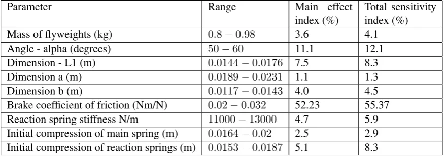
Parameter Range Main effect index (%)

Total sensitivity index (%) Mass of flyweights (kg) 0.8−0.98 3.6 4.1

Angle - alpha (degrees) 50−60 11.1 12.1

Dimension - L1 (m) 0.0144−0.0176 7.5 8.3 Dimension a (m) 0.0189−0.0231 1.1 1.3 Dimension b (m) 0.0117−0.0143 4.0 4.5 Brake coefficient of friction (Nm/N) 0.02−0.032 52.23 55.37 Reaction spring stiffness N/m 11000−13000 4.7 5.9 Initial compression of main spring (m) 0.0164−0.02 2.5 2.9 Initial compression of reaction springs (m) 0.0153−0.0187 5.1 8.3

Table 2: Main effect index and total sensitivity index values for most important parameters from the first run of sensitivity analysis.

The main effect of a parameter is the output of the model with the parameter held constant, averaged over all of the other parameters’ possible values. This can be plotted over the parameter’s possible range and gives a good visual representation of the model’s sensitivity to that parameter. A plot of the interactions shows the effect of varying two or more parameters simultaneously (in addition to their main effects) averaged over the rest of the parameter space.

3.3 Variance based measures

The variance of the main effect is known as themain effect index(MEI) and it can be written as,

MEIi= var{E(Y|Xi)} (7)

This is the expected amount that the uncertainty of the model output would be reduced if the true value ofxi was known.

The total sensitivity index (TSI) is the variance caused by a parameter and any interaction involving that parameter,

TSIi= var(Y)−var{E(Y|X₋i)} (8) It can also be thought of as the remaining variance if the true values of all of the parameters exceptxi are known (−irefers to the complement of the subseti).

For a more detailed description of these measures, and how they are inferred see [7] and [10].

4

Results and discussion

4.1 The first run of sensitivity analysis

The purpose of the first run of sensitivity analysis performed here is to investigate how the uncertainty in individual model parameters is responsible for the uncertainty of the model output. This can be used to decide which parameters are most important when developing the model, as well as giving insight into how the system behaves. There are 25 parameters which were investigated here out of 28 in total. The mass of the rods, the gear ratios and the gravitational constant are all known accurately and are not going to change. 18 of the parameters were measured from 3D drawings of the system which are thought to be reasonably ac-curate. For these parameters a range of±10%either side of the parameter’s expected value was used, which is likely to be far in excess of the actual inaccuracy. Probability distributions for the other 7 parameters were estimated using Bayesian system identification, however these distributions were estimated assuming that the other parameter values were accurate, so the ranges used have been doubled.

At this point it is worth noting the difference between subjective and objective uncertainty in parameter values. Subjective uncertainty results from a lack of accurate knowledge of the system, e.g. a dimension which is not accurately known. Objective uncertainty results from the fact that some elements in the system behave in a stochastic way, for instance, brake pad friction coefficients have been shown to vary unpre-dictably [11].

The MEIs and TSIs of the parameters which were responsible for more than 1% of the output variance are shown in Table 2. It can be seen that more than half of the output variance arises from the brake friction termµ. It is also clear from the table that the vast majority of the variance arises from the main effects of parameters, since the values of the MEIs are close to the values of the TSIs. The sum of the MEIs is 95%, so interactions account for only around 5% of the output variance.

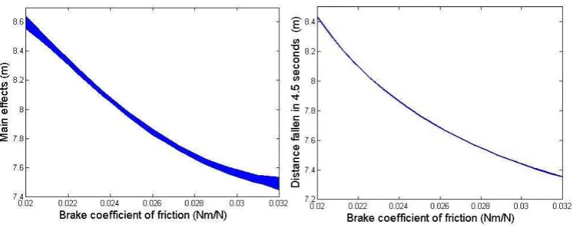
Plots of the main effects for selected parameters are shown in Figure 5 to 8. Alongside these are plots of the model output with all of the parameters held at their expected values, except the parameter of interest which is varied across a range of values. It should be noted that the y-axis limits are not the same on the main effects plots and the corresponding one-at-a-time(1AAT) plots. A common theme across all of the parameters is that the expected model outputs from the main effects plots are higher (the rod has inserted further) than the corresponding model output from the 1AAT plots. This is because on average the model is more sensitive to the change in a parameter when it increases the distance the rod inserts than when it decreases it. This can be seen in Figure 7 which shows that the output is more sensitive to a decrease in brake friction than an increase. The fact that the system is generally less sensitive to parameters when they slow down the rod’s insertion suggests that the system is more likely to remain safe, but it is not the case for all parameters.

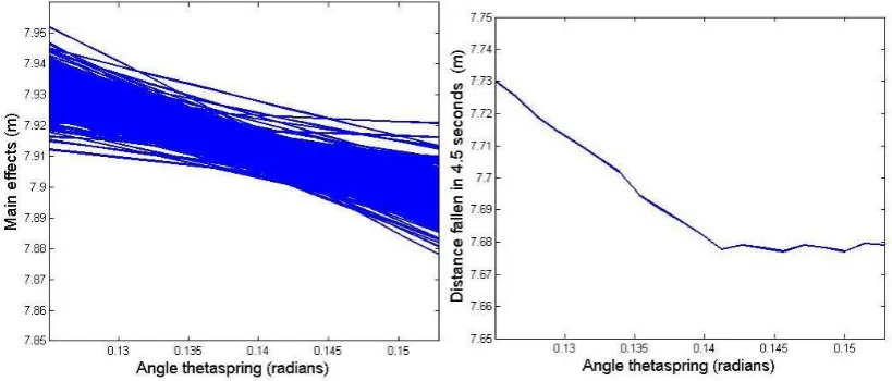
Figure 8 shows that plotting the main effects can obscure a local nonlinearity in the response to a change in a parameter. While in the current case the model is fairly insensitive to the parameter, it does highlight the fact that when looking at the global behaviour it is possible to miss details in the local behaviour.

4.2 The second run of sensitivity analysis

Figure 5: Main effect plot and one at a time plot for the reaction spring stiffness.

Figure 6: Main effect plot and one at a time plot for the main spring stiffness.

Figure 8: Main effect plot and one at a time plot for the angle ”thetaspring”.

Figure 9: Extended main effect plot and one at a time plot for the combined friction force.

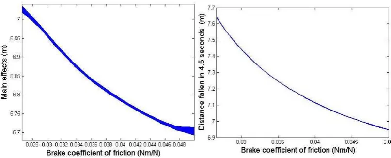
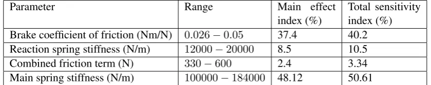
Table 3 shows the MEIs and TSIs from the second run of sensitivity analysis where fewer parameters were considered with an extended range. Again it can be seen that there is a relatively small contribution from the interactions. The results suggest that the most influential parameters are the brake friction coefficient and the main spring stiffness. However, it is not known how likely these parameters are to change, and by how much; it is not possible to truly state which are the most influential parameters without this information.

Figure 10: Extended main effect plot and one at a time plot for the main spring stiffness.

Figure 11: Extended main effect plot and one at a time plot for the reaction spring stiffness.

Parameter Range Main effect index (%)

Total sensitivity index (%) Brake coefficient of friction (Nm/N) 0.026−0.05 37.4 40.2 Reaction spring stiffness (N/m) 12000−20000 8.5 10.5 Combined friction term (N) 330−600 2.4 3.34 Main spring stiffness (N/m) 100000−184000 48.12 50.61

Table 3: Main effect index and total sensitivity index values from the second run of sensitivity analysis.

5

Conclusions

The aim of this paper was to develop a model of the AGR primary shutdown system and explore the use of probabilistic sensitivity analysis techniques on this model, with the objective of shedding light on the contribution of parameters to model uncertainty and the system’s performance. The results suggest that gaining a better understanding of the brake friction would be the most effective way of reducing the model uncertainty. However, it is impossible to definitively characterise the uncertainty of the model output without accurate estimates for how uncertain the input parameter values are. The results from the second round of sensitivity analysis imply that the system ought to be resistant to changes in several parameters at once; a component’s properties would have to change dramatically before the system becomes unsafe.

It is made clear in these results that while these global sensitivity analysis techniques use information from the entire range of the possible parameter space, they do not fully describe the model’s sensitivity to these parameters, because details (such as nonlinearities) can be lost when averaging over the other possible pa-rameters. This study has shown that it can be useful to show local sensitivity analysis results alongside the global ones as it provides context for comparison.

6

Acknowledgments

The Author would like to thank EDF Energy for funding the project and Marc Kennedy from the University of Sheffield Probability and Statistics Department for the use of GEM-SA.

References

[1] A. Saltelli, K. Chan, and E. M. Scott. Sensitivity Analysis. Wiley, 2000.

[2] P. Doubilet, C.B. Begg, M.C. Weinstein, P. Braun, and B.J. McNeil. Probabilistic sensitivity analysis using Monte Carlo simulation: A practical approach.Med Decis Making., 5:157–177, 1985.

[3] J. Helton. Uncertainty and sensitivity analysis techniques for use in performance assessment for ra-dioactive waste disposal. Reliability Engineering and System Safety, 42:327–367, 1993.

[4] G.J. McRae, J. W. Tilden, and J. H. Seinfeld. Global sensitivity analysis-a computational implementa-tion of the Fourier amplitude sensitivity test (FAST).Computers & Chemical Engineering, 6(1):15–25, 1982.

[5] A. Saltelli, S. Tarantola, and K. P.-S. Chan. A quantitative model-independent method for global sensitivity analysis of model output. Technometrics, 41:39–56, 1999. ISSN 0040-1706.

[7] J. Oakley and A. O’Hagan. Probabilistic sensitivity analysis of complex models: a Bayesian approach. Journal of the Royal Statistical Society, Series B, 66:751–769, 2002.

[8] P. L. Green. Bayesian system identification of nonlinear dynamical systems using a fast MCMC algo-rithm.European Nonlinear Oscillations Conference, 2014.

[9] P. L. Green and T. Baldacchino. Bayesian system identification in structural dynamics: Annealing with constant entropy variation. Probabilistic Engineering Mechanics (Under Review), 2014.

[10] K. Worden and W. Becker. On the identification of hysteretic systems. part ii: Bayesian sensitivity analysis.Mechanical Systems and Signal Processing, 29:213–227, 2012.