Development of a more energy efficient Roberts evaporator based on CFD modelling
76
0
0
Full text
(2) Development of a more energy efficient Roberts evaporator based on CFD modelling by. Steve Pennisi. November 2004. for the degree of Doctor of Philosophy in the School of Engineering James Cook University.
(3) Statement of Access. I, the undersigned, the author of this thesis, understand that James Cook University will make it available for use within the University Library and, via the Australian Digital Theses network, for use elsewhere. I understand that, as an unpublished work, a thesis has significant protection under the Copyright Act and I wish this work to be embargoed until Dec 2006.. Signature. Date.
(4) 11. Abstract. The evaporator station within a sugar mill is the single largest consumer of low pressure steam for heating purposes.. Factories have identified the need to reduce the energy. requirements of the evaporator station so that larger quantities of energy can be used for cogeneration and other purposes. The design of evaporator vessels has remained unchanged since the 1950s and most alterations and design improvements made during the time since have lacked the insight afforded by such tools as CFD modelling.. CFD model predictions allow for an. understanding of the fluid flow behaviour which is occurring inside the vessel and can not the visualised by any other means. The ability to visualise the behaviour of the entire flow field has been identified as the possible starting point for a novel design of evaporator and significant improvements in performance. As a result of this investigation a large number of data was gathered from factory vessels for comparison with CFD model predictions. There data did not previously exist in the literature in any suitable form . The factory data was used as part of the process to develop a CFD model capable of accurately predicting the fluid flow behaviour inside an evaporator vessel. The subsequent application of the CFD model concluded that the existing design of evaporator vessels contained significant deficiencies in the fluid flow behaviour and that incremental changes to geometry are not likely to produce significant improvements in performance. A novel design of evaporator is presented that has been developed using the CFD model predictions. The novel design significantly improves the fluid flow behaviour inside the vessel and a greater than 30% improvement in heat transfer performance is predicted. Despite the success of the CFD modelling included in this study, a number of areas for further investigation have been identified. These include improvements to the experimental procedure used to gather the factory data, improvements to be made to the CFD modelling tools developed to date and practical issues associated with implementation of the novel evaporator design..
(5) III. Acknowledgements. The author wishes to thank the following people and organisations for their valuable contributions: Dr 10ng-Leng Liow whose knowledge in the field of fluid dynamics has been invaluable to me. Dr Ross Broadfoot for going above and beyond the call of duty. The advice you gave was so much more than just standard supervision. Dr Philip Schneider for assistance of all things experimental. Dr Darrin Stephens for his knowledge of numerical modelling and for the long discussions we had. Mr Craig Muddle for his assistance and his tireless efforts when we were conducting the factory experiments. Sergeant Mark Retallick for all the time we spent drinking coffee, talking garbage and generally letting go of life's stresses. Duty First. The Sugar Research Institute (SRI) for their financial support to the project and for allowing me the opportunity to complete this project. The Australian Research COllllcil (ARC) for their financial support. The Queensland Government Department of State Development (QDSD) for their financial contribution..
(6) IV. Electronic copy. I, the undersigned, the author of this work, declare that the electronic copy of this thesis provided to the James Cook University Library is an accurate copy of the print thesis submitted, within the limits of the technology available.. Signature. Date.
(7) v. Statement of Sources. I declare that this thesis is my own work and has not been submitted in any form for another degree or diploma at any university or other institution of tertiary education. Information derived from the published or unpublished work of others has been acknowledged in the text and a list of references is given. I would like to acknowledge the contributions of Dr 10ng-Leng Liow and Dr Philip Schneider to the accompanying coauthored paper.. Signature. Date.
(8) VI. Contents Nomenclature ... ..................................................................... xiii 1.. Introduction ............................................................................................. 1 1.1. 1.2. 1.3. 1.4 1.5. 1.6. Types of evaporator vessels .. ..... .... ... ..... ...... ..... ...... ...... ...... ..... ...... ........ ...... ..... .. . 5 1.1.1 Plate type evaporators ........... ............ ........... ......... .............. ..... ......... ..... 5 1.1.2 Tube type evaporators ...... ....... ..... .. ......... ....... ..... .. ............ ...... ..... .. .. ..... . 7 Evaporator set operation ..... .. .... ..... ..... ... .... .. .... ..... ..... .. ...... .................. .. .... .. .... .. 10 1.2.1 General principles ....... ....... .... .... .. .. ... ........ .... .... .. .. ... ..... .. .... .... .. .. .. ..... ... 10 1.2.2 Co-generation .... ...... ... ........ ...... ...... ........... ...... ...... ........... ........ ...... ... ... 12 The Roberts vessel.. ..... .. ..... .. ......... ....... ..... .. ............ ......... .. ............ ...... ..... .. .. .... 16 1.3.1 The basic design ......... ........... ......... .............. ......... .............. ..... ......... ... 16 1.3.2 Vapour side operation .. .... ... ..... ...... ..... ...... ...... ...... ..... ...... ........ ...... ... ... 16 1.3.3 Juice side operation ..... ..... ...... ............ ..... ...... ........................... .... ...... .. 19 Evaporator performance .... ... .. ........ .... ... .... .. .. ........ .... ... .... .. .. .......... .... .. .... ... .. .... 23 Numerical modelling ...... ...... ... ........ ...... ...... ........... ...... ...... ........... ........ ...... ... ... 27 1.5.1 Steindl and Ingram ..... ........... ......... .............. ......... .............. ..... ......... ... 27 1.5.2 Stephens ...... .... .. ..... .. .. ....... ....... ..... .. ............ ...... ..... .. .......... ...... ..... .. .. .... 32 1. 5.3 Evaporator modelling .. ..... ..... ... .... .. .... ..... ..... .. ...... .................. .. .... .. .... .. 32 Summary ... .. ... ..... .. .... .... .. .. .. ..... ....... .... .... .. .. ... ..... .. .... .... .. .. .. ....... .. .... .... .. .. .. ..... ... 33. 2.. Objectives ............................................................................................... 35. 3.. Factory experiments ............................................................................. . 36 3.1 3.2 3.3 3.4 3.5 3.6 3.7 3.8. Introduction ............... ..... ......... ........... ......... .............. ..... .... .............. ..... ......... ... 36 The Proserpine #4 evaporator vessel.. ... ...... ......... ........ ...... ..... ...... ........ ...... ... ... 36 The Farleigh #2 evaporator .... ........ .... .. .... ... .. ........ .... ... .... .. .. .......... .... .. .... ... .. .... 38 Experimental equipment.. ...................... .... ...... ..... ...... ........................... .... ...... .. 40 Experimental procedure .. ...... ......... ........ ...... ......... ........ ...... ..... ...... ........ ...... ... ... 45 Experimental results ....... ......... ........... ... ......... ........... ......... .............. ..... ......... ... 48 Possible errors ......... .... .. ..... .. .. ....... ..... .. ..... .. ............ ...... ..... .. ......... ....... ..... .. .. .... 51 Discussion of experimental results ..... .. ....... .... ..... ..... .. ...... .................. .. .... .. .... .. 53 3.8.1 Inlet and outlet juice temperatures .... ....... .... .... .. .. ... ..... .. .... .... .. .. .. ..... ... 53 3.8.2 Temperature distribution ..... ... .. .... .. .... ..... ..... .. ...... .................. .. .... .. .... .. 54 3.8.3 Brix distribution .... .. .. ....... ..... .. ..... .. ......... ....... ..... .. ............ ...... ..... .. .. .... 54 3.9 Data used for CFD modelling ............. ......... .............. ......... .............. ..... ......... ... 55 3.10 Summary offactory experiments .. ........ ...... ......... ........ ...... ..... ...... ........ ...... ... ... 57. 4.. Numerical modelling ............................................................................. 58 4.1 4.2 4.3 4.4 4.5. Introduction ............... ... .. .... .. .... ..... ..... .. ...... ....................... .................. .. .... .. .... .. 58 The software package ... .. .. .. ..... ....... .... .... .. .. ... ........ .... .... .. .. ... ..... .. .... .... .. .. .. ..... ... 58 Model description ... ... ..... ...... ........... ...... ...... ........... ...... ...... ........... ........ ...... ... .. . 59 Governing equations .... .. .... ... .. ........ .... ... .... .. .. .......... ..... .... .. .. .......... .... .. .... ... .. .... 60 Fluid properties .......... ..... ......... ........... ......... ....................... .............. ..... ......... ... 62.
(9) Vll. 4.6 4.7. 4.8 4.9 4.10 4.11 4.12 4.13. 5.. Model validation results ........................................................................ 78 5.1 5.2 5.3 5.4 5.5 5.6. 6.. 4.5.1 Fluid temperature .... ... ........ ...... ...... ........... ...... ...... ........... ........ ...... ... ... 62 4.5.2 Sugar concentration ... ....... ....... ..... .. ......... ....... ..... .. ............ ...... ..... .. .. .... 62 Boundary conditions .. ..... ......... ........... ......... ....................... .............. ..... ......... ... 63 Geometrical considerations .. ......... ........ ...... ..... .... ... ..... ...... ..... ...... ........ ...... ...... 64 4.7.1 The calandria ..... .... ...... ..... ...... ....... ..... ..... ...... ........................... .... ...... .. 64 4.7.2 Flow constraint ..... ... .. ........ .... ... .... .. .. .......... .... .. ... .. .. .......... .... .. .... ... .. .... 65 4.7.3 The gaseous phase ... ... ........ ...... ...... ........... ........ .... ........... ........ ...... ... ... 67 Heat flow inside the calandria .......... ..... ......... ........... ......... .............. ..... ......... ... 69 Fluid flow above the calandria ....... ...... ..... .. ......... ....... ..... .. ............ ...... ..... .. .. .... 71 Turbulence modelling ... .. .... .. .... ..... ...... .. .... .. .... ..... ..... .. ...... .................. .. .... .. .... .. 72 Convergence criteria .. ... .. .. .. ..... ....... ..... .. .. .. ..... ....... .... .... .. .. ... ..... .. .... .... .. .. .. ..... ... 73 Meshing of the geometry ...... ... ........ ...... ...... ........... ...... ...... ........... ........ ...... ... ... 74 4.12.1 Mesh independence .......... .... ... .... .. .. .......... .. ... .... .. .. .......... .... .. .... ... .. .... 74 Summary of the numerical model .... ..... ......... ........... ......... .............. ..... ......... ... 77. Introduction ............... ... .. .... .. .... ..... ..... .. ...... .................. .. ... ............... ... .. .... .. .... .. 78 Validation procedure ... .. ..... .. .. ....... ..... .. ..... .. .. ....... ..... .. ..... .. ............ ...... ..... .. .. .... 78 Validating the juice brix and temperature distribution .. .. .. ... ..... .. .... .... .. .. .. ..... ... 79 Discussion of the juice brix and temperature validation .... ........... ........ ...... ... ... 82 Validating the heat flow predictions ... .. .... ... .. ........ .... ... .... .. .. .......... .... .. .... ... .. .... 83 Summary ofthe model validation results ... ..... ..... ...... ........................... .... ...... .. 85. Model prediction results ....................................................................... 86 6.1 6.2. 6.3. 6.4. 6.5. 6.6. 6.7. Introduction ............... ... .. .... .. .... ..... ..... .. ...... ............... ... .. ... ............... ... .. .... .. .... .. 86 Proserpine #4 ........... .... .. ..... .. .. ....... ....... ..... .. ............ ...... ..... .. .......... ...... ..... .. .. .... 87 6.2.1 CFD model details ...... ........... ......... .......... .... ......... .............. ..... ......... ... 87 6.2.2 Circulation patterns ...... .... .... .... ...... ..... .... ... ..... ...... ..... ...... ........ ...... ...... 88 6.2.3 Residence time distribution ...... .... ...... ..... ...... ........................... .... ...... .. 92 Farleigh #2 ................. ..... .... ...... ..... ...... ........................... ....................... .... ...... .. 93 6.3.1 CFD model details ... ..... .... ... ..... ...... ..... ....... ..... ...... ..... ...... ........ ...... ...... 93 6.3.2 Circulation patterns .... ........... ... ......... ........... ......... .............. ..... ......... ... 93 Deficiencies in the existing vessel design ... .. ....... ....... ..... .. ............ ...... ..... .. ... ... 99 6.4.1 Modifications to the existing design ....... ..... .. ...... .................. .. .... .. .... 100 6.4.2 Modifications considered ...... .... .. .. ... ........ .... .... .. .. ... ..... .. .... .... .. .. .. ...... 100 Modified Farleigh #2 ...... ...... ... ........ ...... ...... ........... ...... ...... ........... ........ ...... ... . 103 6.5.1 CFD model details ... .. ....... ....... ..... .. ......... ....... ..... .. ............ ...... ..... .. .. .. 103 6.5.2 Circulation patterns .... ........... ... ......... ........... ......... .............. ..... .......... 104 6.5.3 Heat transfer performance .... .... ...... ..... .... ... ..... ...... ..... ...... ........ ...... ... . 109 Novel evaporator design ..... ...... ..... ...... ................. ...... ........................... .... ..... . 110 6.6.1 Details ofthe design .. ........ .... ... .... .. .. ........ .... ... .... .. .. .......... .... .. .... ... .. .. 110 6.6.2 CFD model details ... ... ........ ...... ...... ........... ...... ...... ........... ........ ...... ... . III 6.6.3 Circulation patterns .... ........... ... ......... ........... ......... .............. ..... .......... 113 6.6.4 Heat transfer performance ..... .. ..... .. ......... ....... ..... .. ............ ...... ..... .. .. .. 115 Summary of model predictions ..... ..... ... .... .. .... ..... ..... .. ...... .................. .. .... .. .... 116.
(10) Vlll. 7.. Summary, conclusions and recommendations .................................. 118 7.1 7.2 7.3. Factory experiments .... .. ..... .. .. ....... ..... .. ..... .. .. ....... ..... .. ..... .. ............ .... .. ..... .. .. .. 118 CFD model development .... .. .... ..... ..... .. ...... ..... ..... ..... .. ...... .................. .. .... .. .... 119 CFD model application ... .. .. ..... ....... .... .... .. ...... ....... .... .... .. .. ... ..... .. .... .... .. .. .. ...... 120. References ............................................................................ 123 Appendix A - Glossary of terms ................................................. 126 Appendix B - Example heat and mass balance calculations ............... 128 Appendix C - CFX input file ...................................................... 131 Appendix D - Fluid property equations ........................................ 145 Appendix E - Proserpine #4 residence time distribution ................... 146.
(11) IX. List of figures Figure 1.1 Figure Figure Figure Figure Figure. 1.2 1.3 1.4 1.5 1.6. Figure 1.7 Figure 1.8 Figure 1.9 Figure 1.10 Figure Figure Figure Figure. 1.11 1.12 1.13 1.14. Figure 1.15 Figure 1.16 Figure 1.17 Figure 1.18. Figure 3.1 Figure 3.2 Figure 3.3 Figure 3.4 Figure 3.5 Figure 3.6 Figure 3.7 Figure 3.8 Figure 3.9. Australian sugar industry regions, Queensland Sugar Corporation (2001) ..................... ..... .... ...... ..... ...... ...................... ..... .... ...... ..... ... ..... .... ...... ..... 4 The process of raw sugar production ....... ..... ...... ...... ...... ..... ...... ........ ...... ......... 5 Alfa Laval plate heat exchanger, Alfa-Laval (2001) ....... .............. .............. ...... 6 Typical plate type falling fihn evaporator, Grant et al. (2000) ... .... .. .... ... .. ....... 7 Typical Roberts design of evaporator, Watson (1987) .... ..... ...... ... ..... ...... ... ...... 8 Material and power requirements for various evaporator types, Lehnberger (1996) ..... .. .... .. .... ..... ..... .. ...... ............... ... .. ... ............... ... .. .... .. .... ..... 9 Multiple effect evaporation diagram, Wright (1983) .... .. ... ......... ...... ..... .. .. ..... 10 A typical evaporator brix profile, Attard (1991) .... ......... .............. .............. .... 12 Generalised evaporatoriheater/vacuum pan vapour system for improved LP steam economy, Wright (2000) .... .... ... ...... .. .......... .... .. .... ... .. ..... 15 Steam lane and baffle design in Roberts evaporator vessels, Peacock (1999) ....... ..... ...... ........ ...... ... ...... .... .... ...... ..... ...... ........ ...... ... ...... ........ ...... ... .... 17 Types ofbaffies in Roberts evaporator vessels, Peacock (1999) ................ .... 17 Variable tube pitch calandria, Tromp (1966) .... ..... .. ....... .. .......... .... .. ..... .. .. ..... 18 A circumferential belt producing radial vapour flow, Peacock (1999) .... ... .... 19 Plot of juice head above the calandria versus level of juice in the tubes, Watson (1986a) ..... .. .... ..... ..... .. ...... ............... ... .. ... ............... ... .. .... .. .... ... 22 Plot ofHTC with and without downtakes, Watson (1986a) ....... .... .. ..... .. .. ..... 22 Predicted velocity profile for an evaporator vessel with peripheral feed and a central outlet, Steindl and Ingram (1999) .. .... ..... ...... ........ ...... ... .... 30 Predicted brix profile for an evaporator vessel with peripheral feed and a central outlet, Steindl and Ingram (1999) ...... ...................... ..... .... ...... ... 31 Predicted variation of the local evaporation rate with radial position for an evaporator vessel with peripheral feed and a central outlet, Steindl and Ingram (1999) ... ....... ..... .. ....... .. ....... ..... .. ....... .. .......... .... .. ..... .. .. ..... 31 Schematic of the vapour side operation of the Proserpine Mill evaporator station .. .... .. .. .. ..... ....... .... .... .. .. ... ........ .... .... .. .. ... ..... .. .... .... .. .. .. ..... .... 37 Schematic of the juice side operation of the Proserpine Mill evaporator station ..... .. ..... .. .. ....... ..... .. ....... .. ....... ..... .. ....... .. .......... .... .. ..... .. .. ..... 37 Schematic of the vapour side operation of the Farleigh Mill evaporator station ........ ...... ... ...... .... .... ...... ... ...... .... .... ...... ..... ...... ........ ...... ... .... 40 Schematic of the juice side operation of the Farleigh Mill evaporator station ....... .. .......... .... .. .... ... .. ........ .... ... ...... .. .......... .... .. ..... .. .......... .... .. .... ... .. ..... 40 Location of tapping points installed in the bottom of the Farleigh #2 vessel when viewed from above .. .... ......... .......... .... ......... .............. .............. .... 41 Location of tapping points installed in the bottom of the Proserpine #4 vessel when viewed from above ... ...... .......... ..... .. ...... ............... ... .. .... .. .... ... 41 A side view of a sample probe positioned inside a vessel... ... .. .... .... .. .. .. ..... .... 42 Photograph of a sampling probe ... ... ... ...... ..... ...... ... ... ...... ..... ...... ... ..... ...... ... .... 43 Plot of juice flow rate at the inlet to the Proserpine #4 vessel for test no. 3 .......... .............. .............. ........... ......... .............. .............. ....................... .... 47.
(12) x. Figure 3.10 Plot of headspace and calandria pressures in the Proserpine #4 vessel for test no. 3 .......... .... .. ..... .. .. ....... ..... .. ....... .. .......... .... .. ..... .. .. ........ .... .. ..... .. .. ..... 47 Figure 4.1 Plot of friction factor versus Reynolds Number. .... ......... .............. ..... ......... .... 66 Figure 4.2 Plot of the velocity errors relative to the "very fine" mesh .. .................... ..... .. 76 Figure 4.3 Plot of the brix errors relative to the "very fme" mesh ...................... .... ......... 76 Figure 6.1 Mesh applied to the Proserpine #4 geometry ..... .... ... ...... .. .......... .... .. .... ... .. ..... 87 Figure 6.2 Vector plot on a vertical plane through the centre of one of the juice inlets for the Proserpine #4 vessel... ......... .............. ......... .............. ..... ......... .... 88 Figure 6.3 Close up vector plot ofthe juice flow around the inlet from Figure 6.2 .... ..... 89 Figure 6.4 Juice brix plot on a vertical plane through the centre of one juice inlet for the Proserpine #4 vessel... ...... .... .... .... ... ..... .. .... .... ..... ... ..... .. .... .... ........ ... .... 90 Figure 6.5 Juice brix plot on a horizontal plane 50 mm below the distribution plate for the Proserpine #4 vessel... .... ...... .. ........ .... ... ...... .. .......... .... .. .... ... .. ..... 91 Figure 6.6 Mesh applied to the Farleigh #2 geometry .. ........... ......... .............. ..... ......... .... 93 Figure 6.7 Vector plot on a vertical plane through the centre of one of the juice outlets for the Farleigh #2 vessel... ..... .... ........... .... ........................ ..... .... ......... 94 Figure 6.8 Pressure plot on a vertical plane through the centre of one of the juice outlets for the Farleigh #2 vessel... .. ... ...... ... ........ ... ... ...... ..... ...... ... ..... ...... ... .... 95 Figure 6.9 Close up vector plot of the juice flow around the inlet from Figure 6.7 .. ... .... 96 Figure 6.10 Juice brix plot on a vertical plane through the centre of one of the juice outlets for the Farleigh #2 vessel... .. ......... ..... .. ...... ............... ... .. .... .. ....... 96 Figure 6.11 Close up juice brix plot of the flow around the inlet from Figure 6.9 ...... ... .... 97 Figure 6.12 Vector plot on a horizontal plane through the centre of the juice inlet pipe for the Farleigh #2 vessel .... .... ... ...... .. ........ .... ... ...... .. .......... .... .. .... ... .. ..... 98 Figure 6.13 Juice brix plot on a horizontal plane through the centre on the juice inlet pipe for the Farleigh #2 vessel ......... ..... .... .... .... ...... ..... ...... .............. ..... .. 98 Figure 6.1 4 Top view of the modified calandria layout for the Farleigh #2 vessel... ....... l0l Figure 6.15 Side view of the modified juice inlet and outlet system for the Farleigh #2 vessel ... ..... ...... ... ........ ... ... ...... ..... ...... ... ... ...... ..... ...... ... ..... ...... ... .. 102 Figure 6.16 Details of the holes in the modified juice inlet manifold for the Farleigh #2 vessel ... ... .. .... .. ......... ..... .. ...... ............... .. ...... ............... ... .. .... .. ..... 102 Figure 6.17 Mesh applied to the modified Farleigh #2 geometry ...... .. .......... .... .. ..... .. .. ... 104 Figure 6.18 Juice brix plot on a vertical plane through the centre of the wedge for the modified Farleigh #2 geometry .... ...... ... ........ ... ... ...... ..... ...... ... ..... ...... ... .. 105 Figure 6.19 Vector plot on a vertical plane through the centre of the wedge for the modified Farleigh #2 geometry ..... ..... .... ........... .... ........................ ..... .... ....... 106 Figure 6.20 Juice brix plot on a horizontal plane through the centre of the juice inlet manifold for the modified Farleigh #2 geometry .... .............. ..... ......... .. 107 Figure 6.21 Vector plot on a horizontal plane through the centre of the juice inlet manifold for the modified Farleigh #2 geometry ... ... ...... ..... ...... ... ..... ...... ... .. 108 Figure 6.22 Details of each cell in the linear design .... ... ....... .... .... .... ... ..... .. .... .... ........ ... .. III Figure 6.23 Mesh applied to one cell ofthe linear evaporator geometry ......... ... .. .... .. ..... 112 Figure 6.24 Vector plot on a vertical plane inside one cell of the linear evaporator. .. .. ... l13 Figure 6.25 Juice brix plot on a vertical plane inside one cell of the linear evaporator ...... ...... ... ..... ...... ... ........ ... ... ...... ..... ...... ... ..... .... ..... ...... ... ..... ...... ... .. 114.
(13) Xl. Figure 6.26 Juice brix plot on a vertical plane inside the three second effect cells of the linear evaporator. ................................................................................. 115 Figure 6.27 Juice brix plot on a vertical plane inside the four fourth effect cells of the linear evaporator ...................................................................................... 115.
(14) Xli. List of tables Table 1.1 Table 3.1 Table 3.2 Table 3.3 Table 3.4 Table 3.5 Table 3.6 Table 3.7 Table 3.8 Table 3.9 Table 3.10 Table 3.11 Table 3.12 Table 3.13 Table 3.14 Table 4.1 Table 4.2 Table 4.3 Table 5.1 Table 5.2 Table Table Table Table. 5.3 5.4 5.5 5.6. Typical values ofHTC for different effects (Watson 1986) .................... .. ..... 23 Sampling probe vertical locations for tests conducted on the Proserpine #4 vessel ...................................... ............ .. ......... ............ .. ............. 43 Sampling probe vertical locations for tests conducted on the Farleigh #2 vessel ................. .. ......... .. ....... ... .. ....................... .. ......... .. .......... .. ......... .. ..... 43 Summary of data from the Proserpine #4 vessel .... .............. ...... .. ............ .... ... 48 Summary of data from the Farleigh #2 vessei.. .. .. .. .... .. .. .... .... .. .... .... .. .. .... .. .. ... 49 Results of heat balance calculations on the Proserpine #4 vessel .... ...... .. .... ... 50 Results of heat balance calculations on the Farleigh #2 vessei.. ............ .. .. ..... 50 Estimated and measured juice temperatures at the inlet of the Proserpine #4 vessel .......... .... ...... .... ............ .. ...... .. ............ ... ...... .. ............ .... ... 53 Estimated and measured juice temperatures at the inlet of the Farleigh #2 vessel ...... .......... ..... ........... ...... ...... ..... ..... .......... ..... ........... ....... ..... ........... ... 54 Summary of vertical locations of the sampling points used for the Proserpine #4 vessel .......... .. ....... ... .. ............ .. ........ ............ ... ........ ............ .. ..... 55 Summary of vertical locations of the sampling points used for the Farleigh #2 vessel .. ............ .... ...... .... ............ .. ...... .. ............. .. ...... .. ............ .... ... 55 Summary of data used as boundary conditions for the CFD model of the Proserpine #4 vessel .... .... ...... .... .. ...... .... .......... .... ........ ............ ............ .... .. 56 Summary of data used as boundary conditions for the CFD model of the Farleigh #2 vessel ........ .. ....... ... .. ............ .. ....... .. ............ .. ........ ............ .. ..... 56 Summary of data used for comparison with the CFD model of the Proserpine #4 vessel .......... .. ....... ... .. ....................... .. ......... .. .......... .. ......... .. ..... 56 Summary of data used for comparison with the CFD model of the Farieigh #2 vessel .......................................... ....................... ........................... 57 Summary of the inlet boundary conditions for the CFD model of the Proserpine #4 vessel ........ .. .. ....... ... .. .. ..................... .. ....... .. .. .......... .. ....... .. .. ..... 63 Summary of the inlet boundary conditions for the CFD model of the Farleigh #2 vessel ... ... .. .. .... .. .. ...... .. .. .... .. .. ... .. .. .... .. .. .. .. .. .. ... .. .. .... .. .. ... .. .. .... .. .. ... 63 Calculated errors from different mesh densities .... ............ ............ ............ .... .. 75 Measured and predicted juice temperature data from the Proserpine #4 vessel ...... .. ........ ............ .. ....... ... .. ............ .. ........ ............ .. .. .. ..... ............ .. ..... 79 Measured and predicted juice temperature data from the Farleigh #2 vessel ...................... ..... .......... ..... ...... ...................... ..... .......... ........ ..... .......... ... 80 Measured and predicted juice brix data from the Proserpine #4 vessel ... .. ..... 81 Measured and predicted juice brix data from the Farleigh #2 vesseL .......... .. 81 Measured and predicted heat flow data from the Proserpine #4 vessel .... .. .... 84 Measured and predicted heat flow data from the Farleigh #2 vessel .............. 84.
(15) X1ll. Nomenclature A. Heating surface area of an evaporator vessel (m2 ) Open area ratio of the tube-plate. B. Brix (%) Juice brix at the inlet of the vessel (%) Juice brix at the outlet of the vessel (%). Cp,. Specific heat capacity of the liquid phase (J.kg·1 .K 1) Surface-fluid constant used in the Rohsenow (1952) equation for heat transfer Constant used in the k - s turbulence model (1 .44) Constant used in the k - s turbulence model (1.92). DS. Dry substance by mass (%). HTR. Heat transfer ratio. I. W. Ratio of impurities to water concentration by mass. Ja. . . Iess Jacob Numb er, d efime d as: --'--'--'---"""!' Cp(T, - T,at ) DlmenslOn hrg. K. Von Karman constant (0.417). p. Purity (%) Turbulence production due to. Pr. VISCOUS. and buoyancy forces, used in the k - s. Dimensionless Prandtl Number, defined as: CPJl, K,.
(16) XIV. Q. Total heat flow through the calandria (W). Q,. Heat flow through the calandria causing evaporation (W) Heat flow through the calandria as a result of condensation (W). Q,. Heat flow through the calandria causing sensible heating of the liquid phase (W). Re. Reynold's number. s w. Ratio of sucrose to water concentration by mass Additional mass source tenn in the continuity equations (kg·mTs·l ) Additional energy source tenn in the energy equations (J·m·3 ·S·l ) Additional momentum source tenn in the momentum equations (kg.m·2.s· 2). T. General fluid temperature (K). T,. Boiling point elevation temperature (BPET) at atmospheric pressure (K). T,. Boiling point elevation temperature (BPET) at a given pressure (K). T,. Juice temperature at the outlet of the vessel (0C). T,. Saturation temperature of water at pressure under consideration (K). u. Vessel average heat transfer coefficient (HTC) (W·m·2 K. l. ). Typical Australian vessel average heat transfer coefficient (HTC) (W·m·2·K l ). v. Velocity vector for general fluid (m·s·l ). v. Average component of velocity in turbulent flow (m·s· l ). v'. Fluctuating component of velocity in turbulent flow (m·s· l ).
(17) xv. V+. Dimensionless near wall velocity. Vg. Velocity vector for the gas phase (m·s· l ). V;. Velocity vector for the liquid phase (m·s· l ). Wg. Mass flow rate of vapour (kg·s· l ). W,. Mass flow rate ofliquid (kg·s· l ). X. Mass fraction of vapour present in a given volume of fluid (fluid quality). Yg. Volumetric flow rate of vapour (mJ·s·l ). 1';. Volumetric flow rate ofliquid (mJ·s· l ). d. Internal diameter of the heating tubes (m). e. Enthalpy (kJ.kg·l). f. Friction factor as applied in the Colebrook equation. g. Acceleration due to gravity (9.81 m·s·2). hlg. Latent heat of evaporation (J·kg· l ). hg. Enthalpy of the gas phase (kJ.kg"l). hi. Enthalpy of the liquid phase (kJ·kg·l ). k. Turbulence kinetic energy, used in the k - [; turbulence model (m 2·s·2). k,. Kinematic diffusivity ofbrix in solution (m2·s·l ). m,. Mass flow rate of vapour produced by evaporation (kg·s·l ). m,. Mass flow rate of condensate out of the calandria (kg·s· l ).
(18) XVI. m". Mass flow rate of juice at the inlet of the vessel (kg·s· l ). m om. Mass flow rate of juice at the outlet of the vessel (kg·s·l ). n. Fluid constant used in the Rohsenow (1952) equation for heat transfer. p. Pressure (Pa). qg. Heat flow into the gas phase (W). q,. Heat flow into the liquid phase (W). t. Time (s). y+. Dimensionless distance from the wall. t'!T. Effective temperature difference between the heating fluid and the heated fluid (K). ag. Volume fraction of gas phase. a,. Volume fraction of liquid phase Turbulence eddy dissipation, used in the k - s turbulence model (m2 ·s·'). rp. Any specific variable in the vector equations. K,. Thermal conductivity of the liquid phase (W·m·I .K'I) General fluid viscosity (Pa·s). Pg. Viscosity of the gas phase (Pa·s). P,. Viscosity ofthe liquid phase CPa·s). Pm. Average fluid viscosity based on fluid quality (Pa·s). PI. Turbulence viscosity, used in the k - s turbulence model CPa·s).
(19) XVII. o3. P. Density of general fluid (kg om. Pg. Density of the gas phase (kg om. PI. Density of the liquid phase (kg om. Pm. Average fluid density based on fluid quality (kg m. Tm. Wall shear stress (Pa). a-k. Constant used in the k. a-I. Surface tension of the liquid phase (Nomoi). a-,. Constant used in the k -. ). 03. ). o3. ). o. - li. li. turbulence model (1. 0). turbulence model (1.3). o3. ).
(20) 1. Chapter 1 Introduction. 1.. Introduction. Sugar is Australia's second largest export crop and Queensland's largest agricultural commodity. Queensland currently produces approximately 95% of Australia's raw sugar with the remainder produced in New South Wales and Western Australia. In Australia, 520,000 hectares of land are currently under cane and this area is increasing, particularly in the Burdekin, Herbert, Tully and Proserpine regions. Figure 1.1, from Queensland Sugar Corporation (2001) , gives an overview of the sugar industry regions around Australia. Australia produces raw and refined sugars both for export and internal consumption. In order to clarify the many industry specific terms, a glossary of terms is provided in Appendix A. The majority of the terms seen in Appendix A were obtained from Stephens (2001) and Bureau of Sugar Experiment Stations (BSES) (1992). Figure 1.2 shows the manufacturing process involved in the production of raw sugar. The numbers shown on Figure 1.2 correspond to the steps detailed as follows: 1.. Growing, Cane grown in the field is harvested using mechanical harvesters and transported to the factory on a small gauge railway system.. 2.. Shredding, The cane is weighed and dumped onto a conveyor belt and then passed through a shredder to form a coarse pulp. The shredder breaks open the fibrous cells and makes the juice more accessible to be extracted. Upon leaving the shredder the pulp is known as prepared cane.. 3.. Milling, The prepared cane is squeezed in a sequential series of grooved rolls. This process is known in the industry as milling. The juice is removed from the bottom of the mills and the fibre (bagasse) is passed to the next milling stage for further squeezing. Most factories employ four or five milling stages and use counter-current washing, with water and juice, in the mills to maximise the removal of sucrose from the cane cells.. 4.. Bagasse storage,. The bagasse exiting the final milling stage is stored in. stockpiles and returned to the factory's boiler station as fuel for combustion. The boiler station provides high-pressure steam for turbine drives on the shredder, mills and the turbo-alternators.. Factories produce electricity for. internal consumption and export small amounts of power to the state grid..
(21) 2. Chapter I Introduction 5.. Clarification. The juice extracted from the first and second milling stages is. combined and then heated with low-pressure (LP) steam from the exhaust of the turbines or vapour withdrawn from the evaporator station. Lime is added to adjust the pH to approximately 7.8 and to form a precipitate of calcium phosphate. This precipitate coagulates with mud (soil) particles to form floes that settle out in vessels called clarifiers. The mud removed in the clarification stage is processed through rotary vacuum filters to reduce the sucrose content contained in the mud. The mud cake from the filters is returned to the fields as mill mud. 6.. Juice storage. The clarified juice is passed to an intermediate storage termed. the Evaporator Supply Juice (ESJ) tank in order to buffer out any fluctuations in the juice supply. Some factories divert small quantities of clarified juice to other parts of the factory to replace the use of water and therefore reduce the loading on the evaporator stage. 7.. Evaporation. The ESJ is passed through a multiple effect evaporator station. that generally comprises quadruple or quintuple evaporators, Wright (1983). The evaporators boil off the majority of excess water contained in the juice, without supersaturating the sucrose mixture.. When referring to all of the. evaporator vessels the term "evaporator set" or simply "set" is used. The first evaporation stage is at a pressure slightly above atmospheric pressure (115 kPa abs) and the final stage is under vacuum (15 kPa abs). The operating pressure of each evaporation stage in the set decreases progressively from the first to the last stage. Each evaporation stage is known as an effect, each effect can consist of a single vessel or a number of vessels running in parallel. The first effect uses LP steam, from the exhaust of the turbines, as the heating source and subsequent effects use the vapour boiled off in the previous effect as the heat source. After the final stage of evaporation the juice is called syrup or liquor. 8.. Crystallisation. The syrup is boiled again under high vacuum (15 kPa abs) in. evaporative crystallisation pans. The boiling super-saturates the syrup and seed crystals are added to the liquid to initiate crystal growth.. The mixture of. crystals and liquid is now called massecuite. 9.. Fugalling.. The crystals are removed from the liquid by spinning the. massecuite at high speed in perforated baskets called centrifuges.. The.
(22) 3 Chapter 1 Introduction massecuite is separated into crystals and molasses.. The molasses is then. recycled and boiled again to recover more of the sucrose from the solution. Australian factories predominantly use the three-massecuite formula where the molasses is re-boiled three times. The first vacuum pan is called the ' A' pan, the second stage the 'B' pan and the third stage is the. 'c' pan, with the purity of. the massecuite boiled decreasing after each boiling. Molasses leaving the third stage is called final molasses and is predominantly used as cattle feed or as feedstock for fermentation. The sugar crystals produced in the third stage are not sent to product but are recycled to the A and B pans as seed, or are remelted and mixed with the syrup entering the A and B pan stages. 10. Drying, The raw sugar crystals produced by the A and B pans are dried by tumbling through a counter-current airflow in a rotary drum. The raw sugar product is then sent to storage bins to await shipment. 11. Co-generation, Sugar mills produce electricity for internal consumption by passing high-pressure steam from the bagasse-fired boilers through turboalternators. In some cases excess electricity is produced and exported to the state grid. This process is known as co-generation..
(23) 4. Chapter 1 Introdudi m. _ .. ,-_... - ."'''"-_. - .... _ __ .... J> _ A _. The. Australian Sugar Industry. -"". . ......... ~. _. ...... -C. ... ,~ .. _---_. -"-... ...... '.-••. t . - d~. ... •.....,~ .<,'~.--. _ _. .A. ............. Aft. ... "--'.". ~-. "..• ....-. f..,..- .. .... __ A. ....-.-~. c. ...... _. _ _A. _ ...- ..... OwoJ_'"_'''. .. ___ ........ .•••••••• , . -- •• •••••• • • ••••••••••• • -- •••• ---------- _.j Nlw IOUlH WA'H. , -. --- ... . .._. _. -~ ...... •. .,. .......-a::. •. ...... .........--. _. ... ._-... i.......... -',. .. "-'II. .......,. .... .. o..i. Figure 1.1 Auru-alian ougar mdmtry regl ffi s, Queensland Sugar COllloratim (2001). -.
(24) 5 Chapter 1 Introduction. 1. PRODUCTION OF RAW SUGAR. Harvesti ng. Snrlid08f Cane Tranopon. Fi gure 1.2 The process of raw sugar production. 1.1. Types of evaporator vessels. The Australian sugar industry utilises both plate and tube type vessels . Both the plate and the tube type vessels can operate as falling fihn or rising fihn mode. The falling or rising film designation is in reference to the direction of juice flow, e.g. the juice in a rising film tube type evaporator enters the vessel beneath the heating element and rises up through the vertical heating tubes or plates, due to the boiling action of the juice inside the tubes.. 1.1.1. Plate type evaporators. Plate type evaporators have a series of wafered plates packed together with the hot and the cold fluids on either side. The juice is boiled inside the plate pack and the liquid / vapour mixture passes through to the outlet. The advantages of the plate type evaporators are that they tend to be more compact than tube types, are easier to increase the heating surface area (HSA) and they tend to have higher heat transfer coefficient (HTC) and lower temperature differences than the tube type vessels. The disadvantages are that they are more expensive per unit HSA to install, are prone to increased scaling rates and for the gasketted types, are.
(25) 6 Chapter 1 Introduction more expensive to maintain. They also require more stringent control in order to maintain peak operational efficiency. Rising film plate type evaporators can be used as a booster in conjunction with another tube type vessel or as a stand-alone. When operating as a booster type vessel the outlet of the plate evaporator splits into two lines. The heavier liquid is withdrawn from the bottom and piped to the juice space of a tube type vessel and the lighter vapour is piped into the vapour space of the same vessel. When operating in this configuration the plate evaporator is said to be operating as a booster since it must have pipe connections to another Roberts type vessel operating under the same process conditions. Figure 1.3, from Alfa-Laval (2001), is an open in-line for assembly picture of an Alfa-Laval plate type, rising film evaporator used to operate as a booster.. Plate type evaporators can also operate as stand-alone in a. configuration whereby the heating plate pack is contained within a circular vessel for the containment of the juice and vapour. Figure 1.4, from Grant et al. (2000), shows a plate type, falling film evaporator with the heating plates inside a vapour recovery vessel.. Figure 1.3 Alfa Laval plate heat exchanger, Alfa-Laval (2001).
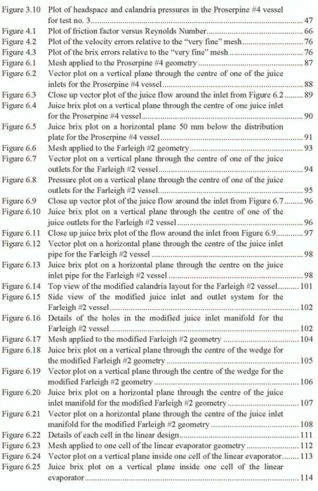
(26) 7. Chapter 1 Introduction. r---1;;;;•••-. Sugar Juice Vapour Channel. .... Steam. Juice Distribution. Heatillg steam. Vapour Channel. Sugar Juice. Figure 1.4 Typical plate type falling film evaporator, Grant et al. (2000). 1.1.2. Tube type evaporators. Tube type evaporators consist of a series of vertical tubes packed into a heating element called a calandria. Saturated LP steam or vapour condenses on the outside of the tubes while the juice boils on the inside. Tube type, falling film evaporators pump the juice onto a perforated plate above the tops of the tubes and force the juice and the vapour down the tubes. Tube type, rising film evaporators feed juice into the space beneath the calandria, allow the juice to boil inside the tubes and remove the concentrated juice from the bottom of the vessel. Vapour passes up the tubes and into the 'headspace' of the vessel. Similarly the pressure difference between vessels causes the vapour to flow from the headspace of one vessel to the calandria of the next. Figure 1.5, from Watson (1987), shows a typical design of the tube type, rising film evaporator. In the past, several variations of juice entry and exit locations above and below the calandria have been adopted. This gave rise to the terms under and over, when describing the location of the juice inlet and outlet locations, e.g. an under-over configuration would have the juice entry below the calandria and the juice exit above the calandria.. By far the most common evaporator in the Australian. industry is the tube type, rising film evaporator in the under-under configuration. This type of vessel is referred to in the industry as the 'Roberts' evaporator..
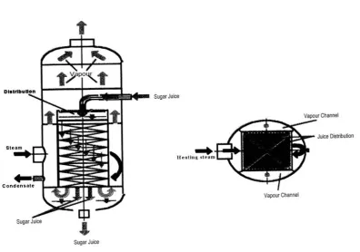
(27) 8 Chapter 1 Introduction. BaUles 1~. GASES. --+-.....,. JUICE r:::=~:...... ItU:T. __ JUICE run..ET. Figure 1.5 Typical Roberts design of evaporator, Watson (1987). Rural Press Q1d (1998) and Rural Press Q1d (2001) contain a breakdown of the Australian sugar industry's evaporative capacity in tenns of HSA.. The Australian sugar industry. 2. operates a total of approximately 423 000 m of evaporator HSA. Of this figure over 97% is in the fonn of the Roberts evaporator, with the remainder being plate type of various descriptions. Some Australian sugar mills use plate type heat exchangers to preheat the ESJ close to the boiling point before it enters the first evaporator vessel to reduce the amount of sensible heating required in the first effect of the evaporator station. Juice pre-heaters are not included in the scope of this investigation. The main advantages of the Roberts evaporators are the low cost per unit of HSA, the low maintenance costs, the ease of cleaning including mechanical cleaning if required and the robust control of these units due to the larger buffer volume of juice held in the base of these vessels. DeViana et al. (1993) states that the installed cost of a plate type evaporator.
(28) 9. Chapter 1 Introduction is typically in the range of $450/m 2 to $750/m 2 , depending on the particular installation requirements. Roberts vessels are typically installed for $350/m 2 to $450/m 2 . In spite of the reduced cost associated with the tube type Roberts evaporators, the material requirements of the tubular type vessels tend to be significantly higher. Figure 1.6a, from Lehnberger (1996), shows the material requirements for the construction of various evaporator types in kilograms of materials per unit ofHSA. 16. 30. ~. ~ Vessel (Steel). ::t:. ·c ::>. E. W. mr. t2iI Electrical power. :..... .. ~. 8. E. VI VI. Oi. rn. "§. 20. :..... . "'.". <C. ::t:. <C. rn. ~Heat losses. mlI (Stainless Heating surface steel). !!!. ""!!!. 10. CO". S. ;. :i!. D... 4. 0. 0 Robert Evaporator. 0. Climbing Film Plate Evaporator. Robert Evaporator. (a). (b). Figure 1.6 Material and power requirements for vanous evaporator types, Lehnberger (1996). The other major running cost associated with some evaporators is the electrical power required to drive pumps etc.. In most cases the Roberts design requires no pumping. capacity, as mentioned previously.. Figure 1.6b shows the power costs of various. evaporator types. The HTC of plate type evaporators is generally higher than tubular type evaporators. An increase in the HTC will allow lesser HSA to be installed for the same heat flux (evaporation rate). Thus the capital cost for a given evaporation duty may be reduced for plate evaporators by decreasing the amount of HSA required. This must be taken into account when considering the cost figures quoted previously in AS$/m2 ..
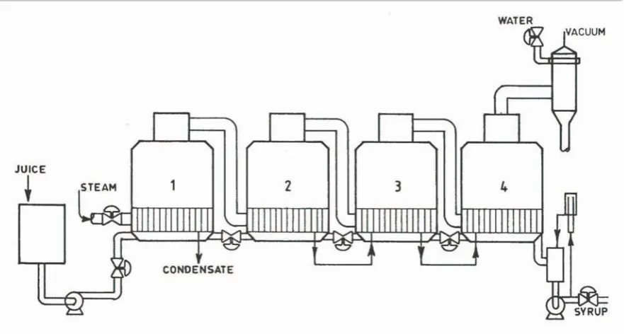
(29) 10 Chapter 1 Introduction. 1.2. Evaporator set operation. 1.2.1. General principles. Evaporator vessels are configured such that the vapour evaporated in the first effect is used as the heat source for the second effect and so on down the set. Figure 1.7 Wright (1983) shows this configuration pictorially. A temperature difference driving force is required to drive the heat transfer and so the temperature of the vapour at the outlet of the vessel will always be lower than that of the vapour or LP steam used as the heating source. The vapour is recycled in this manner to improve the thermal efficiency of the evaporator set. WATER. JUICE. t CONDENSATE. Figure 1.7 Multiple effect evaporation diagram, Wright (1983). The temperature difference is often used to judge the thermal efficiency of the vessels. LP steam is used as the heat source in the first effect, and is typically at 118°C to 125 °c in the saturated condition or very slightly superheated, whilst the temperature of the vapour at the outlet of the final effect is usually about 55 to 60°C at saturated conditions. The pressure in the first effect vessel is determined by the pressure of the LP steam supplied to the evaporator set and in most cases de-superheaters are used to ensure the LP steam is at saturated conditions. The saturation temperature of the vapour at the outlet of the final effect vessel is regulated by controlling the headspace pressure (vacuum) in the [mal effect vessel(s). Given that the vapour pressure is being controlled by the two extremes, at the.
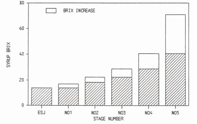
(30) 11. Chapter 1 Introduction first and last vessel(s) of the set, the pressure of the vapour streams in the remainder of the vessels in the set are left to equilibrate naturally. Many factors influence the equilibrium pressures and these include the heat transfer areas of the vessels in the set, the heat transfer coefficients (HTC), the vapour flow rates, and rates of withdrawal of vapour from individual vessels for other heating duties e.g. juice heating. Since the l880s the sugar industry has adopted the principle of multiple effect evaporation because it gives a more efficient usage of LP steam compared with the earlier practice of single vessel evaporation.. Wright (1983) states that the LP steam requirement for the. evaporation of unit mass of water is approximately (lin) units, where n is the number of stages. Therefore, LP steam consumption is reduced by the implementation of a larger number of evaporator stages. However, the heating surface area (HSA), and therefore the capital cost, to achieve the required evaporation capacity must increase as more stages are specified. This is due to the reduced temperature difference available across each stage and therefore reduced driving force for heat transfer, then available across each stage. The number of stages chosen is usually that just necessary to achieve the required LP steam economy.. The Rural Press Qld (200 1) contains data on the entire Australian sugar. industry's evaporator HSA.. From this data it can be calculated that, at the time of. publication, the Australian sugar industry had approximately 86% of its total evaporator HSA in quintuple sets (five evaporation stages), with the remainder in quadruple sets (four evaporation stages). LP stearn is used for heating duties in the juice pre-heaters and pans in different parts of the factory.. Some of the vapour produced by the evaporators can be bled off and used to. substitute LP steam for these heating duties. This process is called vapour bleeding. By doing so the overall LP steam consumption of the factory is reduced resulting in increased export of electricity to the grid.. Decreasing the temperature difference and therefore. increasing the temperature of the vapour produced, increases the suitability of the bleed vapour for alternate uses. In an evaporator set that has a balanced distribution ofHSA across all of the effects and has no vapour bleeding, the quantity of water removed from the juice by evaporation in each effect is approximately the same. Since the amount of solids flowing through the set does not change, the relative quantity of vapour removed per unit volume of juice increases further down the set. Therefore, the brix increase from inlet to outlet in the later effects is always greater than in the earlier effects. Figure 1. 8, from Attard (1991), shows this brix increase diagrammatically.. Vapour bleeding shifts the evaporation loading and the.
(31) 12. Chapter 1 Introduction magnitude of the increase in brix of the juice from the vessels located after the bleed point to the vessels located before the bleed point. See Appendix A for further clarification of the term brix. 80. 0. BRIX INCREASE. 60 x a:: co a. ::J a:: >(fl. 40. 20. ESJ. N01. NOZ. N03. N04. NOS. STAGE NUMBER. Figure 1.8 A typical evaporator brix profile, Attard (1991). 1.2.2. Co-generation. Opportunities for factory co-generation are increasingly seen as necessary for maintaining the economic viability of the cane sugar factory. Decreasing the amount of LP steam required for processing increases the likelihood of alternative uses for the steam, such as the production of electricity. Evaporation and juice heating systems dominate energy use in the raw sugar factory. Wright (2000) investigated possible options for the reduction in LP steam consumption in the raw sugar factory.. This investigation found that vapour. recompression is not suitable for increased co-generation but vapour bleeding and good housekeeping (e.g. fixing leaks, etc.) are suitable. Direct contact juice heating has the advantage of being able to reduce the approach temperature (the temperature of the heating vapour less the temperature of the juice being heated) but has the disadvantage of requiring a larger evaporative capacity due to increased water consumption. In the past the LP steam consumption of raw sugar factories has been determined by balancing the bagasse consumption with bagasse production, so as to minimise bagasse.
(32) 13 Chapter I Introduction disposal costs.. According to Wright (2000), Australian factories typically operate with. steam mass flow rates within the range of 46% to 60% of the cane mass flow rate as it enters the factory. This value is termed the steam on cane. However, overseas experience has demonstrated that steam consumption can be reduced to below 30% steam on cane by employing LP steam economy measures. 30 % steam on cane is considered the current practical minimum steam consumption that can be achieved economically. Lower stearn on cane can be achieved but the cost of installation and operation currently exceeds the cost of supplementing the fuel supply with fossil fue ls. Some of the more commonly used options for reducing stearn consumption in the factory along with advantages and disadvantages for each, are listed as follows: 1. Use of electric or hydraulic drives on the milling train.. Advantages: •. All of the HP and LP steam pipes are removed from the milling train, thus reducing the potential for leaks,. •. HP steam available for co-generation is maximised, and. •. The factory requires only one turbine to drive the generator thus reducing the capital cost associated with turbines.. Disadvantages: •. Hydraulic and electric drives are very expensive to install initially,. •. Removing the existing turbines on the milling train does not effectively utilise the existing plant and thus increases the capital cost associated with installation,. •. Hydraulic and electric drives have significantly higher maintenance costs than existing steam turbines, and. •. Previous installations of hydraulic drive technology in Australian factories have encountered problems such as wear on internal components.. 2. Membrane technology for concentrating the juice rather than heating. Advantages:.
(33) 14. Chapter 1 Introduction •. The most significant consumer of LP steam in an eXlstmg factory, the evaporator station, is completely removed and replaced with technology that consumes no LP steam at all, and. •. The amount of HP steam available for power generation. IS. significantly. increased. Disadvantages: •. Membrane technology is extremely expensive to purchase, install and operate,. •. The pumping requirements of the membrane plant are a significant consumer of electrical power. Even though the total amount of power generated is increased the net amount exported to the grid is not necessarily a significant amount, and. •. Membrane technology is unproven, on a large scale, in the sugar industry and thus uptake is slow.. 3. Vapour bleedillg from the evaporator statioll for heating duties elsewhere in the factory. Advantages: •. The overall efficiency of the process is being improved by replacing LP steam with what would normally be regarded as a waste product,. •. The cost of retrofit is reasonably low,. •. The existing plant is still being utilised thus decreasing the capital cost of installation, and. •. The technology is well proven in both the Australian sugar industry and in other overseas sugar industries.. Disadvantages: •. The requirement for LP steam to perform heating duties is only reduced it is not completely removed, and.
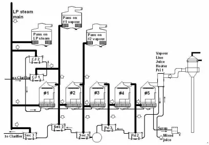
(34) 15 Chapter 1 Introduction •. Vapour bleeding creates large instabilities in the operation of the evaporator set and complicated control strategies are required to overcome this.. For the reasons stated above, the most common option employed in Australian factories is the use of vapour bleeding from the evaporator station. The use of vapour bleed systems has consequences for the evaporator station in that it is desirable to produce hotter vapours. Figure 1.9, from Wright (2000), shows a generalised evaporator/heater/vacuum pan vapour system for improved LP steam economy. Figure 1.9 shO\vs the use of vapour from the first effect (vapour one) being used for clarified and secondary juice heating and for use on the pan stage. Vapour from the second effect (vapour two) is used for secondary juice heating and for use on the pan stage. Vapour from the third effect (vapour three) and vapour four is used for primary juice heating whilst the vapour from the fifth and final effect is passed into the condenser. The limitations on the system are that the final. effect vapour pressure must be maximised and the LP steam supply to the first effect must be minimised, in order to obtain the optimum LP steam consumption. In this case the vessels are required to operate lNith higher HTC and lower effective temperature difference than would normally be experienced in factory operations.. These petfonnance indicators are discussed later in. section 1.3.3.. LP steam main. D. V'lfI O'" Ull e J llice He ater Pri 1. CJ 2. Sec~ + -. 10 Clarifi er S e c 3. Flgure 1.9. ,;. ,, '. S rll' Pri 2. Mi xe. jllice. Generalised evaporator/heater/vacuum pan vapour system for improved LP steam economy, Wright (2000).
(35) 16 Chapter 1 Introduction. 1.3. The Roberts vessel. 1.3.1. The basic design. Wright (1983) states that in Australian practice the evaporator vessels are of mild steel construction and use 18 gauge stainless steel (grade 304) tubes, from 1.6 m to 2.5 m in length, and 38 mm to 54 mm outside diameter. This is supported by the data seen in Bureau of Sugar Experiment Stations (BSES) (1992). The data published in this reference is a comprehensive listing of the evaporating plant found in all Australian raw sugar factories . An analysis of this data reveals that the most common tube size is 44.45 mm outside diameter (OD), with 63% of the total number of vessels in the industry having tubes of this diameter. Of the vessels with 44.45 mm OD tubes, almost 84% were made from stainless steel. Of all the vessels with 44.45 mm OD, stainless steel tubes, 48% of vessels contained tubes with a wall thickness of approximately 1.2 mm and had an average tube length of approximately 1.98 m. The shortest tube length was 1.53 m and the longest tube length was 2.70 m. This source of data is still considered to be the most reliable at present. The equipment found in factories is not expected to have changed substantially during the time since 1991.. 1.3.2. Vapour side operation. While there have been, and still are, many variants of the Roberts vessel, the operating principles have remained virtually unchanged. LP steam or vapour from the previous effect is fed into the calandria, through one or two inlet pipes, and condenses on the outside of the tubes. The condensate is removed from the bottom of the calandria and is usually pumped to a common condensate tank. The location of the condensate outlet varies depending upon the design and in some cases there may be more than one outlet point. Small amounts of air and other non-condensable gases are always present in the flow on the vapour side of the calandria. These gases are removed through vent pipes located within the array of calandria tubes. The location ofthe non-condensable gas vents varies significantly between designs. Gaps between the calandria tubes, called steam lanes, and baffle plates are often incorporated into the calandria design.. These steam lanes and baffles assist in the. dispersion of vapour around the calandria. The purpose of the steam lanes is to provide a path of lesser resistance for the vapour flow to those areas that may otherwise receive little flow. Baffles are used to divert the vapour flow to different areas around the calandria and towards the non-condensable gas take off points. Figure 1.10a, from Peacock (1999),.
(36) 17 Chapter 1 Introduction shows a branch type steam lane configuration installed in one of the Roberts vessels at the Proserpine Mill. In this design the vapour flow is predominantly down the lane in the middle of the vessel and branches out towards the exterior of the vessel. This type of vapour distribution system has no obvious point at which the non-condensable gasses will accumulate. Consequently the gas is removed from points throughout the calandria. Steam inlet. (b). (a) Figure 1.10. Steam lane and baffle design in Roberts evaporator vessels, Peacock (1999). Baffles have also been used to provide a more defined path for the vapour flow through the calandria. Figure 1.11, from Peacock (1999), shows two baffle designs. The zigzag baffle configuration has a higher pressure drop due to the sudden changes in direction but the helical baffle configuration has a longer path to travel.. Zig-zag baffling. Figure 1.11. Helical baffling. Types of baffles in Roberts evaporator vessels, Peacock (1999).
(37) 18. Chapter 1 Introduction Barnes and steam lanes can both be used on the same vessel in order to combine the improvements of both concepts. Figure 1. lOb shows one calandria design incorporating steam lanes and barnes. Although the vapour flow path shown in Figure 1. lOb is not as well defined as that in Figure 1.11 , the non-condensable gasses are tapped off from a single point. Another method of obtaining a more uniform vapour distribution within the calandria is to vary the tube layout. Tubes spacings predominantly have a rhombic (symmetrical) layout comprising of two equilateral triangles having 60° angles between sides. Tromp (1966) discusses a large variety of different tube layout designs and the effect on vapour flow around the outside of the tubes. Figure 1.12, from Tromp (1966), shows varying pitch tube spacing. In this configuration the portion of the tube bank closest to the vapour entry, approximately two thirds of the total tube-plate area, has a pitch that is 15% larger than the remainder. This encourages the vapour to evenly distribute throughout the calandria by providing a large area of lower resistance to the flow. The vapour then passes over the remainder of the tubes that have a smaller pitch. Figure 1.12 also shows a vessel with a central downtake on the juice side. Downtakes will be discussed in further detail later.. Figure 1.12. Variable tube pitch calandria, Tromp (1966). The vapour inlet system can also take the form of a belt around the outside of the vessel with a large number of smaller inlets into the calandria. Figure 1.13, from Peacock (1999), shows the vapour flow path around the belt. In this configuration the vapour does not enter.
(38) 19 Chapter 1 Introduction the calandria directly from the inlet pipe. Instead it is first passed through an annular space, or belt, around the outside of the vessel. The belt has the purpose of evenly distributing the vapour around all of the inlets into the cal andria. The vapour flow is predominantly radial in this case and has the advantage of a defined flow path, and therefore a defined tapping point, for the non-condensable gases. Non-condensable gases and condensate are removed from the centre of the vessel. This configuration can be used without the aid of steam lanes for flow distribution, but often steam lanes are included to ensure even vapour distribution.. Figure 1.13. 1.3.3. A circumferential belt producing radial vapour flow, Peacock (1999). Juice side operation. The basis of operation for the Roberts vessel is to feed juice into the space under the calandria of the vessel, usually from three or four points, and to withdraw juice through an outlet usually located close to the centre of the vessel. Some vessels employ baffles and other such devices to avoid short-circuiting but most will not.. The juice is drawn up. through the heating tubes once boiling is initiated. The vapour fraction increases towards the top of the tube and forms a small layer of 'froth ' above the top tube-plate. This mixture of juice and vapour above the top tube-plate is usually in the order of 150mm high. The static juice level within an evaporator is typically within the range of 30% to 60% of the tube height..
(39) 20 Chapter 1 Introduction The vapour released from the boiling liquid travels up from the calandria and into the headspace of the vessel. At the top of the vessel are entrainment arrestors, usually of the louvre type, to prevent the carry-over of liquid droplets into the calandria of the next evaporation stage. Since the detailed operation of the entrainment arrestors is outside the scope of this investigation, Wright (1988) and Henderson et al. (1981) should be referred to for further discussion on the topic. Evaporator operators will typically use the height of fluid above the top tube-plate as a means of controlling the operation of the vessel. Watson (1987) suggests that theoretically, the height of fluid above the top tube-plate should be minimised so as to reduce the static head above the boiling tube. However, the top tube-plate should not be allowed to dry out, as caramelisation of the sugar solution will occur.. This concept is supported by. experiments carried out by Guo et al. (1983) on a three-tube evaporator test rig. The test rig included an external leg to allow juice to return from above the top tube-plate to the space below the calandria. The downtake also included a valve so that the flow could be restricted and the static fluid height above the top tube-plate could be varied. It was found that the greatest HTC was achieved when the boiling juice was just wetting the top surface of the tube-plate. The test rig was operating under ideal conditions and the test results would suggest that the evaporator operators are incorrect in maintaining a static fluid height of approximately 150mm above the top tube-plate. However, less than perfect conditions and instabilities within the factory would account for the need to increase the height of the fluid above the top tube-plate when operating a full-scale vessel under factory processing conditions. Watson (1987) states that industry vessels generally do not have any means of returning the juice to below the calandria and it is assumed that those tubes which are boiling less intensely than average, act as downcomers. Watson (1987) also states that this effect could indeed be cyclic and cause instabilities in the fluid layer above the top tube-plate. Tubes could be boiling rapidly at one point in time and fluid could be flowing up the tube, while a short time later (perhaps a few seconds only), the boiling could have subsided and the tube could be acting as a downtake . No reference material has been located at this point in time to support or disprove this hypothesis. However, observations of the boiling surface in factory evaporators indicate that cyclic boiling behaviour, with regions changing from intense boiling to induced flow, is common. This may explain why factory vessels are operated at a static fluid level that is slightly greater than that found by Guo et al. (1983) in their test rig experiments..
(40) 21 Chapter 1 Introduction Quinan et al. (1985) discussed the design of a 51 OOm 2 evaporator installed at the Fairymead Mill during the 1984 crushing season. The calandria layout for this vessel contained many steam lanes and the multiple downtake locations within the tube layout. Watson (1987) investigated the effect of downtakes for reducing the fluid head above the tubes . Watson (1986a) further discussed the performance of the Fairymead evaporator from Quinan et al. (1985). A practical and well thought out approach by Watson (1986a) stated that a large number of smaller downtakes were thought to reduce the liquid level more effectively than a single central downtake, due to the very large diameter of the vessel. Watson (1986a) also highlighted that multiple downtakes have the added advantage of replacing the mechanical stays used to hold the top and bottom tube-plates. Watson (1986a) quantified the effect of the downtakes on reducing the head in the Fairymead evaporator, by measuring the head of fluid above the top tube-plate with a differential pressure level transmitter. The testing of operating scenarios, with and without downtakes was achieved by blocking the downtakes with plumbers ' expandable plugs, installed during a scheduled maintenance stop. The results of the tests took the form of a plot of head above the calandria versus level of juice in the tubes . Figure 1.14 from Watson (1986a) shows that there is a noticeable difference in the head with downtakes . The next logical step is to relate the effect of the downtakes to heat transfer performance by plotting the HTC for the two cases. Figure 1.15, from Watson (1986a), shows that the HTC with downtakes was approximately 250 W·m·2. K'1 higher than the corresponding HTC without downtakes, at the peak value. It should be noted that there is a lot of scatter in the data and Watson (1986a) makes no mention of accuracy in his discussion..
(41) 22 Chapter 1 Introduction 1500. WITH oa.H::CH:RS. -0-. .'. >lITl-OJT ~. ···X···. H. E. i/. A i). &, x~. 0 OOJ. F. 9. J. ;/if. U. If. I C E. x. ". x.''. ,e. 0. 0. 0 0. 0. 0 0. l<. v. 0. E. *. x x x,,'. 200. A L A N D R. ~. %. 0. c. 8. 0. """. 0. 0. 00. x. }:x. -.00. A B. fI0. 0. I,';. .,.x!~. 100. I. 0. 0. x. Xx. A. 0. $0. 0. 0. 2Il. 0. tI. 0 0. 0. 8' 0. 0. 80 0. 8. a LEVEL. Figure 1.14. ex. JUICE IN TUl£S. %. Plot of juice head above the calandria versus level of juice Watson (1986a). -. WITH. IJOI..NCa'ERS. Cll. 2. W(m K). 3000. o. H. o. T 2000. C l00e. 0. 2. W(m K). 3000 H. x~. x x )(. T. I. 2000. C. x )(. x l00e. 0 0. 10 L£VEL OF JUI CE IN 11JOCS. Figure 1.15. %. Plot ofHTC with and without downtakes, Watson (1986a). In. the tubes,.
(42) 23 Chapter 1 Introduction Those parts of the vessel that come into contact with the boiling juice tend to form a scale, particularly on the inside of the heating tubes. This scale acts as an insulator and therefore decreases the heat transfer performance of the evaporators over time. Various processes, usually involving the boiling of caustic soda or other such chemicals, remove scale periodically. Significant amounts of work in the area of scale removal and prevention have been done and there is a large amount of literature present. Doherty (2000) and Ivin and McGrath (1990) discuss the removal of evaporator scale using chemical cleaning processes. Crees (1983) and Abernethy et al. (1991) discuss the use of scale inhibitors.. These. references should be sought for fwther detail on evaporator scale. The insulating properties of scale must be taken into account conducting factory experiments. The scale formation process and its removal are outside the scope of this investigation.. 1.4. Evaporator performance. An overall HTC (U ) is used to quantify the heat transfer performance of evaporators. It is. found by measuring the overall heat flow through the calandria (Q) and averaging it over the entire HSA of the vessel (A) multiplied by the effective temperature difference between the hot and cold fluids (/:;T ), as per equation ( 1.1 ).. U =~ A/:;T. (1.1 ). Table 1.1, from Watson (1986), shows typical HTC values for each effect in an evaporator set. This method does not make any allowance for localised areas of high or low heat transfer, nor does it allow for the changes in heat transfer over the length ofthe tube . Table 1.1 Typical values of HTC for different effects, Watson (1986) Effect No. 1 2. 3 4 5. TypicalHTC (W·rn·l ·K') 2960 2470 2090 1550 610. The head of juice within the tube and the different boiling regimes experienced within the tube are expected to cause significant variation in HTC along the length of the tube. This method also assumes even LP steam or vapour distribution throughout the calandria. In.
(43) 24 Chapter 1 Introduction practice poor design of steam lanes and non-condensable gas removal systems (as discussed previously) will cause uneven heat transfer in different sections of the calandria Whilst this method is considered adequate for performance evaluation for factory type operation, it is considered inadequate for an in depth study such as the development of a CFD model and understanding of the flow regimes within the tube. The total heat flow through the calandria (Q) used in equation ( 1.1 ) must take into account any sensible heating of juice prior to the commencement of boiling and also any flashing of vapour from the juice at the inlet of the vessel. Appendix A to Broadfoot and Dunn (2001) details how these effects are accounted for in the calculations. The effective temperature difference (Ll.T) used in equation ( 1.1 ) is the difference between the saturation temperature of the LP steam or vapour in the calandria and the average temperature of the boiling juice. The saturation temperature of the calandria side is used regardless of the presence of superheat, as in the first effect. As water is evaporated from the boiling juice, the boiling point temperature is elevated above that for pure water at the same pressure. The boiling point elevation temperature (BPET) is described as the actual temperature of the boiling juice less the saturation temperature of water vapour at the headspace pressure. Batterham et al. (1973) published equations ( 1.2) to ( 1.5) below. First evaluating BPET at atmospheric pressure (T,")' where ff; and ~ are the sucrose to water and impurities to water ratios respectively:. . S J T = 2.442 - - 0.757 + 3.333 ' w W. (1.2 ). Where DS is the dry substance and P is the purity, it can be noted that:. S W. J W. =. DS. *. P. (lOO - DS) 100 DS • (lOO - P) (lOO - DS) 100. (1.3 ). (1.4 ).
Figure


+7

Related documents
The analysis is done on collector performance parameter with respect to absorber plate temperature, Air outlet temperature, Fin temperature, and for 0.03m 3 kg/s mass flow rate of
The effect of inlet heat transfer fluid temperature (Steffan number), mass flow rate and phase change temperature on the thermal performance of capsules of different radii have
c p : specific heat capacity (kJ/kg K − 1 ); E D : exergy destruction rate (kW); E in : input exergy (kW); h: specific enthalpy (kJ/kg); m: mass flow rate (kg/s); P: pressure (kPa);
Mass flow rate: 2 :5 kg/s Impeller tip speed: 475 m/s Mechanical efficiency: 96% Absolute air velocity at diffuser exit: 90 m/s Compressor isentropic efficiency: 84% Absolute
For the calculated Maximum Mass Flow Rate of 0.0703 kg/s, the Delta Pressure (Inlet Pressure – Outlet Pressure) was calculated for different converging and diverging angles..
Mass flow rate: 2 :5 kg/s Impeller tip speed: 475 m/s Mechanical efficiency: 96% Absolute air velocity at diffuser exit: 90 m/s Compressor isentropic efficiency: 84% Absolute
SHELL AND TUBE HEAT EXCHANGER(KERN'S METHOD) HOT FLUID-toluene SPECIFIC HEAT,J/KGK,CP: VISCOSITY,µ DENSITY ,Kg/m3,ρ; THERMAL CONDUCTIVITY,w/m2 k,K: MASS FLOW RATE Kg/s.
Thus, a low heat transfer fluid flow rate of 2 L/min (0.033 kg/s) produced the best thermal energy recovery process from the
