Development of a more energy efficient Roberts evaporator based on CFD modelling

Full text

(1)ResearchOnline@JCU. This file is part of the following reference:. Pennisi, Steve (2004) Development of a more energy efficient Roberts evaporator based on CFD modelling. PhD thesis, James Cook University.. Access to this file is available from:. http://eprints.jcu.edu.au/24949/ If you believe that this work constitutes a copyright infringement, please contact [email protected] and quote http://eprints.jcu.edu.au/24949/.

(2) 58 Chapter 4 Numerical modelling. 4.. Numerical modelling. 4.1. Introduction. The physical processes occurring inside an evaporator vessel are extremely complex when considered in their entirety. However, the physics associated with different parts of the process can be treated separately and some simplifying assumptions applied to build an overall descriptive model.. Since this investigation was the ftrst attempt to model an. evaporator vessel in its entirety, a number of simplifying assumptions have been applied to build a working model. Each assumption is justified in its use because the effect on the accuracy of the CFD model predictions is less than errors associated with the experimental data. Numerical modelling of the steady state operation for two different evaporator vessels was carried out in this study. This chapter outlines the equations governing the numerical model. As the physical processes occurring inside an evaporator vessel are extremely complex, the evaporator will be divided into different sections, and simplifications to the model made based on the dominant physical process occurring within each section. Two evaporator vessels being studied are the Proserpine #4 and Farleigh #2 vessels. Initially the Proserpine #4 and the Farleigh #2 geometries were modelled so that direct comparisons could be made with factory data. Once the accuracy of the model predictions had been conftrmed, the model was used to investigate possible improvements in performance. Initially a retro-ftt modification to the Farleigh #2 geometry was considered where a majority of the vessel remained unchanged except the juice inlet and outlet and downtakes were included in the calandria. Finally, a totally new design of evaporator geometry was considered. The concept involves a number of smaller calandrias operating in series and is referred to herein as the linear evaporator design. In total, four different evaporator geometries were considered for the modelling phase of this investigation.. 4.2. The software package. The software package used to solve the equations for this investigation was CFX version 5.5.. CFX contains standard options for most of the physics modelled as part of this. investigation but some user deftned sub-routines were required. This input me allows for the physics used during this investigation to be reproduced in CFX..

(3) 59. Chapter 4 Numerical modelling Appendix B contains an example of one of the input files used to model the Proserpine #4 vessel. It includes all of the details used in creating the CFD model used for this investigation. Included with this thesis is a Compact Disk (CD) containing the CFX input files used in this investigation. The inclusion of the input files to this thesis allows for the work to be reproduced by another researcher. This chapter provides details and explanation of the most significant portions of the CFD model used for this investigation. It includes details of all of the standard features employed and the user defined sub-routines added to the model.. 4.3. Model description. Geometrical symmetry, and hence the assumption of flow symmetry, was used to reduce the size of the computational mesh required. This was necessary since the size of the computational mesh was found to be the single largest contributor to the usage of computer memory which was insufficient to model the entire geometry of the vessel. Since there are a large number of symmetric boundaries inside the vessel that would obstruct the flow, it was assumed that asymmetric flows would be discouraged from developing and dominating the flow field. Details of the four cases considered are as follows : •. The geometry of the Proserpine #4 vessel displays one-quarter symmetry with four juice inlets and one central juice outlet. A single juice inlet and one-quarter of the outlet was modelled with two planes of symmetry;. •. The FarJeigh #2 vessel displays no actual symmetry since it has a single juice inlet and two different sized juice outlets. However, the difference in outlet size was neglected and it was assumed that the geometry of the vessel displayed one-half symmetry. Half of the inlet and one of the outlets were modelled with one plane of symmetry;. •. The geometry of the modifications to the FarJeigh #2 vessel displayed one-eighth symmetry with a single circumferential juice inlet and a single central juice outlet. One-eighth of the inlet and the outlet were modelled with two planes of symmetry; and. •. The linear evaporator was assumed to be 2-D and was modelled accordingly..

(4) 60 Chapter 4 Numerical modelling When the geometric symmetry of the vessels was considered it was recognised that geometric symmetry does not guarantee flow symmetry.. The errors resulting from. artificially induced flow symmetry are minimal in this case, because the boiling action inside the calandria is the dominant force driving the juice flow . It was assumed that the juice flowing up the heating tubes and down the downtakes would quickly dominate any juice flow pattern entering from the inlet. The factory experiments showed large amounts of juice recirculating around inside the vessels and this supports the justification for making this assumption. In all cases modelled, the steam distribution within the calandria was assumed to be uniform. A uniform heat source was applied everywhere within the calandria section. In the absence of any data in the literature to provide guidelines on steam distribution, the uniform heat source assumption is the normal assumption used for modelling heat exchangers in other industries. Each evaporator vessel was divided into three sections, one above the calandria, the calandria itself, and one below the calandria with all the juice inlets and outlets. Due to the complexity of the cal andria, it is not possible to model all the tubes. A lumped parameter approach is taken whereby the boiling/heat transfer and fluid flow in the pipes are each represented by a single heat flux and pressure drop relationship respectively. The two sections are then linked through boundary conditions that specify the interaction between the sections. In contrast, the first two sections can be modeled directly through solving the Navier-Stokes and heat equations with appropriate turbulence models and physical data correlating juice temperature and brix.. 4.4. Governing equations. For this particular case the three conservation equations of interest are the mass, momentum and energy equations defmed in terms of the volume fractions (aJ and a g ) as follows: The continuity equation for the liquid phase:. (4.1 ).

(5) 61 Chapter 4 Numerical modelling The continuity equation for the vapour phase:. (4.2 ). The momentum equations for the liquid phase:. (4.3 ). The momentum equations for the vapour phase:. (4.4 ). The energy equation for the liquid phase :. aa,p,h, at. (4.5 ). The energy equation for the vapour phase:. ( 4.6). The equation for the transport of sugar:. ( 4.7). The energy equation as shown in equations ( 4.5) and ( 4.6) has neglected the rate of work done by pressure forces and viscous forces . As velocities gradients are small except at the inlet or outlet regions and the viscosity is low for the sugar solutions, the contribution is small relative to the enthalpy of the fluid, and as such can be neglected. Work done by the pressure force is converted into kinetic energy with very little dissipation and hence does not contribute significantly to increasing the heat balance of the fluid. The rate of work done by gravitational forces is accounted through the additional source term. The region above and below the calandria is assumed to be liquid only and the liquid phase equations are solved in these regions..

(6) 62 Chapter 4 Numerical modelling For the cal andria, rather than solving the multi-phase equations detailed above, a lumped parameter model simplified the equations through the pressure term. The pressure drop inside the calandria section was separated into the three directional components, (see section 4.8.2) such that SMx. =:. and SMz. =:. as detailed in equations (4.8) and SMY. =:. as detailed in equation ( 4.9). This is a reasonable assumption since the vertical orientation of the heating tubes inside the actual vessel will prevent any fluid flow in the horizontal plane and the resulting fluid flow in the vertical direction is a simple flow through a smooth pipe. Details of terms used in these equations are described in more detail in section 4.7.2.. 4.5. Fluid properties. Fluid properties of the liquid and gas phases are required for the numerical solution of the model. The important properties are specific heat capacity, density, viscosity, boiling point elevation temperature and thermal conductivity. These properties have been correlated as functions of the fluid temperature and sugar concentration, and summarized in Appendix C. The properties of the gas phase have been assumed to be constant as the boiling takes place at a constant temperature. The gas phase properties are obtained from steam tables based on the headspace pressure measured in the vessel.. 4.5.1. Fluid temperature. The software package used assumes that the fluid is compressible if it is a function of temperature and automatically invokes the total energy model for solving the energy balance. The total energy model is computationally expensive and not required, as the density does not change significantly with temperature. To enable the program to continue to use the thermal energy model where incompressible flow is assumed, a constant temperature was substituted into the expression for liquid density. This constant temperature was set to be equal to the juice temperature at the inlet to the vessel. As shown in Chapter 5, the change in temperature in the vessel is quite small and this constraint should not affect the calculations and the conclusions significantly.. 4.5.2. Sugar concentration. The transport equation for the sugar concentration in the evaporator requires the diffusion coefficient of sugar in water. The kinematic viscosity of sugar varies from O.9xlO·6 m 2·s·1 at. o wt% sugar to. 1.2xlO·6 m2·s·1 at 22 wt% sugar to 3.7xlO·6 m 2·s·1 at 40 wt% sugar. The. Prandtl number (ratio of thermal diffusivity to kinematic viscosity) for boiling water is approximately 1.7 at atmospheric pressure and increases with decreasing pressure. For low.

(7) 63 Chapter 4 Numerical modelling sugar concentrations, the increase in liquid viscosity with increasing sugar concentration compensates against the increase in Prandtl number due to decreasing pressure.. The. maximum sugar concentration at the outlet is 65% where the Prandtl number is approximately 3.5 times the corresponding Prandtl number for water.. Based on the. properties of the sugar solution, the thermal diffusivity of the solution is taken to be approximately that of the kinematic viscosity as the data for kinematic viscosity is available but not that of thermal diffusivity.. 4.6. Boundary conditions. The boundary conditions are U I = 0,. ~~. = 0 for all the solid boundaries. The inlet. boundary conditions were based on the experimental values obtained from the factory vessels (see Table 3.11 and Table 3.12). Although the juice flowing into the inlet of the vessel has a small amount (approximately 5%) of vapour mixed in with the liquid, this amount is small and has been neglected. Table 4.1 and Table 4.2 summarises the boundary conditions applied to the inlet for the four cases modelled on the Proserpine #4 vessel and the six cases modelled on the Farleigh #2 vessel. Table 4. 1 Summary of the inlet boundary conditions for the CFD model of the Proserpine #4 vessel Test DO. Juice mass flow rate at inlet (m'·h·') Juice temperature at inlet ('C) Juice brix at inlet (%-wt). 1 258.2 87.8 35.6. 2 267.7 88.9 36.3. 4 273 .1 81.3 38 .1. 3 272. 1 81.3 37.7. Table 4.2 Summary of the inlet boundary conditions for the CFD model of the Farleigh #2 vessel Test no. Juice flow rate at inlet (m' ·h·' ) Juice temperature at inlet ('C) Juice brix at inlet (%-wt). 1 365.3 100.8 22.5. 2 315.3 100.9 21.7. 3 262.8 100.4 23.9. 4 277.7. 5 344.9. 99.8 22.7. 95.2 22.1. 6 341.0 101.0 22.4. The outlet boundary condition was P = 0 Pa. Applying a zero pressure at the outlet allows the pressure at the inlet and everywhere else in the fluid domain to be calculated relative to the outlet.. This process was adopted to avoid numerical problems with large absolute. values of pressure and because the pressure drop from inlet to outlet is the value of interest and is small in magnitude. If required, the absolute magnitude of the pressure at inlet and.

(8) 64 Chapter 4 Numerical modelling outlet can be calculated by adding the absolute pressure measured in the headspace of the vessel. The free surface of the fluid above the calandria was modelled as a rigid lid to the fluid TIlls surface was assigned a free slip boundary condition to allow lateral. domain.. movement of the fluid without pressure drop. The height of the free surface above the top of the calandria was set according to the measurements of free surface height taken as part of the factory experiments.. 4.7. Geometrical considerations. Geometrical details incorporated into the Proserpine #4 and Farleigh #2 models are detailed as follows: •. The Proserpine #4 vessel was modelled with one-quarter symmetry and symmetry planes at the boundary of the cut. The vessel includes a deflector plate placed immediately above the vertical inlet pipe and this was modeled as a rigid thin surface. The no-slip wall boundary conditions for velocity were applied to this surface. A single juice inlet and one quarter of the outlet was modeled with two planes of symmetry.. •. The Farleigh #2 vessel displays one-half symmetry with two juice outlets and a single manifold type juice inlet. A single juice outlet and half of the juice inlet manifold were modelled with one plane of symmetry the boundary of the cut.. 4.7.1. The calandria. The extremely large number of heating tubes in the calandria section made it impractical to model each tube individually. In order to simplify the modeling, the tubes were lumped into a single pressure drop . The physical orientation of the vertical heating tubes restricts the fluid flow to the vertical direction only. The calandria region operates to transfer heat from the steam side to the juice and effects boiling. The generation of vapour results in a two-phase mixture that separates further up the tube . The boiling provides a buoyancy force and this is modeled as a series of momentum sources.. The flow in the tube is. assumed to be transitional and a correlation based on the Colebrook equation was used. This new correlation fitted the Colebrook equation in the region of Re to 10000 (the Re of the problem varied between 100 and 7000) and was easier to estimate the friction factor than the Colebrook equation itself (Figure 4.1)..

(9) 65. Chapter 4 Numerical modelling The Colebrook equation was used for this investigation because of its simplicity and it can be easily incorporated into the lumped parameter model. A two-phase equation such as the Lockhart-Martinelli is more accurate but requires inputs that are not specifically calculated by the lumped parameter model. In order to set up a differential equation for the vapour and liquid fractions, the individual heating tubes would have to be modelled. This was not possible during this investigation.. 4.7.2. Flow constraint. The pressure drop is constrained to ensure that the fluid flow is essentially in the vertical direction, in accordance with the flow in the tubes. The larger diameter downtakes were modelled separately, but the heating tubes were modeled as a single entity due to the large number of small diameter tubes. A series of momentum sources, through a pressure drop relationship, were used to describe the flow inside the heating tubes. The basis for this approach is that the tubes direct the liquid flow upwards inside the heating tubes and down into the downtakes.. The pressure losses associated with the liquid flow and vapour. generation is essentially in the vertical direction as the flow is constrained. To constrain the flow, a pressure drop relationship was used to limit the horizontal flows . A pressure term in this case merely changes the flow and does not add to the energy balance. The default geometry of the vessels defined by CFX oriented that the y-axis as vertical. In this work the pressure drop in the two horizontal directions (x and z) were modelled as a momentum source, according to:. op Ox. =. - 50.0pt ~~' + v' + w'~ (4.8 ). The momentum sources detailed in equation ( 4.8 ) were defmed in a form where the magnitude of the momentum source would always act in the opposite direction to the fluid flow. The magnitude of the momentum source was also allowed to change according to the magnitude ofthe velocity vector. For example, a large momentum source would be applied to a node with a large velocity component in the horizontal plane and the magnitude of this momentum source would reduce as the flow approached the vertical orientation. This was found to have a significant influence on the time required for convergence.. Simply.

(10) 66. Chapter 4 Numerical modelling applying a large momentum source m the horizontal plane all of the time required significantly larger simulation times. The pressure drop in the vertical direction (y), assuming the fluid flow to be laminar and single phase, was approximated by:. op = 0;. _{I ~l PmJ. (4.9 ). A, 2d. The A, term is used in equation ( 4.9 ) to account for the tube area relative to the calandria section area. The friction factor (f) as applied in equation (4.9) is a modified version of the Colebrook equation. Since the flow in the calandria section of this vessel is predominantly in the laminar and transitional flow regions, an explicit form of the friction factor equation was used to avoid the iterative nature of the Colebrook. Figure 4.1 shows a plot of the standard friction factor equations for laminar and turbulent flow and the modified equation applied in this case. The fmal form of the equation used is: 10. ~,. Le.mine.r regi c.n. ,,. ~. Turbulent f"9gion. T ra nsiti onal regior. ,,. ---64lRe - - - -smocth pipe. ,, 0 .1. - - O.027+53.33/Re. ,. '~ ",. ---,,. ,,. ---- -- .-. ---. 0.0 1. 10. 100. 1000. Re. Figure 4.1 Plot of friction factor versus Reynolds Number. 100 0. 1000 00.

(11) 67 Chapter 4 Numerical modelling. f. =. 0.027 + 53.33 Re. (4.10 ). Figure 4.1 shows that the modified equation slightly under-estimates the friction factor at very low Reynolds Numbers and slightly over-estimates the friction factor at higher Reynolds Numbers in the turbulent region but allows for a smooth transition through the transitional region that the standard equations do not.. The largest Reynolds Number. experienced in the calandria region is approximately 7000. for which the friction factor from equation ( 4.10 ) agrees well with the Colebrook equation.. 4.7.3. The gaseous phase. The total two phase flow in the boiling region is the sum of the component flows such that W = Wg + W, . The volumetric rate of flow, represented by the symbol Y, is given as a total. Since Y. sum of the volumes Y = Yg + Y, .. = wp , substitute to get. w p. = W,p + w,p and take. ';; = X and ~ = (I - X ) . The average density then becomes: _I = _X + ", (I_-_ X...!..). Pm. Pg. P,. ( 4.11 ). where X is the mass fraction of vapour present. Similarly, the viscosities are assumed to be linearly summable. Although this assumption is an analogy, it provides a reasonable assumption of the average viscosity. The average viscosity then becomes:. -. I. Pm. X. =-. Pg. (I - X). + -'----'PI. (4.12 ). The calculation of Reynolds Number is perfonned using the averaged fluid properties such that:. (4.13 ). In the calculation of the flow inside the cal andria, the liquid and gas phases were modelled as a single phase to simplify the calculations. In so doing, the slip velocity between the liquid and gas phases were assumed to be small. Terminal velocities of air bubbles in pure.

(12) 68 Chapter 4 Numerical modelling water varies from 0.2 to 0.4 ml s depending on the bubble size (0.001 to 0.04 m diameter), and hence the terminal Reynolds number, as discussed by Clift et al. (1978).. With the. addition of impurities, it has been found that the terminal velocities are reduced to around 0.2 ml s for the same bubble size range . The effect of relative viscosity has been discussed. by Clift et al. (1978) and is found to be small but the results have not been obtained for liquids of high viscosities. In the case of slug flow, the terminal velocity has been found to reduce inverse proportionally to the kinematic viscosity; hence a doubling of the kinematic viscosity will reduce the terminal velocity by half.. The case in the calandria will be. somewhere in between, with the walls of the calandria having a small effect on the bubbles, depending on size. A finite wall also reduces terminal velocity, the extent dependent on the bubble to heating tube diameter ratio. As the space above the calandria shows some degree of foaming, it is expected that the bubbles are not large. The impurities and viscosity of the juice will act to prevent coalescence of the bubbles formed due to boiling. As such the slip velocities between the liquid and gas phases will not be large, in this case, it should be less than 0.2 mIs, possibly much lower. However, there is a dearth of information regarding the bubble terminal rise velocity for juice and it is recommended that future work should include a study of the bubble terminal rise velocity. The results from the simulations show that the slip velocity of the liquid and gas phases, if included, will not dominate the flow. To a first order, the deletion of the slip velocity should not severely affect the results of the simulation, however, a more accurate model should include the effect of slip velocity. The assumption of zero slip velocity allowed the calculation of the average fluid properties in each controlled volume, since the liquid and gas were assumed to be flowing at the same velocity. As a result of this calculation the density of the fluid inside the calandria was reduced. The lighter fluid inside the calandria behaved more like the actual fluid where the bubbles would rise up through the liquid inside the heating tubes . For those cases where the calandria of the vessel was fitted with downtakes, these geometries were modelled specifically.. It was assumed that no juice heating occurred. inside the downtakes and therefore no vapour was produced. The walls of the downtakes were included as thin surfaces with free slip boundary conditions. Only the momentum source acting in the vertical direction, see equation ( 4.9 ), was applied to the fluid flowing inside the downtake. The fluid was allowed to flow laterally inside the down-take since this is what occurs in reality..

(13) 69 Chapter 4 Numerical modelling The juice flowing into the vessel through the inlet was modelled as liquid phase only. The quantity of vapour resulting from the juice flashing before entering the vessel was neglected. The quantity of flashing was calculated to be approximately 5% of the total mass flow rate of juice at the inlet and contains approximately 13% of the heat which is transferred through the calandria.. All of the juice inlet systems considered in this. investigation are fitted with distribution devices which spread the incoming liquid and vapour immediately before the flow enters the bulk of the liquid. These devices will spread the juice in all directions and reduce the effect that the vapour has on the flow field in the remainder of the vessel. Modelling of the vapour phase in the incoming juice will add significant complexity to the CFD model and will require significantly more computing resources than are currently available.. 4.8. Heat flow inside the calandria. The total thermal energy (Q), released by the condensing steam, neglecting thermal losses, was assumed to go into the latent heat of evaporation, producing vapour and sensible heating of the remaining liquid, due to the effect of boiling point elevation.. Q = Q, + Q,. ( 4,14 ). where: ( 4,15). Q, = m" Cp,(T, - T). ( 4,16). The two components of the heat flow (Q, & Q, ) were applied as a boundary condition and set as two separate source terms in the energy and the continuity equations. The source term in equation ( 4.5 ) was set such that S E. =. Q, . The amount of heat that flows into the. vapour during the evaporation process was accounted for in the mass source term in equation ( 4.1 ) such that S c = f- . To prevent evaporation from occurring before the juice. ". reached it boiling temperature, the source term was linked to the temperature of the fluid such that:.

(14) 70 Chapter 4 Numerical modelling. (4.17 ). Initially the total heat flow. (Q). was set to be equal to the experimentally measured value. for each test condition. This was required for comparison purposes since the heat flow determined the evaporation rate and therefore the sugar concentration. So it was necessary when comparing factory measurements with predictions to apply the same evaporation rate. After the initial model comparisons were completed. all of the test conditions were remodelled such that the total heat flow. (Q). was calculated. The total heat flow was. calculated according to the following equation. which was developed by Rohsenow (1952) and is detailed in Incropera and DeWitt (1996):. ( 4.18). The values of C,i and n as applied in equation ( 4.18) were set to typical values for water and stainless steel as displayed in a table taken from Incropera and De Witt (1996). The magnitude of these values were C'I. =. 0.013 and n = 1.0 accordingly.. Equation ( 4.18 ) was developed predominantly for water and considered a number of different surface types, of which included stainless steel as in this case. The form of the equation is considered suitable for application in this case because it takes into account the effect of varying fluid properties and varying surface-fluid interactions on heat transfer. The fluid properties of sugar solutions at lower concentrations are very similar to water. A similar study by Hong et al. (2004), published after the completion of this investigation, supports the justification for the use of equation ( 4.18). Hong et al. (2004) conducted a comprehensive experimental investigation into the effect of varying fluid properties on heat transfer and the data correlated well with an equation in the same form as equation ( 4.18 ). However, the influence of fluid properties was accounted for by modifying the value for C if as follows :. c _. 0.04. 'I -. 1 + (B!14.75)"". ( 4.19).

(15) 71. Chapter 4 Numerical modelling Where B is the concentration of sugar (%(w/w)), otherwise referred to as brix for the purposes of this investigation. Equation ( 4.19 ) was obtained experimentally using a linear regressIOn. Hong et al. (2004) reports errors of ± 10010 from the modified form of the equation and this is significantly more accurate than many other heat transfer equations. The success of Hong et al. (2004) suggests that the current equation may have the potential to be modified to take into account more of the physics and produce accurate heat transfer predictions. However, further investigation is required in order for this to be demonstrated. The effect of scale growth on the surfaces of the heating tubes has been neglected for this investigation. Equation ( 4.18 ) has the potential to take into account the effect of scale growth by changing the values of C st and n . However, successful validation the CFD model requires more accurate experimental data than is currently available.. 4.9. Fluid flow above the calandria. The fluid flow above the calandria was assumed to be all liquid phase with small buoyancy forces arising from the liquid density variation with sugar concentration. This is similar to the fluid flow below the calandria.. However, when applied to the region above the. calandria this assumption is far from reality.. The fluid above the calandria will have. significant variation in liquid mass fraction.. The fluid emerging from the top of the. calandria will have a liquid mass fraction less than 1, caused by the evaporation process inside the calandria. At the free surface of the fluid the vapour will disengage from the liquid phase and so leave the behind the liquid phase with a liquid mass fraction equal to 1. The variation of fluid quality with vertical height is likely to be highly non-linear. There is no information in the literature to describe this variation and the determination of such was considered to be outside the scope of the factory experiments conducted as part of this investigation. For these reasons the fluid quality in the region was set to be equal to 1 and the presence of the vapour phase was therefore neglected. The justification for making this assumption is that a fluid quality equal to 1 will produce the largest possible buoyancy forces trying to force any of the heavy juice above the calandria to flow back down the heating tubes or the small down-takes. This has been observed to occur in reality and although the absolute magnitude of the forces involved may be calculated incorrectly, the basis for the fluid behaviour remains correct..

(16) 72 Chapter 4 Numerical modelling. 4.10 Turbulence modelling The k - [; model was used in this simulation to model turbulence. The two equations for the turbulence kinetic energy (k) and the turbulence dissipation rate ([; )are as follows:. (4.20 ). (4.21 ). where p. is the turbulence production due to. VISCOUS. and buoyancy forces , which. IS. calculated as follows : (4.22 ). The values for the constants are C" U. £. ~. ~. 1.44, C el. ~. 1.92, C #. ~. 0.09,. Uk ~. 1.0 and. 1.3. The use of a turbulence model for modelling the turbulence present in a flow is. required to provide closure to the Reynolds averaged N-S equations. The k - [; turbulence model used in this numerical work is a second-order model wherein the stress-equations are included. A turbulent kinetic energy equation and a dissipation rate equation are solved to obtain the turbulent viscosity. The k - [; turbulence model here is a low Reynolds number form here following that of Jones and Launder (1972) where the model constants are standard and have not been adjusted.. Adjustment of the constant is not recommended. except when good quality experimental data is available for comparison and evaluation. A law of the wall is used to treat the inner region. The flow is not highly complex, except in the tubes in the calandria. Elsewhere, the flow generally follows a smooth path from inlet to outlet, possibly with substantial bypassing, to avoid the calandria region.. As such the k - [; model should provide a reasonable. estimation of the influence of turbulent dissipation, although it is generally more dissipative. The more complex turbulence models are able to better predict turbulence but are less stable. The model has restrictions in that it is a turbulent viscosity model assuming the Boussinesq approximation. A derivation of the k - [; model by the renormalisation approach show that.

(17) 73 Chapter 4 Numerical modelling the constant are not constants but there is no indication in the literature to suggest that this approach is any better for two-phase flow problems. For two phase flow problems, the energy spectrum has been shown to be quite different from single phase flow problems, particularly in the region where the buoyancy effects are significant. Liovic et aL (2003) using LES and Fulgosi et al. (2003) have shown that the enhanced energy decays according to the 8/3 power law seen in bubbly flow exist and confirms Lance and Bataille (1991) early experimental observation. Furthermore, the complete range of 5/3 to 8/3 energy decay power laws need to be predicted by a model in the bubbly region for the sub-inertial range. This cannot be predicted by any simple Class I or Class II (e.g. k - 5) turbulence model. The calandria region is expected to be in such a bubbly flow regime and the advection of vapour bubbles into the upper and lower regions of the evaporator is likely to produce complex turbulent flow interactions. Currently the LES model requires 32 computers approximately two weeks to generate a few seconds of results for evaluation Liovic et al. (2003); the extension to an evaporator simulation is not likely for a few decades. The use of the k -. 5. model is justified as it is a low Reynolds number turbulence model, is robust in. its application, does allow the prediction of laminarisation (the original topic of the paper on the model itself), and the computing power required for an accurate turbulence model for two-phase flow is yet to come.. 4.11. Convergence criteria. For both evaporators two convergence criteria were defined with the requirement that both must be satisfied before the simulation is complete. The root mean squared (RMS) residual errors for the momentum calculations in the three component directions, the additional variable calculations for sugar concentration and the energy calculations for heat flow had to be less than 1.0xlO·4. In this case taking all of the residuals throughout the domain,. squaring them, taking the mean and then taking the square root of the mean obtains the RMS residual error. A second convergence criterion was also established as the overall mass balance defmed as follows: (4.23 ). In most cases the overall mass balance was the last criterion to be met due to its relatively small magnitude. However, it was found to be necessary to ensure accurate calculation of.

(18) 74 Chapter 4 Numerical modelling the sugar concentration at the outlet. Simulations where the mass balance criterion was not used showed significant error in the predicted sugar concentration at the outlet, even though the residuals target was satisfied.. 4.12 Meshing of the geometry The geometry of the vessel was modelled with a finite volume approach, using an unstructured mesh.. Tetrahedral shaped mesh elements were used for a majority of the. volume, with pyramidal and orthogonal shaped mesh elements used for those regions inunediately adjacent to any external walls or internal walls with a no slip boundary condition applied. The different shaped objects at the wall were used to reduce the numerical diffusion problems commonly encountered with tetrahedral shaped mesh elements adj acent to walls. The number of orthogonal shaped mesh elements attached to any wall in all cases was five layers. The height of each layer varied slightly between cases depending on the estimated local velocity gradients that were checked after the first model was run. The size of the mesh was found to be the single largest contributing factor to the usage of computer memory. As mentioned previously in this chapter, maximum advantage was taken of the symmetry of the vessels, in an attempt to reduce the size of the computational mesh.. 4.12.1 Mesh independence Before the majority of the modelling began a mesh independence test was conducted using the Proserpine #4 geometry. The one-quarter geometry model was created and all of the physics that were to be used in the final model were implemented. The only simplification applied to the physics was that 10% of the evaporation rate was applied instead of the full evaporation rate . The evaporation rate was reduced since it was found to be the one parameter that caused extended solution times. This was especially important in this case since the large mesh size being used increased solution times. All of the other physics associated with the model were included since it was believed that any further simplifications would prevent the mesh independence being an accurate representation of the model once it is applied in full . Four different mesh densities were applied to the geometry, detailed as follows: •. the "coarse" mesh contained 24832 nodes,.

(19) 75. Chapter 4 Numerical modelling •. the "medium" mesh contained 239963 nodes,. •. the "fine" mesh contained 324121 nodes, and. •. the "very fine" mesh contained 532488 nodes.. The "very fme" mesh was used as a comparison for the other mesh densities. The "very fine" mesh simulation required a second computer running in parallel.. The second. computer was only available for a short period of time and could not be used for all modelling completed as part ofthis investigation. The "fine" mesh density was used for all subsequent modelling. After the four simulations were completed the solution from the very fine mesh was compared with the solution from the coarse, medium and fine meshes. The predicted velocity and sugar concentration fields for the coarser meshes were interpolated onto the node locations of the fine mesh.. The difference between the predictions was then. calculated at each node location in the fine mesh. For each mesh comparison, the error was calculated with the L2 norm error according to:. error. =. (4.24 ). i =l. n. Where x can be substituted for any variable and n is the number of mesh nodes . The velocity and the sugar concentration variables were chosen as the two variables to use for comparison purposes. These variables were used since they were believed to be the two variables most likely to influence the predicted solution. The combined results of the mesh comparisons is displayed in Table 4.3 Mesh Course Medium Fine. Calculated errors from different mesh densities Num ber of nodes 24832 239963 3241 21. Velocity error (m/s) 0.357 0.037 0.026. Brix error ('10 ) 4.99xlO·' 5.l7xlO"' 3.17xlO""'. Figure 4.2 is a plot of the velocity errors on a logarithmic scale and Figure 4.3 is a plot of the brix errors on a logarithmic scale..

(20) 76 Chapter 4 Numerical modelling In (no. of nodes) -1. IP ~. -1 .5. 11. 11.5. ~. -2. 1-2.5. ~. y = -1.01x + 9.21 R' = 0.9997. .=. -3. 12. ~. -3.5. Ip. 12.5. ~. "+. -4. Figure 4.2 Plot of the velocity errors relative to the "very fine" mesh In ( no. of nodes) ·5. Ip ~ -5.5. "C' -6.5. ~. 11. ~. ~. y=-1 .04x + 528 R' = 0.9964. ~. .!!.. .=. 10.5. -7. -7.5. 11.5. 12. 12.5. ~. ~. -8.5. Figure 4.3 Plot of the brix errors relative to the "very fine" mesh. ~•. 1~.

(21) 77 Chapter 4 Numerical modelling The slope from Figure 4.2 and Figure 4.3 is approximately -1, indicating first order convergence. Hence, the error will decrease by half for every doubling of the mesh density. As all the simulations at different mesh densities do converge, stability is not a problem. The "fme mesh" is expected to provide an error of ± 2.6% relative to a mesh independent solution.. Although the qualitative results in the subsequent solutions have a ± 2.6%. average error, the simulation results are expected to be qualitatively correct as the simulation is stable.. 4.13 Summary of the numerical model The complicated physics that occurs inside an evaporator requITes some simplifying assumptions to be made so that a useful CFD model of the flow inside these vessels can be developed.. The mathematical representation of the vertical heating tubes inside the. calandria region have shown that it is possible to adequately account for the influence they have on the fluid flow in this calandria, without modelling each tube specifically. Significant complexity was avoided by employing an Eulerian-Eulerian approach to the multi-phase nature of the fluid. The entire fluid was treated as a liquid with variations in density. Assuming zero slip between liquid and vapour allows for the average density and the resulting buoyancy forces to be calculated. Modelling of the bubble dynamics was not possible in this investigation since the fluid was assumed to be single phase. Modelling of the gaseous phase was not possible given the resources available for this investigation. Mathematically modelling the heating tubes inside the calandria and taking advantage of symmetry were all steps taken to reduce the size of the computational mesh. In this study the available memory resources of the computer hardware were a limiting factor on the size of the computational mesh that could be used. In spite of efforts taken to reduce memory requirements, a mesh independence test showed that the model predictions are slightly mesh dependant. This must be taken into consideration when examining the results of model predictions produced as part of this study. However, the results are believed to be adequate enough to produce useful and realistic trends. A suitable equation to describe the heat transfer process from stainless steel heating tubes to sugar solutions does not exist in the literature. A standard equation for describing the heat transfer process from a stainless steel heating surface to pure water has been applied. However, the form of the equation does allow for adaptation with further research, since it is in a form where the empirical constants can be modified to suit sugar solutions..

(22) 78 Chapter 5 Model validation results. 5.. Model validation results. 5.1. Introduction. Validation of the CFD model predictions is necessary to provide a means of judging the model's ability to reproduce the actual fluid flow behaviour inside evaporator vessels. As simplifications to the process are required for modelling, validation provides confirmation that the physics of the fluid flow has been adequately represented.. If the model can. accurately represent the physics then it can be applied as an engineering design tool. Previous chapters of this thesis have described the factory data gathered and the equations used in the model.. This chapter will provide a comparison between the predictions. obtained from the model and the data gathered from the factory vessels. The result of this comparison will allow the accuracy ofthe CFD model developed to be quantified.. 5.2. Validation procedure. The factory experiments provide juice brix and temperature measurements at strategic points in the region below the calandria as well as the total heat flow through the calandria. The validation was performed in two steps; 1) validating the juice brix and temperature at strategic points, and 2) validating the heat flow through the calandria. For the first validation step, the heat flow through the calandria was applied as a boundary condition equal in magnitude to the value provided from the factory experiments. This procedure was performed as a means of simplifying the model. By fixing the heat flows through the calandria the calculations required for the overall heat balance on the vessel were simplified and the energy equations were de-coupled from the brix and temperature predictions. Equation ( 4.18 ) includes a number of terms that are a function of the juice brix and temperature and replacing this equation with a constant value provided faster convergence and ensured that the heat flow through the calandria was the same as the value provided by the factory experiments. For the second validation step, the heat flow through the calandria was calculated according to equation ( 4.18 ), with the initial guess for the solution being set to the fmal solution obtained from the first validation step..

(23) 79 Chapter 5 Model validation results. 5.3. Validating the juice brix and temperature distribution. The results from all of the four tests conducted on the Proserpine #4 vessel and the six tests conducted on the FarJeigh #2 vessel were used for validation. The complete data set has been given in Chapter 3 (Table 3.3 and Table 3.4); this chapter includes only the j uice brix and temperature data used for validation purposes. Table 5.1 and Table 5.2 show the comparisons between the measured and predicted juice temperature data from the Proserpine #4 and the FarJeigh #2 vessels respectively. The magnitude of the difference between the measured and the predicted juice temperatures is reported, along with the difference expressed as a percentage of the temperature difference between the steam and the juice at the time of testing.. The difference between the measured and predicted. temperature values was expressed as a percentage of the temperature difference because the absolute magnitude of the juice temperatures is significantly larger than the small differences in temperature required for adequate validation. The effective temperature difference also changes from one factory experiment to the next and allows for the changes in operating conditions to be accounted for. Table 5. 1 Measured and predicted juice temperature data from the Proserpine #4 vessel. I Test No. 1 Point A PointE Point C Test No. 2 Point A PointE Point C Test No. 3 Point A PointE Point C Test No. 4 Point A PointE Point C. Measured ('C). P r edicted ('C). D ifference ('C). Differ ence (%). 55.1 55 .0 57.0. 55 .8 55.8 55.9. +0.7 +0.8 -1.1. +2.2 +2.5 -3.5. 55.5 55 .1 57.3. 55.9 56.0 56.0. +0.4 +0.9 -1.3. + 1.2 +2.8 -4. 0. 57.6 56.0 58 .8. 57.7 58.0 58.0. +0.1 +2.0 -0.8. +0.4 +8.7 ·3.5. 58.0 57.3 58 .8. 58.0 58.2 58.3. -0.03 +0.9 -0.5. -0.1 +4.0 ·2.2.

(24) 80 Chapter 5 Model validation results Table 5.2 Measured and predicted juice temperature data from the Farleigh #2 vessel. I Test No. 1 Point A PointB Point C Test No. 2 Point A PointB Point C Test No. 3 Point A PointB Point C Test No. 4 Point A PointB Point C Test No. 5 Point A PointB Point C Test No. 6 Point A PointB Point C. Measured (' C). Predicted (0C). Difference (' C). Difference (%). 98 .4 97.3. 100.1 100.2. +1 .7 +2.9. +26.6 +45.3. nI.. nla. nI.. nla. 98 .5 97.2 95, 0. 100.1 100. 1 100,1. + 1.6 +2.9 +5.0. +24.6 +44,6 +76,9. 9 1. 9 91.3 90.2. 96.2 96.3 96.3. +4.3 +5.0 +6.1. +75.4 +87,7 + 107. 93.3 92,6 92.3. 95.4 95.5 95.5. +2.1 +2.9 +3.2. +32.8 +45.3 +50,0. 92.2 92.4 93. 1. 96.9 970 97.0. +4.7 +4.6 +3.9. +75.8 +74.2 +62.9. 95 ,2 94.0 94.7. 97.2 97.3 97.3. +2.0 +3.3 +2.6. +33,8 +55.9 +44. 1. The juice temperature predictions from the Proserpine #4 vessel show close agreement with the measured values, but the predictions from the Farleigh #2 vessel show significant variations in both absolute magnitude and in percentage terms. Some possible explanations for this difference are as follows : •. It is possible that the factory experiments were unable to measure the JUice. temperature to the level of accuracy required for very detailed comparisons, •. The model developed as part of this study is more suited for vessels operating with higher juice brix, and. •. The physical differences between the Proserpine #4 calandria and the Farleigh #2 calandria are causing the fluid to behave differently and this behaviour is not being captnred by the model predictions.. Table 5.3 and Table 5.4 show the comparisons between the measured and predicted juice brix data from the Proserpine #4 and the Farleigh #2 vessels respectively. The magnitude.

(25) 81 Chapter 5 Model validation results of the difference between the measured and predicted juice brix is reported, along with the difference expressed as a percentage of the juice brix change from inlet to outlet. These data were included because the change in juice brix from inlet to outlet can be quite small, particularly for early effect vessels such as the Farleigh #2.. Table 5,3 Measured and predicted juice brix data from the Proserpine #4 vessel Measured (%-wt) Test No.1 Point A Point B Point C Test No. 2 Point A Point B Point C Test No. 3 Point A Point B Point C Test No. 4 Point A Point B Point C. I. I Difference (%). Predicted (%-wt). Difference (0/0 -wt). 63.5 65.0 63.6. 61.4 61. 9 62.4. -2. 1 -3.1 -\.2. -7.7 -11 .4 -4.5. 64.4 65.7 64.5. 61.7 62.4 62.9. -2. 7 -3.3 -1.6. -9.8 -11.9 -5 .9. 68.5 72.9 67.1. 64.5 66.7 66.9. -4.0 -6.2 -0.2. -13.5 -20.9 -0.7. 68. 1 69.1 66.7. 64.2 66.2 66.6. -3.9 -2.9 -0.1. -13.5 -9.9 -0.4. Table 5.4 Measured and predicted juice brix data from the Farleigh #2 vessel Measured (% -wt) Test No. 1 Point A Point B point e Test No. 2 Point A Point B point e Test No. 3 Point A Point B point e Test No. 4 Point A Point B point e Test No. 5 Point A Point B. I. I Difference (%). Predicted (% -wt). Difference (0/0 -wt). 28.3 27.4. 25.9 26.0. -2.4 -1.4. -58.3 -33.6. nla. nla. nla. nla. 27.1 26.4. 25.2 25.2. -1.9 -\.2. -48.7. nla. 25.1. nla. nla. nla. 27.2 27.4 27.4. nla. nla. -\.3 -0.1. -32.2 -2.4. 26.5 26.7 26.8. nla. nI.. -0.8 +0.4. -18.0 +8.1. 25.5 25.7. -\.2. 28.7 27.5. nla 27.5 26.4. nla 26.9. I I. nla. -30.5. I I. nI. -29.0.

(26) 82 Chapter 5 Model validation results PointC Test No. 6 Point A Point E Point C. 26.0. I. nla 27.2 26.4. I. 25. 8. -0.2. -5.8. 25.8 26.1 26. 1. nla. nI.. -1.1 -0.3. -27.0 -6.. 5. The juice brix predictions for both the Proserpine #4 and the Farleigh #2 vessels show reasonable agreement with the corresponding measured values, except for the first two tests conducted on the Farleigh #2. This difference is likely caused by the location of the sampling points, as is discussed later.. 5.4. Discussion of the juice brix and temperature validation. The predicted juice brix distribution for the Proserpine #4 vessel shows reasonably close agreement with the measured data. The largest difference being - 20.9% for point B during test number 3. For all other points the difference between measured and predicted data is less than - 13.5%. It must be noted that only point B in test number 1 was located above the bottom tube-plate of the calandria i.e., inside the heating tubes. While the data from the Proserpine #4 vessel shows reasonable agreement between measured and predicted values, it can only be considered an indication of the flow in the region below the bottom tubeplate. The flow behaviour inside the calandria is likely to be significantly different due to the complexity of the physical processes occurring in this region. This is a significant limitation in these validation data due to the number of simplifying assumptions that have been made in order to model the calandria section. The predicted juice brix distribution for the Farleigh #2 vessel shows larger differences from the measured values, in particular tests number 1 and 2. However, the location of the sampling points for both of these tests is above the bottom tube-plate of the calandria. Due to the size ofthe sampling probe being only slightly smaller than the heating tube itself it is possible that the presence of the sampling probe in these locations has adversely affected the fluid flow. If this is the case then it is likely that the measured data will be significantly different to the predicted data. The remainder of the data from the Farleigh #2 vessel are located in the region below the calandria and show reasonable agreement between the measured and predicted values. Even though some of the differences are larger than those from the Proserpine #4 vessel the juice brix predictions in the region below the calandria are still considered acceptable..

(27) 83 Chapter 5 Model validation results The data shows that in almost all cases the juice brix is under predicted for both vessels, but the juice temperature is over predicted. This is a strange result since an under predicted juice brix would result in an under predicted boiling point elevation temperature. If this were the case then the juice temperature would also be under predicted. The cause of this difference is the magnitUde of the juice temperature at the inlet. This boundary condition was determined directly from the factory measurements. It is possible that this temperature was measured incorrectly during the experiments and the associated error has followed on to the model predictions. Since the variation in juice temperature any errors in the juice temperature boundary condition applied at the inlet will have a significant effect on the predicted juice temperature distribution throughout the vessel. The predicted juice brix and temperature data shows good agreement with the measured data in general terms and the observed trends have been predicted reasonably accurately. The range of processing conditions covered during the factory experiments was sufficient to cover a majority of the conditions normally experienced in an evaporator set with a large difference in the operating temperatures of the two vessels. The model applied to both vessels was exactly the same with no arbitrary constants or empirical values used in either case. This supports the accuracy of the predictions in general terms even though it must be recognised that some differences exist between the absolute magnitude of the juice brix and temperature predictions, when the heat flow through the calandria is applied as a boundary condition.. 5.5. Validating the heat flow predictions. The processing conditions experienced during factory testing were all applied as boundary conditions to the CFD model during the validation procedures for the juice brix and temperature.. When validating the heat flow predictions the boundary condition was. replaced by the expression detailed in equation ( 4. 18 ), and the measured heat flow was used for comparison purposes. For comparison purposes the values displayed as the heat required for evaporation from Table 3.5 and Table 3.6 have been used as the measured values. The magnitude of the difference between the measured and predicted values is expressed as a percentage of the measured value..

(28) 84 Chapter 5 Model validation results Table 5.5 Measured and predicted heat flow data from the Proserpine #4 vessel Test No. 1 Test No. 2 Test NO. 3 Test NO.4. Measured (MW) 73 .52 75.02 82.18 80.72. Predicted (MW) 64.90 65.30 49. 15 48 06. Difference (%) -11.7 -130 -40.2 -40.5. Table 5.6 Measured and predicted heat flow data from the Farleigh #2 vessel Test No. 1 Test No. 2 Test NO.3 Test No. 4 Test NO. 5 Test NO.6. Measured (MW) 30. 59 26.4 1 22. 12 26.07 30.12 29.93. Predicted (MW) 37.60 39.44 21. 89 31.53 33.14 29.15. Difference (%) +22.9 +49.3 -1. 0 +20.9 +10.0 -2.6. The results of comparison between the measured and the predicted heat flows show varying levels of success. The heat flows in the Proserpine #4 vessel is always under predicted, but is within acceptable limits for the frrst two tests . However, there is a predicted decrease in heat flow for the second two tests and this change is in the opposite direction to the measured data. When considering tests numbers 3 and 4 were conducted immediately after the evaporator was cleaned, the data would indicate that the effect of cleaning is not being captured. However, the same behaviour is not displayed in the FarJeigh #2 data. In this case the two tests conducted after the evaporator was cleaned (test numbers 5 and 6) show good agreement between the measured and the predicted heat flows. Also, the heat flow in the Farleigh #2 vessel is over predicted for the tests conducted before the evaporator was cleaned. This can be explained by because the Rohsenow (1952) equation ( 4.18 ) was developed for clean heating surfaces. These results indicate that a modification of the constants within equation ( 4.18 ) is required to take into account the effect of fouling. As this can only be completed experimentally it was considered outside the scope of this investigation. Table 5.6 shows that the heat flow prediction from the FarJeigh #2 vessel are all within acceptable limits, except for test number 2. If this outlier is neglected then all predictions are within +22.9% of the measured value. The results of the heat flow validation analysis are encouraging when the form of the expression used to predict the heat flow is considered. This expression was developed for.

(29) 85 Chapter 5 Model validation results heat transfer between stainless steel surfaces and clean water. The fact that the properties of sugar solutions can vary significantly from those of water, particularly at high concentrations, was known before the expression was applied. Also, the magnitudes of the constants substituted into the expression were derived empirically for stainless steel and water. These results would indicate that the form of the expression used is likely to be correct and the direction of future research should be focussed on refmement of the constants used. The results of the analyses completed during this study also indicate that an allowance for the amount of fouling on the heating tubes needs to be considered, particularly for latter effects in the set.. 5.6. Summary of the model validation results. When the heat flow through the calandria is applied as a boundary condition, the predicted juice brix distribution in the region below the calandria shows good agreement with the measured data. Reduced accuracy has been identified in the juice temperature predictions for a calandria without downtakes. It is possible that different simplifying assumptions are required to model a calandria without downtakes. The development of such a model is considered to be outside the scope of this study and the resulting errors are identified but are acceptable for the purpose of this study. On average, the heat flow through the calandria is always under predicted on for the Proserpine #4 vessel and over predicted for the Farleigh #2 vessel. The predicted heat flows are generally within acceptable limits, with a small number of outliers. However, the effect of evaporator cleaning does not appear to be captured. This is to be expected since the expression used to calculate the predicted heat flow was developed for a clean heating surface and clean water. The results of this validation indicate that the direction of future research should be focussed on refinement ofthe constants used..

(30) 86 Chapter 6 Model prediction results. 6.. Model prediction results. 6.1. Introduction. Chapter 5 described the comparison between the measured data and model predictions to determine accuracy.. This chapter describes the predicted behaviour of the flow fields. within the evaporator and possible methods to improve the design of the Roberts evaporator. For the case of the Proserpine #4 and the Farleigh #2 vessels, four and six operating conditions respectively were modelled.. These conditions correspond to the operating. conditions of the vessel at the time each factory experiment was carried out and did not vary significantly. Proserpine #4: •. juice concentration at inlet, 35.6 to 38.1 %,. •. juice flow rate at inlet, 289.8 to 311 .1 t·h· l , and. •. heat flow through the calandria, 73.5 to 82.2 MW.. Farleigh #2: •. juice concentration at inlet, 21.7 to 23 .9%,. •. juice flow rate at inlet, 277.7 to 328.9 t ·h·l , and. •. heat flow through the calandria 22.1 to 30.6 MW.. The CFD predictions were subsequently found to be insensitive over these ranges. Only the conditions from Proserpine test #1 and from Farleigh test #1 have been used in this chapter as a representative result from each vessel, and will be discussed in sections 6.2 and 6.3. After examining the results from the modelling of the existing Proserpine #4 and Farleigh #2 geometries, modifications to the existing design and a novel design were modelled. The modifications discussed in section 6.5 were applied to the Farleigh #2 geometry and showed limited improvement to the flow field and to the predicted heat transfer. A novel, linear design was then developed and modelling of this geometry was then carried out..

(31) 87 Chapter 6 Model predictioo results. Significant improvement in the flow field behaviour and the predicted heat transfer perfonnance are observed for the novel design and is discussed in section 6.6.. 6.2. Proserpine #4. 6.2.1. CFD model details. The geometry of the Proserpine #4 vessels displays 114 symmetry and was modelled using a 90° wedge and two planes of symmetry. A mesh containing 413966 nodes was applied to the geometry. The mesh density in the region below the calandria and in the calandria itself was set reasonably coarse (Figure 6.1) but the mesh in the area around the juice inlet and. inside the dO\\1ltakes was set finer. Results from initial modelling showed that the largest. velocity gradients occurred in the region arolllld the juice inlet and the deflector piate. Velocity gradients inside the dO\'mtakes were also found to be significant.. Figure 6.1 Mesh applied to the Proserpine #4 geometry.

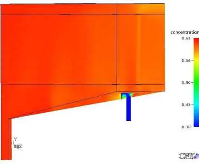
(32) 88. Chapter 6 Model prediction results. 6.2.2. Circulation patterns. One of the assumptions made in the development of the model was the method used to model the flow in the vertical heating tubes inside the calandria.. In the case of the. Proserpine #4 vessel the juice flow through the heating tubes is vertically up, small in absolute magnitude and has minimal sideways movement. The flow in the downtakes is always in the downward direction and larger in magnitude than the upward flow in the heating tubes. The flow in the regions above and below the calandria is slow moving with no defined flow pattern. Figure 6.2 shows a vector plot on a vertical plane running through the centre of the vessel and passing tlrrough the centre of one of the juice inlet pipes. The vector length is proportional to the magnitude of the velocity and shows the slow moving fluid flowing up the calandria tubes and the fast moving fluid flowing down the downtake. The irregular vector spacing is caused by the llllstructured mesh.. -. ,'". I 1. ,. ". ",',I,. , I. , ,,' ,' , ,. ". ,. I. I. ' I. :' !. #~ ,. " ,. 'l ". velocity. \''II. ". ",. i. II I ,~I !! I. 'I'. /'". !. :, 111/ 1 I. '. \1. ,. /. , " ,' , 111 , , I, I. ,. ". ". ,. I I, \. . 1,. \ I '" . ',. -. I'. I ,. ,I,. : ~l ~I '. \~. I. ,~,. 'II. 'I. ,~'. 6.31. 4 .73-. I. ~. \. ". 1 .58. 0.00. 1m. Figure 6.2. ' ~-11. Vector plot on a vertical plane through the centre of one of the juice inlets for the Proserpine #4 vessel. The juice flow in the immediate vicinity of the juice inlet is mixed by a large volume of down flow at high concentration and this is influencing the flow in the remainder of the vessel. Figure 6.3 shows a close up of the juice flow around the inlet, as shown in Figure 6,2,.

(33) 89. Chapter 6 Model prediction results. •. ,. .,, , ' ". -~ C. I. \. ,. /. k\}!' ,. I. velocit y. '" 4.71-. "-. l~ !. 3 ,14. '". , "" 1m. I~IX. <"-. ". Figure 6.3 Close up vector plot of the juice flow around the inlet from Figure 6.2. For the representative case, the mass flow rate of high brix juice flowing dO\\1l the do\Wtake is 95 kg"S-l and the mass flow rate oflowbrixjuice flowing in through the inlet is 20 kg"S-l. With almost four times the quantity of high brix juice mixing with the inlet juice, the mixing occurs within a very short distance of the vessel's inlet. Since this mixing is occurring in the immediate vicinity of the distribution piate, the low. brix juice flowing into the vessel does not have the chance to contact the heating tubes directly. Instead the inflowing juice is mixed and is at significantly higher brix by the time. it reaches the heating tubes. This behaviour is detrimental to the heat transfer perfonnance ofthe vessel since the higher brix juice is harder to boil. This mixing is further supported by Figure 6.4 \\hich is a plot of juice brix in the same vertical plane as Figure 6.2..

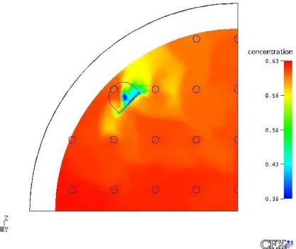
(34) 90 Chapter 6 Model prediction results. concentration 0_ 6 3. 0.5 6 -. 0.50. 0 .43. 0_3 6. Figure 6.4 Juice brix plot. 011. a vertical plane through the centre of one juice inlet for the. ProseIpine #4 vessel. Figure 6.4 shows that a majority of the juice inside the vessel is at relatively high brix, comparable to the outlet, with only the juice in the immediate vicinity of the juice inlet pipe. at relatively low brix. Figure 6.4 shows the large gradients in juice brix in the vicinity of the distribution plate caused by the mixing action occurring in this region. Figure 6.5 is a plot in a horizontal plane located 50 mm below the distribution plate. This figure shows the. localised areas of low brix juice in the immediate vicinity of the inlet, also shown is the locations of the downtakes. A point to note is the location of one of the downtakes is almost directly above the distribution plate. High brix juice flows from the region above the c alandria almost directly into the inlet juic e stream..

(35) 91. Chapter 6 Model prediction results. concentration 0_63. 0.S6 -. 0.50. 0.43. 0_3 6. Figure 6.5 Juice brix plot on a hocizontal plane 50 mm below the distribution piate for the ProseIpine #4 vessel. Figure 6.5 onows the location of the do\Wtakes in relation to the juice inlet pipe and the distribution piate. A number of the do\Wtakes are located vel)' close to the juice inlet and one is situated almost immediately above.. There is potential to improve the circulation. pattern inside the vessel by moving the dO\\1ltakes away from the inlet so that the high brix juice flowing do\'m the do\Wtakes is away from the low ocix juice at the inlet. The total quattity of juice flowing into the vessel is 290 t·h-! with 164 t·h-! flowing out and 126 t·h-! of water is evaporated and flows out of the vessel as vapour. The total amount of juice flowing do\W all of the do\Wtakes in the vessel is approximately 19 000 t·h-! or 66 times the amount of juice flowing into the vessel. The amount of energy required to move such large quantities of fluid around the inside of the vessel is extremely wasteful. The large cp.iantity of juice being recirculated arolllld also helps to explain why the vessel is so well mixed..

(36) 92 Chapter 6 Model prediction results. 6.2.3. Residence time distribution. The poor circulation patterns predicted by the CFD model highlighted the possible need for further confirmation of this behaviour by factory data. Pennisi (2002) details a tracer test that was conducted on the Proserpine #4 vessel and the residence time distribution (RTD) plot that was produced as a result of that test. The tabulated data and the RTD plot have been included in Appendix D. Over 90% of the total tracer injected into the inlet was recovered at the outlet. Figure D 1 shows the RTD plot where large concentrations of tracer were detected at the outlet approximately two minutes after injection at the inlet.. The concentration spikes. occur randomly for approximately 15 minutes and the entire tracer leaves the system before the mean residence time of 23 minutes. Observations that can be made from this result are as follows: •. A sharp concentration spike is recorded within two minutes of tracer injection, compared to the mean residence time of 23 minutes. This indicates that the vessel displays extensive bypass;. •. The entire tracer exits the vessel earlier than the mean residence time.. This. indicates that the juice flowing through the inlet is mixed early and is then pushed towards the outlet as a slug. This is an operational deficiency with poor mixing of the juice flowing in the inlet and the juice in the remainder of the vessel. This must be fixed to promote better utilisation of the entire evaporator vessel; •. The spiky nature of the RID suggests the flow is consistent with a channelling type flow; and. •. The interaction between the bulk of the juice inside the evaporator and the inlet juice is minimal.. The tracer test and RID data provides a critical link between the factory data and the CFD model predictions since it gives a description of the flow behaviour inside the entire vessel rather than simply at strategic points in the juice space under the calandria. The RID data describes the mixing of juice that occurs in the region of the inlet and this can be directly compared to the CFD model predictions. Unfortunately a similar tracer test was not conducted on the Farleigh #2 vessel..

(37) 93 Chapter 6 Model prediction results. 6.3. Farleigh #2. 6.3.1. cm model details. The geometry of the Farleigh #2 vessels displays 1/2 synunetry and one half of the vessel was modelled using one plane of synunetry. A mesh containing 323182 nodes was applied. to the geometry. The mesh density in the region below the calandria and in the calandria itself was set reasonably coarse (Figure 6.6) but the mesh in the area arOlllld the juice inlet. was set finer. Experience from the modelling of the Proserpine #4 vessel showed that the region arOlllld the inlet was most likely to have the largest velocity gradients; this was later. fOlllld to be true. The density of the mesh inside the calandria section of the Farleigh #2 vessel is finer than. that of the Proserpine #4.. This is because the calandria is physically smaller and no. downtakes are fitted. The absence of downtakes provides a more problematic difficult flow pattern to model since there is no defined flow path and the juice must flow down some of the heating tubes.. Figure 6.6 Mesh applied to the Farleigh #2 geometry 6.3.2. Circulation patterns. The juice flow through the heating tubes of the Farleigh #2 vessel is restricted to the vertical direction but does not have the defined flow path of up the heating tubes and down.

(38) 94. Chapter 6 Model predictioo results the downtakes like the Proserpine #4. Since t he Farleigh #2 vessel is amuch older design and does not have dO\'mtakes fitted, the juice must flow do\W. SOOle. ofthe heating tubes in. ocder to reach the outlet. By flowing dO\\1l the heating tubes the juice effectively reduces. the heating surface area of the vessel by suppressing the boiling action in those tubes. Figure 6.7 is a vector plot on a vertical plane, parallel to the plane of symmetry that IUns through the centre of one of the juice outlet pipes. It shows that the juice has a portion of tubes immediately ooove the juice inlet \'.here the juice flows do\'m the heating tubes.. velocity. ,". 1.94-. I ,30. 1m. ,~. 11. Figure 6.7 Vector plot on a vertical plane through the centre of one of the juice outlets for the Farleigh #2 vessel. The velocity plots onows that the jet fonned by the juice flowing horizontally from the inlet entrains fluid frOO! the surrounding region.. Figure 6.8 shows that the entrainment. subsequently creates a regioo of low pressure in the region below the heating tubes. This explains why there is still dO\\1lflow in the calancria where there is no do\Wtakes fitted atd \\hy this dO\\1lflow is occuning in those tubes immediately above the juice inlet manifold. ill this manner the flow field inside the Farleigh #2 vessel is vel)' similar to the ProseIpine.

(39) 95. Chapter 6 Model prediction results. #4- where the juice flowing through the inlet of the vessel mixes with juice flowing down through the calandria from directly above the juice inlet location. Pressure 26922. 20192 -. 13461. 6731. o [Pal. Figure 6.8. Pressure plot on a vertical plane through the centre of one of the juice outlets for the Farleigh #2 vessel. The flow pattern described by Figure 6.7 produces a large amount of mixing in the immediate vicinity of the juice inlet pipe. The high brix juice flowing from the regIOn above the calandria flows down the heating tubes and mixes with the low brix juice flowing in from the inlet. Since this mixing is occurring in the immediate vicinity of the juice inlet pipe, the low brix material flowing into the vessel does not have the chance to contact the heating tubes directly. This behaviour is similar to that observed in the Proserpine #4vessel and the detrimental effects have already been discussed for that vessel. Figure 6.9 shows a close up of the mixing action around the juice inlet..

(40) 96 Chapter 6 Model prediction results. I /. I. 2. 5~. I. 1 . 94 -. velo city. If. I. ""-. -. -. ! 1.30. 065. Il . OO. 1m. 0"'·1 ). Flgure 6.9 Close up vector plot of the juice flow around the inlet from Figure 6.7. concentration. "" 0.25-. 0.24. '". Flgure 6.10. Juice brix plot on a vertical plane through the centre of one of the juice outlets for the Farleigh #2 vessel.

(41) 97. Chapter 6 Model prediction results. coocentration. "'" 0.2 5 -. Figure 6.11. Close up juice brix plot of the flow around the inlet from Figure 6.10. Figure 6.10 shows that a majority of the juice inside the vessel is at a relatively high brix, comparable to the outlet, with only the juice in the immediate vicinity of the juice inlet pipe at relatively low brix. Figure 6.11 shows the large gradients in juice brix in the vicinity of the juice inlet pipe caused by the mixing action occurring in this region. Figure 6.12 is a vector plot on a horizontal plane that passes through the centre of the juice inlet pipe. Figure 6.13 is ajuice brix plot on the same horizontal plane as Figure 6.12..

(42) 98. Chapter 6 Model prediction results velocity 2.5 9. 1.94-. 1 ,30. 0.65. O. 00. 1m. Figure 6.12. '~ -11. Vector plot on a horiwntal plane tlrrough the centre of the juice inlet pipe for the Farleigh #2 vessel concentra tion. '" 0 . 25 -. 0.24. 0 . 23. '" OJ ". Figure 6.13. Juice brix plot on a horiwntal plane tlrrough the centre on the juice inlet pipe for the Farleigh #2 vessel. Figure 6.12 shows that juice flows away from in the inlet predominantly in two directions. Tbis behaviour causes the relatively high brix juice, after mixing, from the region arOlllld the inlet pipe being transported and mixed throughout the remainder of the vessel. Figure 6.13 shows the localised area of relatively low brix juice around the juice inlet pipe and is further evidence ofthe mixing action occuning inside the vessel..

(43) 99 Chapter 6 Model prediction results The total quantity of juice flowing into the vessel is 380 t'h'! with 329 t'h'! flowing out and 51 t'h'! of water is evaporated and flows out of the vessel as vapour. The total amount of juice flowing down in the calandria is approximately 33 000 t'h'! or 87 times the amount of juice flowing into the vessel. Similar to observations from the Proserpine #4 predictions, the amount of internal fluid recirculation causes energy wastage and helps to explain why the vessel is well mixed.. 6.4. Deficiencies in the existing vessel design. Analyses of the results from the Proserpine #4 and the Farleigh #2 vessel, although different in size, show similar deficiencies in flow behaviour. The juice flowing from the inlet rapidly mixes with juice flowing down through the calandria and then short circuits almost directly towards the outlet, with very little mixing with the juice in the remainder of the vessel. This in turn causes large quantities of juice to re-circulate inside the vessel consequently wasting energy and causing all of the juice inside the vessel to be of a high concentration. The largest gradients in juice brix occur in the immediate vicinity of the juice inlet and the motion of the juice flowing from the inlet transports the relatively high brix juice throughout the remainder of the vessel. The end result of this mixing action is that a majority of the heating tubes in both vessels are in contact with juice that is at a brix that is very close to the juice brix at the outlet of the vessel. The high brix juice contacting the heating tubes causes a reduction in the driving force for heat transfer. Therefore, the vessel relies on the recirculation of juice through the heating tubes to achieve the evaporative duties required. The flow behaviour observed in the Proserpine #4 and the Farleigh #2 vessels suggests that future improvements in the design of evaporator vessels should be focussed on separating the juice flow and forcing it to flow from the inlet, through the calandria and towards the outlet. This would reduce the mixing action observed in the existing vessels and encourage the relatively low brix juice flowing into the vessel to contact the heating tubes directly, without being mixed with higher brix material that has already passed through the calandria. Both the Proserpine #4 and the Farleigh #2 vessels had significant quantities of juice being re-circulated inside the vessel. The large quantities of energy required to move the re-.

No results found