Rochester Institute of Technology
RIT Scholar Works
Theses Thesis/Dissertation Collections
8-9-2017
Predicting underperformance from students in
upper level engineering courses
William J. Darlington
Follow this and additional works at:http://scholarworks.rit.edu/theses
This Thesis is brought to you for free and open access by the Thesis/Dissertation Collections at RIT Scholar Works. It has been accepted for inclusion in Theses by an authorized administrator of RIT Scholar Works. For more information, please [email protected].
Recommended Citation
Predicting underperformance from students
in upper level engineering courses
William J. Darlington
A Thesis Submitted in Partial Fulfillment of the Requirements for the Degree of
Master of Science in Industrial Engineering
Department of Industrial and Systems Engineering
Kate Gleason College of Engineering
Rochester Institute of Technology
Rochester, New York
Committee Approval:
Rachel T. Silvestrini, Ph.D.
Kate Gleason Chair Associate Professor Thesis Advisor
Scott E. Grasman, Ph.D.
Department Head of Industrial and Systems Engineering Professor
0 Abstract
Recent research in academic analytics has focused on predicting student performance within, and sometimes across courses for the purpose of informing early interventions. While such an endeavor has obvious merit, modern contructivist learning theory expresses an
importance on more individualized support for students. In keeping with this theory, this
research describes the development of a model that predicts student performance within a course, relative to their past academic performance. This study is done using the minimum sources of data possible while still developing an accurate model. Useful logistic models using data from the institution’s student information system, learning management system, and grade books some useful findings are developed. While each source of data was able to predict student success independently, the most accurate model contained data from both the grade book and student information system. These models were able to accurately identify students on track to
1 Introduction
This thesis presents research regarding the use of current technologies used in academia for the development of a model that will identify students that are at risk of underperforming. The goal is to work towards a predictive model that can be used to identify students who might benefit from an intervention in regards to their overall performance in a course. In the future, such a model could be built into a system that automatically generates results and sends students automated messages, warning them of their risk of underperformance. Such a system is desirable for two reasons: it could both increase instructor participation in existing student feedback systems and it would present students with information to better make decisions regarding their academic careers.
Technology and academia have a long history of interdependence. This relationship has never been more obvious than with the widespread adoption of Learning Management Systems (LMSs), the increasing commonality of online courses, and the incorporation of eLearning in curriculum [1]. A LMS is a software suite that automates the administration and tracking of educational content, such as lectures, trainings, and assessments [2]. This new landscape for learning has generated a previously unfathomable amount of data regarding the ways in which students learn and the methods professors use to teach. The relatively new field of academic analytics is now more feasible than ever and gaining considerable interest, which is largely due to the availability of data.
Academic analytics can be defined as: using data about students, teachers, and learning environments to help compare courses and institutions, allowing for better decisions regarding policies ranging from acceptance criteria to course structures [3]. Within academic analytics, there exists a focus area known as learning analytics. According to the first International Conference for Learning Analytics and Knowledge, learning analytics is “the measurement, collection, analysis, and reporting of data about learners and their contexts, for the purpose of understanding and optimizing learning and the environments in which it occurs” [4].
referenced authors, Vincent Tinto, modeled voluntary attrition rates among college students at Syracuse University. His main sources of data were from a Student Information System (SIS) (a database populated with students' personal and scholastic information), and surveys mailed to students to be completed on a voluntary basis [5]. Today, the bulk of data is collected by non-invasive sensors, meaning it is done in ways that do not interfere with, or require the
participation of students. These sources, including records stored in LMS logs, have been accepted as less biased, as well as more thorough, and thus are currently preferred over direct observation and self-reporting by students as a method of data collection [6].
With these new sources of data, some universities have set out to develop models for student performance in specific programs. Current research in learning analytics is partially driven by the potential to improve student performance within classrooms. At Purdue University, an early alert system known as Course Signals has been developed and is being introduced in select pilot classes. This system uses proprietary algorithms to predict course outcomes for individual students in real time. Within those courses' LMSs, there is an indicator that reassures successful students of their progress and warns students that are at risk of failing, allowing for corrective action to be made [7]. Within the pilot classes, Purdue has seen a decrease in dropout rates; first year retention among the 2007 test group was 96.71% in the subset that utilized Course Signals, as opposed to 83.44% in the subset that did not. This is an undeniably desirable result that may not be easily replicated due to the lack of disclosure regarding the methodology [8]. This leaves a need for research regarding the development of a transparent predictive model of student performance, which may to encourage widespread adaptation and adoption of these types of models.
This need is highlighted by the existence of alternative programs that allow professors to manually mark students as being at risk of failure and notify the student, the student's advisors, and other professors. It is well documented that providing feedback of this nature helps student's feel empowered, which is a key attribute for an effective learning environment [9]. The
institution being examined in this study currently utilizes such a system (Starfish EARLY
low exam scores, or attendance issues. When flagged the student is notified, along with instructors for their other courses and faculty in their department.
The institution examined in this study requires for faculty participation, it is unenforced so its use varies by department, professor, and even course. Additionally, this is a
time-consuming process for professors, and the accuracy of the predictions of failure is dependent on their experience teaching and the extent of their interactions with each individual student. An automated alert system would serve to both increase the quality of the service and decrease the number of man-hours it requires.
While it is important to identify a student who is possibly at risk of failing a course, there are other students not at risk of failing who might also benefit from feedback. According to Hattie and Timperley, feedback is needed to explain the discrepancy between desired
performance and actual performance [9]. Consider the “straight A” student that receives a C in a course. While the student did not fail, they will likely be unsatisfied with their grade relative to their past performance. This example illustrates the need to broaden the qualifications for students in need of feedback. Keeping with the understanding of feedback’s purpose from Hattie and Timperley, this study will define a student’s need for feedback based on the discrepancy between a student’s past performance and their performance in the course being modeled. This method still requires that the students’ course performance be modeled which has its own set of challenges.
One of the challenges in developing a predictive model for course performance is selecting the correct features, or variables, to be included in the model. Past studies provide some insight into what variables may be statistically significant factors for predicting student grades. In many models, a student's cumulative grade point average (CGPA) is used as a factor, as it is an accessible measure of a student's typical performance in the classroom [10–13]. In addition to a measure of average academic performance, some researchers have attempted to include estimates of subject matter knowledge.
method of capturing subject matter knowledge is to examine the student's performance in
prerequisite courses. This can simply include the grade earned in a prerequisite class or it may go further to include the time elapsed between the prerequisite and current course [14].
Additional variables that have proven useful for predicting course performance are gender, age, and seating location. Unfortunately, there remains other information that is potentially relevant to student performance that cannot be directly measured, such as student interest and learning style. For these intrinsic factors, surveys remain a primary means of data collection due to the inability to effectively capture the information otherwise, but great care must be put into their design and administration [15]. Despite abiding by the rigorous
requirements of administering one of these surveys, they remain subject to the biases inherent to self-reporting. For this reason, data available in LMSs has been used to supplement survey data, and sometimes replace it all together [6].
Using data typically captured by an LMS, researchers have quantified two student
behaviors that play a role in success in classes: procrastination and engagement. In a 2015 paper, You [16] utilizes absences from class and late submissions of assignments as behavioral indicators of procrastination, and shows a correlation with their occurrence and lower course grades [16]. Junco and Clem use frequency of highlighting in conjunction with average duration of access and regularity of access of digital textbooks to quantify engagement, which shows a positive correlation with course outcomes [6]. Additionally, there has been significant research into methods of evaluating the various learning management systems that are available to colleges and universities. Consideration has been given to administrative ease, cost, user interface, and even the individual tools available within each system [17]. At an individual course level, Wilson and Fowler found that organizing classes to match an active-learning pedagogy resulted in students practicing more “deep learning” techniques [18]. This is an important finding because it shows that the way a professor organizes a class can impact a student's depth of understanding of a topic, and by extension their performance in that course, and thus, may be a possible predictor of performance.
impact on their CGPA. This framework involves the development of predictive models
constructed utilizing survey data, historical data on academic performance, in-course assessment results, and LMS usage statistics. Models were generated using data restricted by the date it became available to investigate how the models, and predictions, change as a course progresses. It is expected that the accuracy of these predictions will improve as the course progresses, as demonstrated by Olama in a 2014 study of massive open online courses (MOOCs)[19]. While accuracy is important, the benefits of predicting course outcome lessen cover the timeframe of the course as there is both less time for corrective action to be taken and typically fewer degrees of freedom in the course grade. For this study, focus will be given to the weeks in which the institution being studied currently encourages instructors to identify at risk students.
This paper is divided into six sections: an introduction, literature review, data and
limitations, methodology, results, and discussion. The literature review presents past research in the field of learning analytics, highlighting the gaps between and shortcomings of the studies. The Data and Limitations section explains how the data was collected for the study as well as the difficulties and limitations associated with them. The methodology is broken into two
subsections, the first explaining how variables were transformed and used to generate new variables, and the second to explain how models were generated. The results section presents and explains the models created by following the methodology, and the discussion section interprets those results, drawing conclusions about students and suggesting next steps to take this research further.
2 Literature Review
This section summarizes selected past research in learning and academic analytics. The literature covered has provided guidance for this study in terms of what strategies have shown promise when predicting course outcomes, as well as showing challenges and shortcomings of past student performance research.
duration, frequency, time of access, and a proprietary metric called Engagement Index. Using these factors along with simple student demographic information and GPAs, the researchers performed blocked hierarchical linear regression to predict course grades, the subsequent model had an R2 value of 0.254 [6]. These findings are significant in that they suggest both that LMS usage statistics have the potential to develop proxy measurements of student behaviors, and that student behaviors can be used as predictors of student performance.
These findings are further supported by research on predicting outcomes of online courses. Zacharis found that of the 29 different usage statistics recorded by the LMS he was examining, just 4 were needed to predict 52% of the variance in student grades [20]. However, the variables used were only summaries of each student’s usage statistics throughout the course, thus they were not an accurate representation of the students’ week-to-week behaviors.
Furthermore, it is important to acknowledge that the courses in that study were entirely online, not blended courses like those being examined in this study.
for regimented classes with frequent and consistent graded assignments.
Other research has ventured to predict students final course grade even before they set foot in the classroom by using previous scholastic achievement. In a 1992 study,
Danko-McGhee and Duke modeled student success in an intermediate accounting class using their grade in an introductory accounting course and the number of semesters that had passed between being enrolled in the two classes as input variables. These two features were determined to be more statistically significant than the other variables included in the model: cumulative GPA and score on a diagnostic exam. Overall, the study’s linear model explained 41.6% of the variance in students’ grades for the intermediate accounting class [21]. While the study did not result in an exceptionally accurate model, it successfully shows the predictive power of student's past performance for their future performance indicating it as a potentially valuable factor in a more comprehensive model.
While variable selection is critical to predictive modeling, there are many different statistical techniques that can be employed to generate the actual model. Past research in predicting student performance has shown the usefulness of various methods, depending on the response variable being modeled and the intended use of the models. Fang & Lu showed the merit of a structured decision tree in predicting the letter grade of a course in a 2010 study [22]. Multiple linear regression is an often used method when predicting student grades on continuous scales, for it’s simplicity and interpretability [11, 13, 20]. However, most aligned with the goal of this research is logistic regression, with Macfayden and Dawson demonstrated as an effective means to model “risk of failure”, in a proof of concept for an “early warning system” [23].
This study will use the findings of past works and a basic understanding of modern learning theory to select variables to be collected and later used in modeling. Based on
that attempt to do so across multiple classes and even subject matters. Recently, Gasevic et al. Showed that predictors of success not only vary by course, but when universal models are made for multiple courses new predictors show significance [24]. These findings highlight the ease of over fitting models to the learning process. To help mitigate over fitting, and forced significance of variables, the number of variables included in the model was extremely limited and many that were included were known to have correlation with the final course grade.
3 Data and Limitations
This section will outline precisely how data was collected for this study, how that data was cleaned, and a brief discussion of the challenges associated with some of the data.
Limitations of the metrics collected from each source are discussed in the subsections when relevant. Visualization of the various data sets is presented, along with interpretations of those visualizations. The data analyzed in this research came from two sections of a cross-listed engineering course at a large private institution in the North Eastern United States. The sections were taught by the same instructor however the syllabus and course structure did change between sections. The sections were taught in the Fall semesters of 2014 and 2015.
3.1 Learning Management System Data
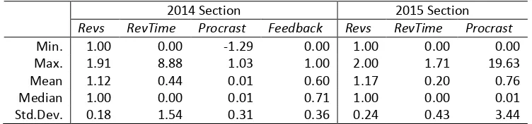
The first data source examined in this study was the learning management system (LMS). Within this research, the LMS data collected primarily pertains to assignments within the class being analyzed. For each assignment, the number of submissions a student made (Revs) and the time elapsed between the first and subsequent submissions (RevTime) were interpreted as theoretical measures of how much a student revised their own work. In a similar method, the number of hours before a deadline that a student made their first submission for an assignment was treated as a measure of procrastination (Procrast). Also recorded was whether or not a student read any feedback posted on their assignments. This variable was measured as a percentage of the available feedback viewed at any given day (Feedback). Unfortunately, the 2014 section of the course did not distribute feedback digitally, and thus the measure was unavailable for that section.
students view course material. The metrics included the first date of access, the number of accesses, the last access, and the total duration of access for any given set of course notes, handouts, or other electronically distributed information. While potentially valuable, this information was stored cumulatively rather than periodically with time stamps. Consequently, there were no accessible measures of access patterns for, or up to, a specific week. Instead, only the summaries of the access patterns for the entire semester were available. For this reason, it was impossible to accurately derive the patterns of course access after the course was completed. Since this research aims to provide a method to identify students in need of feedback during a course, reflexive summary statistics of access patterns could not be used.
Table 1 shows the minimum, maximum, and median values for each of the LMS variables divided by course section. These summary statistics show the similarities and differences in these variables between sections. Note that the median and minimum values remain consistent across the sections while the other values change. This suggests that the typical student in each section is similar, but the outliers of each section are not consistent.
Table 1: Contained in this table is the summary statistics of data collected from the LMS for both the 2014 and 2015 sections of the course being studied.
2014 Section 2015 Section
Revs RevTime Procrast Feedback Revs RevTime Procrast
Min. 1.00 0.00 -1.29 0.00 1.00 0.00 0.00
Max. 1.91 8.88 1.03 1.00 2.00 1.71 19.63
Mean 1.12 0.44 0.01 0.60 1.17 0.20 0.76
Median 1.00 0.00 0.01 0.71 1.00 0.00 0.01
Std.Dev. 0.18 1.54 0.31 0.36 0.24 0.43 3.44
3.2 Student Information System Data
In addition to the LMS data, data regarding the academic record of each student was collected from the university’s student information system (SIS). The course being analyzed for performance prediction required completion of two prerequisite classes for enrollment,
“Introduction to Probability” and “Introduction to Statistics”. The final letter grade (A, B, C, D, or F) was collected, along with the academic term in which it was completed. Students that completed the prerequisite courses at another institution, before matriculation or otherwise, were marked with a grade of T. In conjunction with the grade each student earned in these
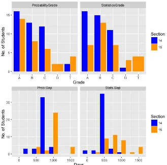
[image:14.612.138.467.370.694.2]prerequisite courses, the number of days from the completion of the prerequisite courses to the start of the course under study was measured. These variables (Prob.Gap and Stats.Gap) served as a measure of how “fresh" these fundamental topics were in the students’ minds. The student at status gap 0 was enrolled in the mandated prerequisite while taking the course under study. These variables are summarized in Figure 1.
As Figure 1 indicates, the 2014 section of the course had more uniform and consistent grades across the two prerequisite courses than students in the 2015 section. Figure 1 also indicates that most of the students in the 2014 section enrolled in the prerequisites at the same time, suggesting that they may have been enrolled in the courses with each one another. The histograms also show that the 2015 section earned lower letter grades in “Introduction to
Statistics” than they did in “Introduction to Probability”. Most students in the 2015 section took “Introduction to Probability” at the same time, whereas their enrollment in “Introduction to Statistics” was much less consistent.
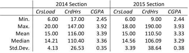
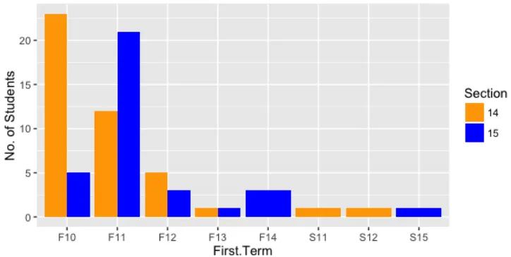
[image:15.612.148.466.518.608.2]In addition to information regarding prerequisite courses, general academic statistics were collected. The variables recorded were: cumulative grade point average (CGPA), to represent general academic aptitude; enrolled credit hours during the term of the course being studied (CrsLoad), to capture the rigor of their other academic commitments; total completed credit hours up to the term of the studied course (CrdHrs), and the term when each student first matriculated into the university (FirstTerm), to quantify academic experience.
Table 2 shows the minimum, maximum, and median values for each of the variables from the SIS pertaining to general academic history. These summary statistics show the similarities and differences between these variables in different sections. Note that the mean and median values are similar between the sections, while the minimum, maximum, and standard deviations show greater differences. This indicates that the 2015 section had a larger variety of students, while still remaining similar to the 2014 section on average.
Table 2: Summary statistics for continuous variables collected from SIS pertaining to both the 2014 and 2015 Sections of the course being studied.
2014 Section 2015 Section
CrsLoad CrdHrs CGPA CrsLoad CrdHrs CGPA
Min. 6.00 17.00 2.45 6.00 9.00 2.44 Max. 20.00 147.00 3.92 18.00 190.00 3.93 Mean 15.00 116.00 3.39 15.00 110.50 3.33 Median 14.21 110.40 3.36 14.56 106.09 3.29 Std.Dev. 4.13 26.53 0.35 3.39 38.64 0.38
students from the 2014 section, indicating similar academic timelines between students in either section. Furthermore, the matriculation dates for students in the 2014 section
follow a more predictable pattern than those for the 2015 section. However, after examining the raw data, CrdHrs was taken as a less biased indicator of academic experience than a
chronographic measure, such as the number of months as a matriculated student, because of the irregularities in collegiate schedules, such as transfer students and graduate students.
In order to quantify the rigor of a student’s semester, the number of credit hours they were enrolled in during the course was recorded as a variable (CrsLoad). While credit hours may not fully quantify the difficulty of a course, alternative options had similar shortcomings and introduced new sources of bias. One alternative approach was to weight the credit hours of each course by the course number. This approach would consider a three credit 100-level course to be a lesser workload than a three credit 400-level course. However, to implement such a weighting system would require a (possibly arbitrary) evaluation of the relative difficulty of different course levels and implies that higher-level courses are always more demanding than lower-level courses, an assumption without empirical support.
3.3 Survey Data
[image:16.612.120.482.209.391.2]The final source of data utilized in this study was an in-person survey distributed to students. This survey included 15 questions that attempted to quantify information descriptive to each student’s situation and study habits not available by existing digital means. The survey, in
its entirety, is available in the Appendix. The survey distribution was limited to only courses that took place during 2015, when this study commenced. There is no survey data available for the first section of the course under study, thus the survey data was not used in the final predictive modeling, but it’s analysis provided some valuable insights into student behaviors.
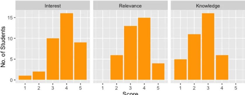
Figure 3 shows the students ranking of their interest in the course, perceived relevance of the course, and previous knowledge of the subject matter as determined by their survey
responses. These charts show that most students enrolled in the course with at least a basic understand of the material. It also shows that perceived relevance was has a fairly symmetric distribution with the mean falling between 3 and 4, suggesting that the students see some value in learning the material. Lastly, the histograms show the interest in the subject matter was centered on 4 with very few students showing little to no interest in the material. This suggests that most of the students would derive some internal motivation to learn the material.
The survey also asked students to self-report their allocation of time to both studying and extracurricular activities, including work and athletics. Figure 4 shows each students allocation of time in hours, sorted from left to right by time dedicated to extracurricular activities. This plot suggests that there is no clear correlation between the time that a student spends studying and the time that they spend dedicated to extracurricular activities. Furthermore, no students spend more than ten hours a week studying for the course, and that extracurricular commitments range from 0 hours a week to the equivalence of a full-time job at 40 hours per week.
Figure 3: Student responses to survey questions asking them to rank their interest in the course, perceived
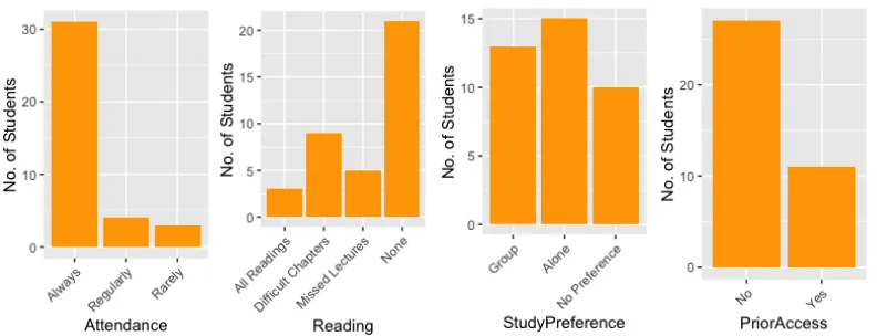
Questions about the students’ habits specific to the course under study were also asked in the survey. Students were asked to self-report their class attendance, completion of the
suggested readings, preference to study with a group or individually, and whether they had access to the course materials prior to the class’s start. The results to these questions are illustrated in Figure 5. These charts show that nearly half of the students never did any of the suggested readings for the course and very few students did every reading. Students’ preferences for studying independently were evenly split with 34% preferring groups, 39% preferring
[image:18.612.107.506.73.274.2]studying alone, and the remainder having no preference. A significant portion of the class, 29%, had access to course materials before the course began.
Figure 4: Student time allocation to studying, as compared to extracurricular activities.
Figure 5: Student habits with regard to the analyzed course. From left to right the histograms
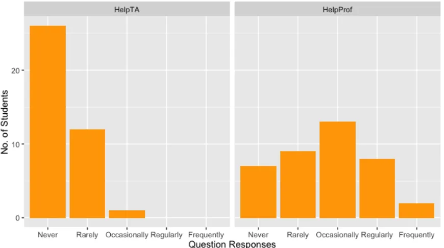
[image:18.612.100.496.508.660.2]Lastly, the survey attempted to measure self-advocacy in the course. To do this, students were asked how often they asked the teaching assistants and instructor for help. The responses are plotted in Figure 6. These plots show that most students did not go to teaching assistants for help, and those that did, did so rarely. Students were much more likely to ask for help from the instructor. The histogram shows that only seven students never got help from the professor and more than half the class went to the professor for help at least occasionally. This indicates students believe the professor was both willing and able to help them better perform in the class, giving hope for the effectiveness of an intervention.
3.4 Data Cleaning and Challenges
[image:19.612.85.520.255.498.2]Once data from all four of these sources was collected and organized into data tables, it was checked for completeness. Three students who did not have values for the majority of the variables were discarded, as they could not be modeled with the same dimensionality as the other students. Once complete cases were gathered, each of the numeric features was scaled to allow for comparison. When predefined bounds to the variables existed, such as exam grades (0-100), they were utilized. In all other cases, such as CourseLoad, the maximum and minimum observed values in the section were used as the bounds. Table 3 presents a list of all variables collected for
Figure 6: Summary of the frequency at which students request help from both the teaching assistant and
the study.
Outside of the challenges in interpreting the various metrics collected, this study was hindered by a policy change at the university that occurred within the span of the study.
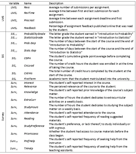
Table 3: This table contains all of the variables collected for this study, as well as their abbreviations and brief explanations.
Variable Name Description
LM
S
LMS1 Revs Average number of submissions per assignment.
LMS2 RevTime Average time between first and last submission for each assignment.
LMS3 Procrast Average time between each assignment deadline and first submission.
LMS4 Feedback Percentage of assignment feedback published online that was read by the student.
SI
S
SIS1.1 ProbabilityGrade The letter grade the student earned in "Introduction to Probability"
SIS1.2 StatisticsGrade The letter grade the student earned in "Introduction to Statistics"
SIS2.1 Prob.Gap The number of days between the start of the course and the end of "Introduction to Probability"
SIS2.2 Stats.Gap The number of days between the start of the course and the end of "Introduction to Statistics"
SIS3 CGPA The student’s cumulative grade point average before completing the course.
SIS4 CrsLoad The number of credit hours the student was enrolled in at the time of taking the course.
SIS5 CrdHrs The total number of credit hours completed by the student at the start of the course.
SIS6 FirstTerm Academic term that the student matriculated into the university.
Su
rv
ey
Surv1 Interest The student's self reported Interest in the course.
Surv2 Relevance The perceived relevance of the course to the student.
Surv3 Knowledge The student's self reported prior knowledge of the course's subject matter.
Surv4 ExtraCurr The number of hours the student dedicates to extracurricular activities on a weekly basis.
Surv5 StudyHours The number of hours the student dedicates to studying the subject matter on a weekly basis.
Surv6 Attendance The student's self reported attendance to the course.
Surv7 Reading The student's self reported frequency of reading suggested materials.
Surv8 StudyPreference The student's preference, or lack thereof, to study individually or with a group.
Surv9 PriorAccess Whether the student had access to course materials before the class began.
Surv10 ProfHelp The student's self reported frequency of seeking help from the instructor.
Surv11 TAHelp The student's self reported frequency of seeking help from the teaching assistants.
4 Methodology
techniques were employed to create predictive models discussed in the results section.
4.1 Variable Creation
In past research such as those presented in the literature review, the typical response variables for student performance modeling are numeric grade, 0-100; the categorical letter grade; A, B, C, D, or F; and the Pass/Fail binary outcome. While these responses are accurate to the empirical metrics of student success, such approaches rely on instructors determining which response values require intervention. To eliminate the need for instructors to choose
performance thresholds for each student, this research engineered a response variable based on the students past academic performance.
The response variable developed was a binary measure indicating whether or not the student’s cumulative GPA (CGPA) would be negatively affected by the grade they earned in the course being modeled. To do this, the course grade, as a percentage, had to be converted to a 4-point scale. Typically, percentages are converted first to a letter grade, then to the corresponding number on the scale from 0 to 4. However, it is not uncommon for instructors to adjust a letter grade when converting it from a percentage. In other words, an instructor might give a student that scored an overall grade of 89/100 in the course an A during one semester and a different student who scored an 89/100 a B during a separate semester. Additionally, different instructors might have different definitions failing percentage. For courses where students typically earn higher grades the failing percentage might be 75%, and in courses where students typically earn lower grades the failing percentage might be 50%.
To generalize the transformation from a percentage to a four-point scale, a linear
communicating with the instructor on a regular basis.
Equation 1 shows how the course grade is converted to a four-point scale, depending on what percentage is determined to be a failing grade.
!= 𝐶𝑜𝑢𝑟𝑠𝑒𝐺𝑟𝑎𝑑𝑒100−𝐹𝑎𝑖𝑙𝑖𝑛𝑔𝐺𝑟𝑎𝑑𝑒−𝐹𝑎𝑖𝑙𝑖𝑛𝑔𝐺𝑟𝑎𝑑𝑒
4
Equation 1
The scaled course grade,Ψ, is then weighted by the number of credit hours the course is worth and averaged with the students CGPA weighted by the total number of credits they have completed.
𝐶𝐺𝑃𝐴!"# =
𝑇𝑜𝑡𝑎𝑙𝐶𝑟𝑒𝑑𝑖𝑡𝑠 𝐶𝑃𝐺𝐴!"#$ + !𝐶𝑜𝑢𝑟𝑠𝑒𝐶𝑟𝑒𝑑𝑖𝑡
𝑇𝑜𝑡𝑎𝑙𝐶𝑟𝑒𝑑𝑖𝑡𝑠+𝐶𝑜𝑢𝑟𝑠𝑒𝐶𝑟𝑒𝑑𝑖𝑡
Equation 2
The new CGPA was then compared to the original CGPA. If there was a decrease greater than the determined tolerance, or the scaled course grade was below 1, then AffectedGPA
was 1. If the scaled course grade is greater than 3, then AffectedGPA was 0.
𝐴𝑓𝑓𝑒𝑐𝑡𝑒𝑑𝐺𝑃𝐴= Ψ<1 ∨ 𝐶𝑃𝐺𝐴!"#$−𝐶𝑃𝐺𝐴!"# > 𝑇ℎ𝑟𝑒𝑠ℎ𝑜𝑙𝑑 ⋀[Ψ< 3]
Equation 3
While this method does programmatically create a response unique to each student, it still requires a manually set tolerance for an acceptable decrease in CGPA, which presents an
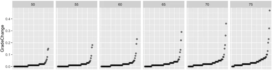
opportunity for error by the instructors. However, rather than using an entirely arbitrary range, one could potentially be selected empirically based on scores in past sections. To do this, the differences between 𝐶𝑃𝐺𝐴!"#$ and 𝐶𝑃𝐺𝐴!"# were plotted in ascending order. In Figure 7, the
A sensitivity analysis was performed to determine how changes in the conversion from grades as a percentage to a letter grade would affect the changes in students’ CGPAs. Adjusting the lower limit for a passing grade from 50% up to 75% increased both the number of students who had their CGPA decreased and the amount by which their CGPA decreased. Knowing this, the range for what decrease in CGPA is acceptable could be changed when generating predictive models. The calculated CGPA decreases are plotted in Figure 7, showing the increased effect on students CGPA as the threshold for failure is increased.
As mentioned in Section 3, individual assignment grades were not used as variables when modeling student success. Rather, assignment grades were used to generate new variables to be utilized for modeling. This was done to lower the chances over fitting a model to a specific class or section of a class. The first variable created regarding student grades is a simple running average (HWAvg). This variable is easily calculated and represents a student’s general
performance on assignments, rather than their understanding of specific material. The standard deviation of homework grades was also calculated as a potential variable for explaining student performance (HWSD). This feature would theoretically represent how consistently each student performed across different units of the course.
[image:24.612.76.537.92.211.2]Taking these engineered variables further, in an attempt to make a more accurate representation of how a student is performing on homework more advanced algorithms were applied to the grade data. The existing grades were used in a moving average model that predicted what their homework average would be after 16 weeks, the total length of the course. The resulting value for each student was used as a variable when modeling student success (ProjectedHW). However, the moving average modeling method was unstable when less than
Figure 7: The plot shows the negative changes in student's Cumulative GPAs based on their course
four homework grades were available for training the model to create the projected homework variable. This limited the variable’s existence to approximately halfway through the course. Using the same modeling technique, a second feature was extracted. This feature was developed with the aim of replacing HWSD. Its calculation is simply the margin of error for the prediction generated by the moving average model (ProjectedError). This variable was expected to be a measure of how unstable the student’s homework average was, thus indicating students that might see a sudden drop in homework average.
Another new variable was created based on the grades students earned in the prerequisite courses. With the sample size being small relative to the number of variables being considered for modeling, over fitting was a concern. To combat this, the variables ProbabilityGrade and
StatisticsGrade were changed from categorical variables with five factors to binary variables indicating whether an A was earned in the class, reducing the dimensionality of the model by eliminating six possible dummy variables. Further manipulation was done to make a variable less specific to the course being studied. To do this, the sum of the two variableswas calculated and divided by two. This new variable, AinPrereqs, is the portion of the prerequisite courses that the student earned an A in.
The last engineered variable was a basic summation of two other variables. This was done in order to lower the dimensionality of the models and prevent the use of two highly correlated variables in the model. Reducing the dimensionality also decreases the chances of over-fitting and improving predictive performance on new data. The variables combined were
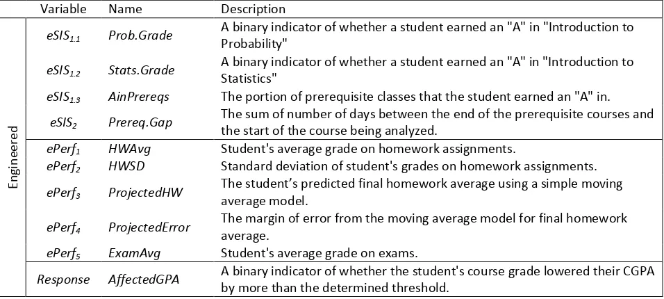
Table 4: This table contains all of the variables developed in this study, as well as their abbreviations and brief explanations.
4.2 Analytical Techniques
This section details the modeling process used in this study. The data, collected and transformed, as described in Sections 3 and 4.1 respectively, was analyzed and used to train predictive models. Logistic regression, as described by McCullagh and Nelder in Generalized Linear Models, was selected as the method of modeling the binary response variable,
AffectedGPA [25]. In order to identify which of the many variables were significant and strong predictors, stepwise logistic regression was employed, as outlined in Modern Applied Statistics with S [26]. In conjunction with the stepwise methodology further steps were taken to simplify and generalize the resulting models.
The data was broken into blocks based on the source it was collected from, the blocks were then further divided by the week in which the collected data represented. From here additional cumulative data sets were created, containing all of the individual weeks’ data. The cumulative data sets allow for a single model to be fit to the entirety of the course, rather than individual models for each week. With data from each source divided into slices of each week and a cumulative slice, it was then replicated to account for the variability of the response variable.
Variable Name Description
En
gi
ne
er
ed
eSIS1.1 Prob.Grade A binary indicator of whether a student earned an "A" in "Introduction to Probability"
eSIS1.2 Stats.Grade A binary indicator of whether a student earned an "A" in "Introduction to Statistics"
eSIS1.3 AinPrereqs The portion of prerequisite classes that the student earned an "A" in.
eSIS2 Prereq.Gap The sum of number of days between the end of the prerequisite courses and the start of the course being analyzed.
ePerf1 HWAvg Student's average grade on homework assignments.
ePerf2 HWSD Standard deviation of student's grades on homework assignments.
ePerf3 ProjectedHW The student’s predicted final homework average using a simple moving average model.
ePerf4 ProjectedError The margin of error from the moving average model for final homework average.
ePerf5 ExamAvg Student's average grade on exams.
The response variable, AffectedGPA, is dependent on both the instructor’s standard for passing the course and the chosen tolerance for CGPA decrease. To understand how those changes affect the response variable, a sensitivity analysis was performed on AffectedGPA. From the sensitivity analysis, five possible combinations of grading conditions were selected and applied to the replicated data slices. From here stepwise logistic regression was performed on each data slice independently.
With five models fit to each slice of data, there was notable variation between models suggesting that the models were not well generalized. To further generalize the models, the statistical significance of each variable in all of the models across each data source was
examined. This resulted in eighty different models for each source of data, each with different coefficients and significant variables. From this list of eighty models, only the variables that appeared most frequently and consistently were kept, helping to ensure more generalized models.
The resulting fitted values from the logistic models, are the probabilities that the student will have a significant decrease in CGPA, indicated by a positive value of Affected GPA. In order for that continuous response to be used to students as needing an “early alert” or not, thresholds for each model was set. For example, if the threshold is set at 0.5, then any predicted probability above 0.5 would receive a 1, and those at or below 0.5 would receive a 1. If these models were put into practice than the students who received a predicted change of 1 would be flagged for risk of under performance.
Using the Error Score the classification threshold was calculated using three fold cross-validation. The data slices were randomly split into thirds, with two parts being used to train the model, and the remaining third being used to test the result. The fitted values for the test sets were then classified based on an arbitrary threshold, and the error score was calculated as described above. The threshold was incremented from zero to one, with the error score for each threshold being stored. This was then repeated 100 times, with different random samples being used for training and testing of the models. The threshold that resulted in the lowest average error score was selected as the optimal threshold for that given model.
5 Results
This section presents the results of the sensitivity analysis performed on the response variable (AffectedGPA), discusses the models that were trained for each source of data, and contains the results of the threshold optimization. Rather than presenting the models for every week, only the models generated for the weeks in which the institution requires “EarlyAlerts” are shown. The resulting models and thresholds are validated as to ensure logical and sensible results.
To ensure that the response variable is appropriate and rational, a sensitivity analysis was performed using the actual data. Taking the percentage grades earned by each student across all section of the course, the minimum passing grade, and tolerance for CGPA decrease were adjusted. For each combination of minimum passing grade and CGPA decrease, the number of students classified as having a positive value for AffectedGPA was recorded, Table 5 shows the results. There is a trend showing that when an instructor sets a higher standard for passing in a course, more students will experience decreases in CGPA and those decreases will be larger. As the tolerance for CGPA change was increased, the number of flagged students decreased
Table 5: Number of students classified as having a significant decrease in CGPA based on the course’s minimum passing grade and the tolerance for CGPA decrease. Conditions that have been modeled in the remainder of this study are marked with an asterisk.
Min. Passing
Grade
Acceptable Decrease in CGPA
0.00 0.01 0.02 0.03 0.04 0.05 0.06 0.07 0.08 0.09 0.10 0.20 50% 41 41 19 8* 6 5 5 4 4 3* 3 1 55% 48 48 23 12 7 5 5 5 4 4 3 1 60% 53 53 29 16 9 8 7* 7 7 7 6 4 65% 60 60 36 24 16 8 8 8 8 8 8 6 70% 66 66 47 28* 22 16 10 8 8 8* 8 6 75% 71 71 55 39 27 23 20 18 17 16 16 16
These groupings show that students in classes with higher standards for success should expect the potential for a larger negative impact on their CGPA. In the scope of this research, this table allows instructors to appropriately calibrate the range of an acceptable decrease in CGPA, based on what their standards of success are, and approximately how many students they feel capable of providing effective follow-up and feedback to. For example, if an instructor does not have the resources to provide meaningful additional support to 20 students, they may
consider lowering the minimum passing grade, or anticipating the possibility of students seeing larger decreases in their CGPA.
5.1 Modeling Student Information System Data
Using data collected from the SIS, only the cumulative data was examined because the SIS data used in this study remained constant throughout the course. Initially using all the SIS
and eSIS variables, the modeling process as described in Section 4.2 was followed. Including all of the SIS variables in stepwise regressions for each week of data, only the variables that most consistently showed statistical significance were kept for the models discussed in this section. This process of variable selection resulted in only two variables remaining, SIS3and SIS5. The formulation of the model with the response variable based on the most lenient grading conditions is shown in Equation 4. This equation directly calculates the probability of a positive response variable.
𝑃 𝐴𝑓𝑓𝑒𝑐𝑡𝑒𝑑𝐺𝑃𝐴 = 100%
1+𝑒!(!".!"!!.!" !"!!!!".!!"!!)
Equation 4
An alternative formulation of the same model is shown in Equation 5. This alternative form calculates a logistic odds ratio, or logit, rather than a probability. In doing so it makes for an easier interpretation of the variables and their coefficients. A lower logit indicates a smaller probability of a positive response for AffectedGPA and a larger logit indicates a larger
probability. When the logit is equal to zero there is 50% chance of a positive response for
AffectedGPA.
log 𝑃 𝐴𝑓𝑓𝑒𝑐𝑡𝑒𝑑𝐺𝑃𝐴
1− 𝑃 𝐴𝑓𝑓𝑒𝑐𝑡𝑒𝑑𝐺𝑃𝐴 = 16.82−4.64𝑆𝐼𝑆!−13.2𝑆𝐼𝑆!
Equation 5
To interpret the model, consider Equation 5. The variables and their coefficients have a linear relationship with the logit. When SIS3 or SIS5 increases, the logit decreases, when SIS3 or
SIS5 decreases, the logit value increases. Furthermore, it can be seen that a one unit change in
SIS3 has a smaller affect on the logit than an equivalent one unit change in SIS5 based on the magnitude of their respective coefficients. This method of interpretation and the relationships between magnitude and direction of coefficients can be applied to all of the logistic models in this and the following sections.
shown in a tabular form in Table 6. Every iteration of the models have negative coefficients associated with both SIS3 and SIS5. This indicates that students with lower CGPAs and less completed credit hours are more likely to have a positive value for the response, AffectedGPA. This is inline with what was hypothesized, that student’s with lower CGPAs are more likely to earn a D, or a failing grade in the course. Likewise, students with fewer completed credit hours both have more easily decreased CGPAs based on the method by which it is calculated, and they have a less established academic performance, so even those with higher CGPAs may still be susceptible to an unexpectedly low grade.
Examining the AIC of the models for each set of grading conditions, it is clear that the instance in which the minimum passing grade was the highest and the tolerance for CGPA decrease was the lowest was the worst fit. This can be attributed to the large number of students being labeled with a true positive response variable. In the remaining instances the AICs are significantly lower, reaching its lowest value under the conditions in which the fewest students were labeled with a true positive response variable. Interestingly, the second model has a higher AIC than the fourth model despite having the same number of students labeled with true
[image:31.612.104.476.500.617.2]positives. This is likely attributable to more students receiving a D or F in the fourth model, where as the second model relied more on actual decrease in CGPA to flag students with a positive response variable.
Table 6: Logistic regression model using variables collected from the institution's student
information system. Min. Passing Grade CGPA Change Tolerance
Week Coefficients AIC
Intercept SIS3 SIS5
50% -0.09 All 16.82*** -4.64*** -13.20*** 196.07 50% -0.03 All 11.38*** -2.85*** -9.05*** 508.37 60% -0.06 All 28.01*** -7.26*** -17.21*** 284.50 70% -0.09 All 21.31*** -5.55*** -12.83*** 392.63 70% -0.03 All 9.80*** -2.49*** -4.16*** 1233.50 Statistical Significance codes: ‘***’ 0.001 ‘**’ 0.01 ‘*’ 0.1 ‘^’ 0.3
because they have the tightest groupings of true positive points. The marginal difference between the second and fourth models becomes more clear with the fourth model having fewer true positive observations with low fitted values. The first model, with the most lenient grading conditions, shows that none of the students with a fit probability of zero had a significant decrease in CGPA. However the nearly constant response variable suggests over fitting. The third model, with the median grading conditions, is similar although there is more variation in the response variables, suggesting that the over fitting is less dramatic. In the case of the second, a fourth, and fifth model there does not appear to be over fitting. The second model has a few true positive responses with low fitted probabilities, showing its inaccuracy. The fourth model successfully separates most of the true positive observations from the true negatives, with the exception of two observations that had relatively low fitted values. The fifth model has an indiscernible range of probabilities fit to true positive observations, indicating that it has little value for classification.
5.2 Modeling Learning Management System Data
The university’s learning management system data was used to create models. After performing stepwise regression across all of the slices of LMS data and comparing the results, only Procrastination was kept in the model because it consistently showed statistical
significance. As seen shown in Table 7, all of the models resulted in negative coefficients for the
[image:32.612.77.529.342.456.2]Procrastination, which implies that students who submitted their assignments earlier, had a lower chance of having a negatively affected GPA. This is aligned with what was hypothesized, that students who do work early perform better than those who are rushed when completing their assignments. However, as indicated by the asterisks, or lack there of, Procrastination had fairly
Figure 7: This figure shows the fitted values for models generated using only data from the student information
high p-values in most models, with the exception of the cumulative models.
Table 7: The table below shows the models fit to week 7, week 12, and all the weeks of data collected from the
learning management system. Asterisks indicate statistical significance of the terms, and the Akaike information criterion is included for each model.
Min. Passing
Grade
CGPA Change
Tolerance Week
Coefficients
AIC
Intercept LMS3
50% -0.09 All -1.64*** -5.75*** 331.17
50% -0.09 7 0.74 -13.93* 23.30
50% -0.09 12 1.52 -12.86* 22.15
50% -0.03 All -1.59*** -1.68*** 753.34
50% -0.03 7 -0.84 -3.79^ 53.41
50% -0.03 12 -0.70 -3.33^ 53.74
60% -0.06 All -1.75*** -1.66** 687.66
60% -0.06 7 -1.46^ -2.34 50.15
60% -0.06 12 -0.91 -3.19^ 49.58
70% -0.09 All -1.67*** -1.41*** 756.71
70% -0.09 7 -1.42^ -2.03 54.70
70% -0.09 12 -0.97 -2.68 54.28
70% -0.03 All -0.12 -1.53*** 1451.10
70% -0.03 7 0.19 -2.34^ 100.24
70% -0.03 12 0.58 -2.77^ 99.68
Statistical Significance codes: ‘***’ 0.001 ‘**’ 0.01 ‘*’ 0.1 ‘^’ 0.3
Notice that the coefficients for the model remain fairly consistent across all of the grading conditions except the two extreme conditions. When minimum passing grade is low and there is a high tolerance for CGPA decrease, then the coefficients are abnormally large. Plotting the fitted values generated by these models in ascending order shows the effect of the coefficients on predictions. The large coefficient results in a jump between two fitted probabilities, isolating only the most extreme case of procrastination and indicating the remaining observations as having a low probability of having a negatively affected CGPA.
Figure 8 shows the fitted values produced by the models trained on the cumulative data collected for all of the weeks together. The upper row of graphs shows the fitted values when the models are applied to Week 7 observations and the lower row of graphs contains the fitted values produced by those same models applied to Week 12 data. The differences in the fitted values are due to the change in the measure of procrastination as weeks went on. With that said, the procrastination measure was an average so it became more stable in later weeks of the course.
Despite the coefficients of the individual week models plotted in Figure 8 and the cumulatively trained models plotted in Figure 9, the fitted values follow very similar trends. When comparing the individual week models to their cumulative model counterparts, the general trends are the same but the overall ranges of fitted probabilities are smaller in the cumulative models. This suggests that using a single model for all of the weeks of data could be used in place of one model for each week, without a significant loss of classification accuracy. While this is not immediately apparent when reading the AICs for the cumulative model and comparing to the AICs of the individual models, it is important to remember that the cumulative models are fit to fifteen times as many data points.
5.3 Modeling Grade Book Data
The same replication and modeling process was used on the grade book data source. This data changed as the course progressed so models were generated for both individual weeks and the cumulative data. From this data source, the variables that showed significance most
consistently were HWAvg and ExamAvg. This is unsurprising as they could be calculated from the moment that the first assignment was graded and the first exam was graded, respectively. Alternatively ProjectedHW primarily showed significance in later weeks of the course, likely due to its nature as a modeled response itself that increases in accuracy with additional data.
Displayed in Table 8, both HWAvg and ExamAvg have negative coefficients, meaning that students who earn higher grades are less likely to be labeled with a positive response
variable. With the exception of the first grading conditions, where the minimum passing grade is 50% and the tolerance for CGPA decrease at 0.09, HWAvg has smaller coefficients than
[image:35.612.75.529.73.302.2]ExamAvg. This implies that typically, exam grades better correlate with a student’s performance than their homework grades, however that relationship might switch given a different weighting schema for the course. The coefficients remained fairly consistent across the different grading
Figure 9: These plots contain the fitted values for models generated using all of the data collected from the
differences are attributed to the number of students labeled with true positive response variables.
Table 8: The table below shows the models fit to Week 7, Week 12, and all the weeks of student performance data. Asterisks indicate statistical significance of the terms, and the Akaike information criterion is included for each model.
Min. Passing
Grade
CGPA Change
Tolerance Week
Coefficients
AIC
Intercept ePerf1 ePerf5
50% -0.09 All 3.06 -5.25 -2.25 265.33
50% -0.09 7 3.29 -5.97 -1.90 26.85
50% -0.09 12 2.80 -4.74 -2.46 28.16
50% -0.03 All 10.05 -4.63 -9.95 472.34
50% -0.03 7 7.87 -4.64 -7.34 46.72
50% -0.03 12 13.05 -4.96 -13.33 41.95
60% -0.06 All 8.66 -5.18 -7.90 443.09
60% -0.06 7 8.10 -5.84 -6.65 42.00
60% -0.06 12 9.60 -5.01 -9.24 42.05
70% -0.09 All 10.20 -6.63 -8.10 448.34
70% -0.09 7 8.90 -7.21 -6.03 44.10
70% -0.09 12 12.83 -7.25 -10.80 39.39
70% -0.03 All 32.70 -14.44 -23.80 581.99
70% -0.03 7 25.17 -13.16 -16.60 57.59
70% -0.03 12 47.13 -16.55 -38.61 44.42
When comparing a single model trained across all of the weeks of data to the models trained for individual weeks, there is little difference in performance. The coefficients for the cumulative models split the difference between the coefficients for the models for Week 12 and Week 7. Plotting the cumulative models’ fitted values for Week 7 and 12, as in Figure 11, shows their performance in classifying students as having true positive response variables. While there is a certain degree of success, the models best identify students who earned Ds or failed the course, failing to classify those students who may be underperforming relative to their own academic record. Once again, the separation between the true positive responses and true negative responses only changes marginally between the fitted values from Week 7 to those for Week 12. However, being able to employ a single model across all weeks has the added benefit of simplicity, making results more easily interpreted and requiring less time for development.
Figure 10: These plots contain the fitted values for models generated using data collected on students’ in-class
Unfortunately, in both the individual week models and the cumulative models there is minimal separation between the observations that are true positives and those that are true negatives, with exception to the most extreme observations. This result shows that although there is a known correlation between assignment grades and final course grade, assignment grades alone are not enough to identify students who would benefit from feedback. Highlighting the need for leveraging the various sources that store student data.
5.4 Hybrid Modeling from Multiple Data Sources
To create a model that more completely represents student expectations and performance, the variables from all of the models discussed in Subsections 5.1-5.3 were employed in a single model. As anticipated, variables changed in significance and associated coefficients changed in magnitude. The procrastination variable, LMS3, ceased bearing statistical significance and was removed from the model. Unsurprising, given its statistical significance was only marginal even when included in a model of its own.One variable changed in an unexpected way. SIS3,
[image:38.612.74.528.73.302.2]experienced both a change magnitude and direction, suggesting its relationship with the response variable was different from what previous analysis suggested.
Figure 11: These plots contain the fitted values for models generated using all of the data collected on students’
Investigating the change in the coefficient’s direction, a strong correlation was found between SIS3 and ePerf5 (student exam average and student CGPA). In order to create a model that was not over-fit and easily interpretable one of these variables had to be selected for removal. In keeping with the objective of allowing for classification of students to be both accurate and early, SIS3 was kept because of its immediate availability at the beginning of the course, whereas ePerf5 remained undefined until the first exam was administered. This was done with negligible impact on the fitted probabilities generated by the models, further supporting the hypothesis that the use of both variables had caused over fitting during the modeling process.
Looking at the final models, as listed in Table 9, it is clear that the median three grading conditions resulted in relatively similar model coefficients. The first and fifth grading conditions however, have exceptionally large and exceptionally small coefficients respectively. The models for the first grading conditions, which has the fewest true positives, shows another oddity in that the AIC for the cumulative model is smaller than that of the Week 7 model, indicating a
[image:39.612.82.529.471.724.2]significant short coming in the Week 7 model. Under those same grading conditions, the Week 12 model has an AIC approaching zero, suggesting a near perfect model, which implies extreme over fitting.
Table 9: The table below shows the models fit to Week 7, Week 12, and all the weeks of data collected from each of
the sources previously modeled. Asterisks indicate statistical significance of the terms, and the Akaike information criterion is included for each model.
Min. Passing
Grade
CGPA Change
Tolerance Week
Coefficients
AIC
Intercept SIS3 SIS5 ePerf1
50% -0.09 All 185.92 4.20 -258.73 -184.91 51.45
50% -0.09 7 3.64 x 10¹⁵ 5.76 x 10¹⁴ -6.50 x 10¹⁵ -6.69 x 10¹⁵ 154.17 50% -0.09 12 12833.52 -432.59 -12627.43 -10376.88 10.00
50% -0.03 All 12.74 -1.51 -9.35 -6.31 434.01
50% -0.03 7 12.21 -1.68 -8.95 -5.34 39.39
50% -0.03 12 11.50 -0.49 -9.98 -8.74 35.08
60% -0.06 All 52.45 -11.38 -27.86 -8.41 192.01
60% -0.06 7 48.22 -10.91 -26.01 -6.29 22.70
60% -0.06 12 58.43 -12.26 -32.07 -10.71 20.60
70% -0.09 All 34.89 -6.71 -17.72 -9.07 274.54
70% -0.09 7 31.16 -6.07 -16.09 -8.10 28.61
70% -0.09 12 48.56 -8.28 -26.81 -16.27 21.17
70% -0.03 12 26.11 -0.91 -5.32 -22.93 70.19
Figure 12 shows plots of the fitted values generated by the Week 7 and 12 models in ascending order allows for an easy comparison of their accuracy. There is a noticable
improvement in the seperation of variables with true positive responses, moving from Week 7 to Week 12. This is especially true when the tollerence for CPGA decrease is large and the
standard for passing is low, but the previously discussed over fitting becomes even more
appaerent. The graph for the Week 12 model under these conditions shows perfect classification. Under the opposite grading conditions (low tolerance for CGPA decrease and high standard for passing), the improvement between weeks is less noticable with significantly higher fitted probabilities being assigned to all of the observations.
Examining the plots for models trained under the median grading conditions the
improvement in model accuracy over time remains visible. Moving from Week 7 to Week 12, the fitted values for the observations with true positive responses increases, while the fitted values for observations with true negative responses decreases. This is observed in the graphs as a tighter grouping of true positives and a larger difference between that grouping and the closest true negative observation. This change is also visible in the models for the second and third grading conditions. While this change is significant and important to acknowledge, the Week 7
Figure 12: These plots contain the fitted values for models generated using all of the data collected from the
models are by no means innaccurate, supporting the goal of being able to identify students in need of feedback early on in the course.
To evaluate the cumulative models made using the combined data sources, under two plots were made for each set of grading conditions. The upper row of plots in Figure 13 shows the fitted values from Week 7 data being used in the cummulative models, and the lower row shows the fitted values from Week 12 data used in those same models. Once again, these plots show that the cummulative models are comparible in accuracy to the individual week models. In fact, under the first grading conditions, the cummulative model is more successful in identifying true positive responses in Week 7, and shows less overfitting in Week 12. These improvements, in conjunction with the benefit of having a single model for the duration of a course make the cummulative model much prefered to the individual models.
5.5 Optimizing Thresholds for Classification
[image:41.612.75.528.314.542.2]If the purposed models were to be taken into practice then they must have established thresholds to convert the predicted probabilities into actual classifications. While these thresholds are not necessarily generalizable in themselves, they show the process and result of
Figure 13: These plots contain the fitted values for models generated using data collected from all of the sources
conditions for individual weeks. To do this, threefold cross validation and optimization was performed, as described in Section 4.2, for Weeks 7 and 12 across all grading conditions. Plotting the resulting Type I and Type II error counts against the attempted thresholds shows how increases to the threshold affect classification errors. Figure 14 illustrates the relationship between threshold and the number of classification errors.
Under the most lenient grading conditions, with low minimum passing grade and large tolerance for CGPA decrease, there is little to no relationship between the threshold and the number of classification errors. This results in a very unstable optimal threshold that shifted form 0.18 to 0.98 from Week 7 to Week 12. The lack of relationship and instability are
attributable to the small amount of true positive observations in that data set and the over fitting of the models. With so few positive responses to train the data on, the cross validation had wide margins of error and very few possible Type II errors.
[image:42.612.77.527.182.406.2]The second grading conditions, with a low minimum passing grade and small tolerance for CGPA decrease, also saw a large change in the optimal threshold between Week 7 and Week 12. As opposed to being attributable to the model’s instability, in this case the shift in the optimal threshold is likely due to an observable improvement in the model over time. As shown in Figure 13, the clusters of true positive responses and true negative responses become more tightly packed so the threshold can be decreased without creating additional misclassification.
Figure 14: These plots show the counts of Type I and Type II errors dependent upon the classification threshold for