A stability constrained adaptive alpha for gravitational
search algorithm
Genyun Sun1,2*, Ping Ma1,2, Jinchang Ren4*, Aizhu Zhang1,2, Xiuping Jia1,3,
1School of Geosciences, China University of Petroleum (East China), Qingdao, 266580, China
2Laboratory for Marine Mineral Resources Qingdao National Laboratory for Marine Science and Technology, Qingdao, 266071, China
3School of Engineering and Information Technology, The University of New South Wales at Canberra, Canberra, ACT2600, Australia
4Department of Electronic and Electrical Engineering, University of Strathclyde, Glasgow, G1 1XW, United Kingdom
Abstract:
Gravitational search algorithm (GSA), a recent meta-heuristic algorithm inspired by Newton’s law of gravity
and mass interactions, shows good performance in various optimization problems. In GSA, the gravitational
constant attenuation factor alpha (α) plays a vital role in convergence and the balance between exploration and
exploitation. However, in GSA and most of its variants, all agents share the same α value without considering
their evolutionary states, which has inevitably caused the premature convergence and imbalance of exploration and
exploitation. In order to alleviate these drawbacks, in this paper, we propose a new variant of GSA, namely stability
constrained adaptive alpha for GSA (SCAA). In SCAA, each agent’s evolutionary state is estimated, which is then
combined with the variation of the agent’s position and fitness feedback to adaptively adjust the value of α .
Moreover, to preserve agents’ stable trajectories and improve convergence precision, a boundary constraint is
derived from the stability conditions of GSA to restrict the value of α in each iteration. The performance of
SCAA has been evaluated by comparing with the original GSA and four alpha adjusting algorithms on 13
conventional functions and 15 complex CEC2015 functions. The experimental results have demonstrated that
SCAA has significantly better searching performance than its peers do.
Keywords: Meta-heuristic algorithm, Gravitational Search Algorithm, Adaptive parameter, Stability Conditions,
Exploration and exploitation
1. Introduction
With the growing complexity in many real-word optimization problems, adaptable and flexible meta-heuristic
algorithms are of increasing popularity due to their efficient performances [5,34]. In recent years, a variety of
meta-heuristic algorithms have been proposed, including Genetic Algorithm (GA) [3], Particle Swarm Optimization
(PSO) [34], Differential Evolution (DE) [45], Artificial Bee Colony (ABC) [19] and Gravitational search algorithm
(GSA) [35], etc. Among these algorithms, GSA is one of the latest population-based stochastic algorithm that
originates from the Newton’s law of gravity and motion [35]. GSA considers every agent as a celestial body
attracting each other with a gravitational force that is directly proportional to the product of their masses and
inversely proportional to the squared distance between them. Agents search for the optimum by their interactive
movements. Since it was developed, GSA has gained popularity due to its several attractive features, such as simple
structure, easy implementation and well understanding [9,18]. However, there are still some drawbacks in GSA,
especially the premature convergence and imbalance of exploration and exploitation [9,22,55,56].
Recently, numerous improvements have been proposed to overcome these drawbacks. One active research trend
is to hybridize GSA with other meta-heuristics algorithms, such as DE [25], PSO [4,17,31,32], GA [39,47], ABC
[12] and Simulated Annealing (SA) [24]. For example, Li et al. [25] incorporated both the concepts of DE and GSA
and proposed a hybrid DE-GSA approach, in which agents were updated not only by DE operators but also by GSA
mechanisms. Mirjalili et al. introduced the social thinking of PSO into GSA to accelerate convergence in the last
iterations and improve the search ability [4,17,32]. In [39,47], GSA was hybridized with GA to escape from local
optima when applied to cope with multi-level image thresholding and neural network training issues, respectively.
Another research trend is to introduce new learning strategies into GSA. To tackle the prematurity problem of
GSA, Sun et al. [48] presented a locally information topology by taking individual heterogeneity into account and
Doraghinejad et al. [7] embedded the Black Hole theory into the original GSA. Sarafrazi et al. [37] defined a new
operator named as “disruption” to increase the exploration and exploitation ability of GSA. For overcoming the
limitation of lack of historical memory in GSA, the information of agents’ best solution obtained so far was
introduced in [18]. Xiao et al. [53] modified GSA by introducing the chaotic local search operator to avoid the local
optima trapping problem. Besides, Soleimanpour-moghadam et al. [42] proposed a Quantum based GSA for
increasing the population diversity. For striking a good balance between exploration and exploitation, Khajezadeh
et al [20] developed a modified GSA (IGSA) by introducing a controlled trajectory for velocity update that limited
the velocity within a certain interval value.
In addition, there is another strong research trend towards designing new parameter adjusting strategies of GSA
to improve its performance. In GSA, the gravitational constant Gt determines the convergence speed and the
balance of exploration and exploitation. In order to improve the search ability of GSA, several linearly decreasing
functions of Gt were used in [13,14] to extend the solution search space. Li et al. [23] proposed a piecewise
function based GSA (PFGSA) for providing more rational gravitational constant to control the convergence. Vijaya
Kumar et al. [52] developed a fuzzy adaptive GSA (FAGSA), where fuzzy rules were used to determine the optimal
selection of gravitational constant. More specially, by adjusting the attenuation factor alpha (α), Gt is
correspondingly changed and leads to the alteration of agents’ movement directions and steps [2,36]. Thus, the
parameter α plays an important role in the searching ability of GSA. However, a constant parameter α was used
in the original GSA in the whole evolutionary process, which may severely affect the optimization performance. To
address this limitation, a number of alpha adjusting strategies have been proposed. In [43] and [11], a fuzzy strategy
was used to adjust the α value on the basis of the iteration number for the sake of promoting the balance of
exploration and exploitation and discouraging the premature convergence. In [23] and [56], a hyperbolic function
was introduced to replace the fixed value of α, which requested α to be changed with iteration to tackle the
premature problem. Besides, Saeidi-Khabisi et al. [36] proposed an adaptive alpha determination strategy by using
a fuzzy logic controller. In this method, some feedback information including the current iteration value, population
diversity, population progress and the α value in the previous iteration were utilized to adjust α dynamically,
which aimed at accelerating the convergence rate and preventing prematurity. More comprehensive and detailed
overview of the GSA variants can be found in [33,40].
Nevertheless, the aforementioned alpha adjusting methods have mitigated but not solved the premature
convergence. One key issue is that most of them adopt the same α value for all agents in each iteration without
considering their evolutionary states. Moreover, very limited focus has been put on the stability of GSA, though it
actually promotes the convergence speed and precision. After having elaborated investigation of the parameter α
and the stability conditions, a new adaptive alpha adjusting strategy, stability constrained adaptive alpha for GSA
(SCAA), is introduced in this paper to enhance the performance of GSA. The novel contributions of the proposed
SCAA are highlighted in two aspects as follows:
(1) An adaptive alpha adjusting strategy: In SCAA, the evolutionary state of each agent is first estimated.
According to the estimated state, the variation of the agent’s position and fitness are used as feedback to adaptively
adjust its α value. Consequently, the novel alpha adjusting method can accelerate the convergence speed and
alleviate the premature problem.
(2) Stability-based boundary constraint for parameter α: For further improving the convergence speed and
precision, a boundary constraint on the basis of stability conditions is presented to restrict the α value in each
iteration. Experimental results show that this α boundary constraint ensures the stable convergence.
The remainder of this paper is organized as follows. Section 2 provides some preliminaries of GSA. The detail
of the proposed method is discussed in Section 3. In Section 4, experimental results and stability analysis are given
to evaluate the proposed algorithm. Finally, some concluding remarks are drawn in Section 5.
2. Gravitational search algorithm
GSA is a population-based meta-heuristic algorithm motivated by the laws of gravity and mass interactions [35].
In GSA, every agent Xi [xi1,....,xid,...,xiD]
i1, 2,...,NP
attracts each other by a medium called gravitational force in a D-dimensional search space. The gravitational force is directly proportional to their masses and inversely
proportional to their squared distance [35,36,43]. Accordingly, agents tend to move towards other agents with
heavier masses, which are corresponding to good solutions in the search space [31,32]. The mass of the i-th agent in
the iteration t, Mit, is calculated as follows:
t t
t i
i t t
fit worst mass
best worst
(1)
1
t
t i
i NP t
j j mass M mass
(2)where fitit is the fitness value of the i-th agent in the iteration t. For the minimum problem,
min1,...,
t t j j NP best fit ,
1,...,
max t t j j NP worst fit .
During all epochs, the gravitational force exerted on the i-th agent from the j-th agent at a specific time t is
defined by Eq. (3).
. 2 , t t i jt t t t
id jd t t id jd i j
M M
F G x x
ε
X
X (3)
where Mtj and t i
M are the gravitational mass related to the i-th agent and j-th agent, respectively. Gt is the
gravitational constant in the iteration t,
2 ,
t t i j
X X is the Euclidian distance between the i-th agent and j-th agent,
ε is a small positive constant.
In the d-th dimension of the problem space, the total force that acts on the agent i is calculated by:
, , best NP t t
id j id jd
j K j i
F rand F
(4)where randj is a random number between the interval [0,1], which is used to provide the random movement step
for agents to empower their diverse behaviors. Kbestis an archive to store K superior agents (with bigger masses and
better fitness values) after fitness sorting in each iteration, whose size is initialized as NP and linearly decreased
with time down to one. Thus, by the law of motion, the acceleration of the agent i in the d-th dimension in the
iteration t, aidt , is calculated by Eq. (5).
/
t t t
id id i
The gravitational constant Gt is defined as follows:
max
-0
t
α
t t
G G e
(6)
where α is the gravitational constant attenuation factor and tmax is the maximum number of iterations. In the
original GSA, G0 is set to 100 and α is set to 20. In this way, the gravitational constant
t
G is initialized to G0
at the beginning and decreases exponentially into zero with lapse of time.
The velocity and position of the agent i are updated by
1
t t t
id i id id
v rand v a
(7)
1 1
t t t
id id id
x x v
(8)
where randi is a uniform random variable in the interval [0, 1] and it can give a randomized characteristic to the
search. In this paper, for clearly describing and calculating the stability conditions in Section 3.2, a user-specified
inertia weight w is introduced to determine how easily the previous velocity can be changed. Thus, Eq. (7) is
rewritten as follows:
1
t t t
id id id
v w v a
(9)
3. The proposed SCAA algorithm
3.1.Adaptive alpha adjusting strategy
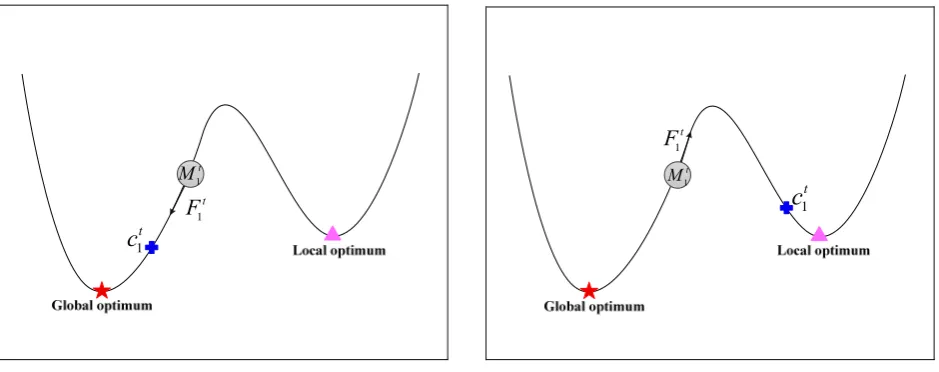
In the original GSA, each agent moves toward the center composed by those elite agents stored in Kbest[32]. If
the center locates at a promising region, the agent’s fitness value becomes increasingly better. As shown in Fig. 1
(a), the center c1t is close to the global optimum and the agent M1t has been self-improved in several sequential
steps in the current iteration t. In this case, the impact of elite masses should be enhanced to strength the movement
tendency of 1
t
M towards the center 1
t
c for accelerating convergence. On the contrary, if the elite masses are
trapped into local optima, especially in the latter stage when the size of Kbest is decreased to a smaller value, their
center is more likely far away from the global optimum. As a result, the agent may experience false convergence
and its fitness can be worse and worse [32,48] as shown in Fig. 1 (b). In this regard, the impact of elite masses
should be weakened to reduce the movement tendency of M1t towards the center c1t for avoiding prematurity.
1
t
c
1
t F
1 t M
1
t
c
1
t F
1
t
M
[image:8.595.68.538.324.510.2](a) Elite agents’ center is close to the global optimum. (b) Elite agents’ center is far away from the global optimum.
Fig. 1. Schematic diagram of the agent’s movement.
As analyzed above, agents may experience different evolutionary states during a course of simulation, which
can be defined in two cases: (1) the agent has improved self-solution in several sequential steps and (2) the agent
has failed to improve self-solution for several sequential steps. The tendency of an agent moving towards elite
masses is supposed to be dynamically changed corresponding to its states for a better convergence. According to Eq.
(6), the gravitational constant Gt is the modulus of force that controls the impact of elite masses. Moreover, by
adjusting the attenuation factor alpha (α), Gt is also changed accordingly. Specifically, a smaller α value results
in a greater Gt that promotes the agent to move faster toward the center of Kbest, while a larger α value leads to a
lower Gt that prevents the agent from reaching the center [9,32]. Therefore, in this paper, the parameter α is
adaptively adjusted according to the agent’s current state.
In order to estimate agents’ evolutionary states, two counters, ns and nf , are used as the indicators. For a
given agent i, the nsti and t i
nf are both set to zero initially. Then, as described in Eqs. (10) and (11), if Xit can
improve self-solution in the new iteration, nsit is incremented by 1 and t i
nf is set to 0. Otherwise, the counter
t i
nf is incremented by 1 whilst nsti is set to 0. Obviously, the values of t i
ns and nfit indicate the different
evolutionary states of the agent i.
1 1
1, 0,
t t t
t i i i
i
ns if fit fit ns otherwise
(10)
1 1
1, 0,
t t t
t i i i
i
nf if fit fit nf otherwise
(11)
We set a limit value lp to judge whether or not to conduct the adjustment of α. For the i-th agent in the
iteration t, if nsit exceeds lp, t i
X is recognized as in the first case [1,49] and its α value should be decreased to
enhance the convergence to elite masses. More specifically, a less variation in fitness or position of agent Xit
denotes its slow movement. Thus, its α value should be decreased greatly to reach a higher convergence speed.
When the position or fitness of agent Xit change greatly, it means the agent moves faster or locates a more
promising region, thus the α value needs be slightly decreased to relatively refine its neighboring areas. On the
other hand, if nfit exceeds lp, t i
X is regarded as in the second case [1,49]. The parameter α is supposed to be
increased to reduce the attraction of elite masses, i.e. its α value changes just in the opposite way as the first case
does. Based on the discussions above, in this paper, the variation of fitness and position of an agent are employed as
feedback to adaptively adjust the parameter α according to the evolutionary state, which is described in Eq. (12).
1 1 1 2 1 1 2 1,..., 1,..., 1 1 2 1 2 1,..., ,exp exp ,
max , max
,
1 exp 1
max ,
t t t t
i i
t i i t
i t t t t i
j j j j
j N j N
t t t
i i t
i
i t t
j j j N
fit fit
α rand if ns lp
ε fit fit ε
α
α + rand
ε X X X X X X X X
1 1 1,..., 1 exp , max , t t t i i i t t j j j N t i fit fitif nf lp fit fit ε
α otherwise (12)
where αit is the alpha value of the i-th agentin the t-th iteration, rand is a random value in [0,1] that can enhance
the diversity of αit [21]. From Eq. (12), it is obvious that t i
α can be dynamically changed in coincidence with its
evolutionary state.
3.2. Stability-based boundary constraint
In GSA, the stability conditions play an important role in promoting the convergence speed and precision. In
this section, after having elaborated investigation of the stability conditions, we present a boundary constraint for
parameter α to enhance the stable convergence of GSA.
As proven in [18], for the i-th agent in the t-th iteration, gravitational constant Gt has to satisfy Eq. (13) to
ensure the stability of its movement trajectory.
4(1 )
,
0 j j i i i j t t t p p
j B j W
w R ε
G M M
where w satisfies the stability condition: 0 w 1, Bi is a set of agents which own better fitness than the agent i,
i
W is a set of agents whose fitness values are no better than the agent i. Mtpj is the personal best fitness history
found so far by the agent j, which is calculated as follows:
1 1 1 1 , , j j
t t t
jd p p
t
jd t t t
jd p p
p if fit fit p
x if fit fit
(14)
j
t t
p t
j t t
fit worst mass
best worst
(15)
1
j
t j t
p N t
k k mass M mass
(16)According to the analysis in [2], parameter α has a drastic influence on Gt. Therefore, on the basis of the
gravitational constant equation in Eq. (6), we can rewrite Eq. (13) as follows:
max max , 0 , 0 0 max , 4(1 ) 0 4(1 ) 0 ln Inf 4(1 ) j j i i j j i i j j i i tα i j
t
t t
p p
j B j W t α i j t t t p p
j B j W
t t
p p
j B j W
i j
w R ε
G e
M M
w R ε
e
G M M
G M M
t
α
t w R ε
(17)where w is set to a certain value in the range
0,1
. For simplicity, we define
min
t
α = max
0 ,
ln j j 4(1 )
i i
t t
p p i j
j B j W
t
G M M w R ε
t
. Eq. (17) offers the lower boundary that α should be
satisfied. Thus, for the agent i in current iteration t, if its alpha value is lower than αmint , αit will be restricted to its
boundary:
min, min
t t t t
i i
Eq. (18) formulates the lower boundary constraint for parameter α. However, there is lack of an upper
boundary constraint for α. In practice, too large value of α can cause the search to the stagnation and impair the
exploration capability. Therefore, it is unreasonable to set the upper boundary value to the infinite great as shown in
Eq. (17). To resolve this problem, we set a parameter αmax to control the upper boundary of α. Note αmax is
fixed to a certain value. In such a way, the boundary constraint equation of α, Eq. (17), can now be rewritten as:
min max
t t
i
α α α (19)
If αit is larger than αmax, it will be conditioned to its upper boundary as follows:
max, max
t t
i i
α α if α α (20)
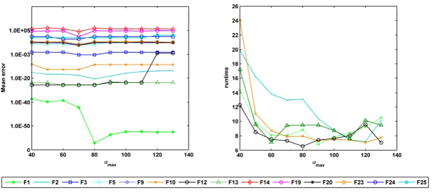
The sensibility tests on αmax in Section 4.4 verify its effectiveness on the performance of GSA. In a word,
the parameter αit should satisfy the boundary conditions as show in Eq. (19). If the t i
α value exceeds its
boundary, αit will be forced to gather on its corresponding boundary as described in Eqs. (18) and (20). Thus,
the stability-based boundary constraint can ensure the stable convergence of the swarm.
Based on the above introduction of the SCAA algorithm, its complete pseudo-code is summarized in
Algorithm 1 as follows.
Algorithm 1 Pseudo-code of SCAA
1 Generate uniformly distributed population randomly and initialize the velocity associated with each agent;
2 Calculate the fitness value of each agent and generate the Kbestagents of the population;
4 While FEs FEs max do
5 /*Adaptive alpha adjusting strategy*/
6 For i1 to NP do
7 If t t1
i i
fit fit
then
8 Set 1
1
t t
i i
ns ns
, nfit0;
9 If nstilp then
10 Set nsit0, decrease
t i
α according to Eq. (12);
11 Else
12 t t1
i i
α α
;
13 End If
14 Else
15 Set 1
1
t t
i i
nf nf
, nsit0;
16 If t i
nf lp then
17 Set nfit0, increase t i
α according to Eq. (12);
18 Else
19 t t1
i i
α α
;
20 End If
21 End If
22 /*Stability-based boundary constraint*/
23 Calculate the lower boundary of alpha min
t
α using Eq. (17);
24 Restrict t i
α to its boundary according to Eqs. (18) and (20);
25 Calculate the acceleration t
i
α by Eqs. (6), (3), (4) and (5);
26 Update the position t
i
X according to Eqs. (7) and (8);
27 Calculate the fitness values t
i
fit ;
28 FEs ;
29 End For
30 t ;
31 End While
3.3. Search behaviors of SCAA
In this section, the search behaviors of SCAA are investigated so as to validate the effectiveness of the proposed
alpha adjusting strategy. We herein take a time-varying 30-D Sphere function as an example.
2
1
, 100,100
D
j j
j
f x r x r x
(21)where r is initialized to -10 and shifted to 10 in the 200th iteration with the total number of iterations set as 2000.
That is, the theoretical minimum of f shifts from (-10)D to (10)D during the evolutionary process. SCAA and GSA
are employed with the same initialized population, which include 50 agents to solve this minimization problem. For
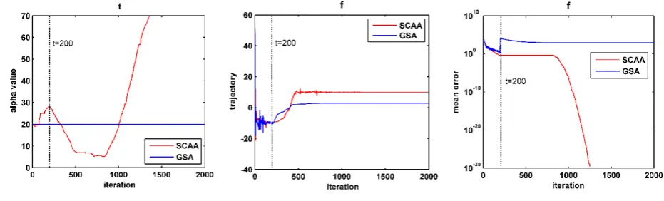
a better observation, only the first agent’s alpha value α1 and its first dimension trajectory x11 are recorded in Fig.
2 (a) and Fig. 2 (b), respectively. The convergence curve of SCAA and GSA are depicted in Fig. 2 (c).
[image:14.595.64.530.460.601.2](a) The curve of α1 values. (b) The trajectory curve of agent x11. (c) The convergence curve.
Fig. 2. Search behaviors of SCAA on 30-D Sphere function.
During the evolutionary process, the center of elite masses is dynamically changed with agents’ movements. In
the early iterations, the elite agents may experience poor areas, hence the center is more likely located at the local
optima. In this case, as shown in Fig. 2 (a), the parameter α1 is continuously increased to a higher value before the
200th iteration to weaken the impact of elite masses. This adjustment prevents the agent from being trapped into
local optima as revealed in Fig. 2 (b). The x11 gradually reaches the global minimum (-10). Thereafter, in the 200th
iteration, the value of r is shifted to 10. At this moment, those agents that are closer to the new global minimum
would be the elite masses in Kbest. To this end, the impact of elite masses should be enhanced to accelerate the
convergence. From the Fig. 2 (b) and Fig. 2(c), it can be seen that parameter α1 is rapidly decreased into a smaller
value whilst the trajectory of x11 deviates from -10 and fast reaches the new global optimum. In the latter
iterations, when agents cluster together and converge to the globally optimal area, less improvement of agents’
fitness are obtained. Therefore, parameter α1 is rapidly increased under the stability-based boundary constraint to
improve the convergence precision. As depicted in Fig. 2 (c), SCAA finally achieves the globally optimal results.
With regard to the original GSA, even though the swarm can converge to the global optimum in the early iterations,
the agents are trapped into local optima after the global minimum is changed. This behavior may mainly result from
the usage of a constant α, which lacks the dynamic momentum in coincidence with the changed search
environment. Conversely, in SCAA, the α value of each agent is adaptively adjusted according to its evolutionary
state, which motivates the agent to detect the promising direction and avoid the premature convergence.
4. Experimental verification and comparison
To fully evaluate the performance of SCAA, a thorough comparison with the original GSA [35] and four recent
GSA variants with well-established alpha adjusting strategies, including MGSA-α [23], FSα(Increase) [43],
FSα(Decrement) [43] and FuzzyGSA [36], is tested in this study. Note that two alpha adjusting methods in [43],
FSα(Increase) and FSα(Decrement), are both introduced for investigating the effect of different alpha change trends
on the searching performance and the stability of GSA. The tested functions include 28 scalable benchmark functions,
where F1-F13 are conventional problems in [54] and F14-F28 are derived from the CEC2015 functions [26]. Detailed
description of these benchmark functions can be found in [26,54]. In this paper, the evaluations are performed under
30 dimensions (30-D) and the accuracy level δ is set to 0.001 for all benchmark functions.
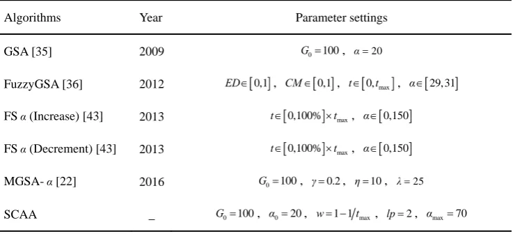
During the experiments, the parameter configurations of all involved algorithms are set according to their
recommended settings [48]. Note that for the fair comparison, MGSA-α only uses the α adjusting strategy and
abandons the mutation operator in MGSA. As for SCAA, the initial value of parameter alpha α0 is set to 20 for all
agents on the basis of the recommendations in [35]. The inertia weight is set to w 1 1tmax according to the range
in stability conditions as suggested in [18]. The limit value lp and αmax are respectively set to 2 and 70 according to
the sensitive analysis conducted in Section 4.5. The detailed parameter settings of all involved algorithms are
summarized in Table 1.
In the experiments, common parameters are the total number of trials, maximum number of function evaluations
(FEsmax) and the population size (NP). All algorithms were independently run 51 times to reduce random discrepancy
[26]. The FEsmax for terminating the algorithms is specified as 10000D for each function as suggested in [26].
The population size NP for solving the 30-D problems is set to 50 based on the recommendation in [35,36,43].
Moreover, since all involved algorithms have the same fitness evaluations FEsNPin each iteration, the maximum
number of iterations tmax is set to tmax FEsmax NP in this paper. All the algorithms are implemented using Matlab
2012b and executed on a computer with Intel Pentium 4 CPU (2.40 GHz) and 4 GB of memory.
[image:17.595.115.484.205.373.2]
Table 1
Parameter settings of the involved GSA variants.
Algorithms Year Parameter settings
GSA [35]
FuzzyGSA [36]
FSα(Increase) [43]
FSα(Decrement) [43]
MGSA-α[22]
SCAA
2009
2012
2013
2013
2016
_
0 100
G , α20
0,1
ED , CM 0,1 , t0,tmax, α29,31
0,100% max
t t , α0,150
0,100% max
t t , α0,150
0 100
G , γ0.2, η10, λ25
0 100
G , α020, w 1 1tmax, lp2, αmax70
4.2. Performance metrics
In this study, the searching accuracy, searching reliability and searching efficiency of different algorithms are
evaluated in terms of the mean error (Mean), success rate (SR), success performance (SP) and execution time
(runtime in seconds), respectively [46]. Mean is the average error between the best output results and the global
optimum of the optimization problem[46]. SR represents the percentage of successful runs where the algorithm
achieves good solutions under the predefined accuracy level δ [46]. SP denotes the number of FEs required by an
algorithm to achieve the acceptable solutions under δ [46]. The performance metric runtime is the execution time of
an algorithm to obtain the acceptable solutions [27]. Meanwhile, we record the standard deviation (SD) of the
optimization error and rank the algorithms from the smallest Mean to the highest. The average ranks and the overall
ranks obtained by algorithms are also recorded.
For the rigorous comparison between SCAA and its competitors, a non-parametric statistical test is used in this
study. Unlike parametric tests, non-parametric tests are employed to analyze the performance of stochastic algorithms
based on computational intelligence despite the assumptions of data types used are violated [10]. Specifically, the
Wilcoxon signed ranks test [6] with a confidence level of 5% is utilized to perform pairwise comparison between
SCAA and its peers in this paper.
4.3. Comparison with other alpha adjusting GSA variants
Following the experimental setup and parameter settings in Section 4.1, comprehensive experiments are employed
to evaluate the overall searching behaviors of GSA, MGSA-α, FuzzyGSA, FSα(Increase), FSα(Decrement) and
SCAA. For performance assessment, six metrics are used which include the Mean, SD and Wilcoxon signed ranks
test (p-value, h-value, z-value and signedrank), as summarized in Table 2 and Table 3, along with SR, SP and runtime
as reported in Table 4. Besides, we rank the six competing algorithms according to their Mean values. In Table 2 and
Table 3, the symbol ‘h’ describes the non-parameter test results, where ‘+’ means SCAA is significantly better than
the compared algorithms, ‘-’ indicates it significantly performs worse and ‘=’ stands for comparable performance
between the algorithms. Moreover, we summarize the results of Wilcoxon test results at the bottom of Table 2 and
Table 3, respectively. The best result in each row is highlighted in bold in the Tables 2-4. Note that Fig. 3 depicts some
convergence curves of the competing algorithms.
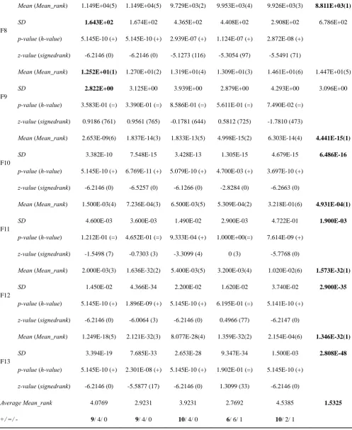
Table 2
metrics GSA MGSA-α FuzzyGSA FSα(Increase) FSα(Decrement) SCAA
F1
Mean (Mean_rank) 1.188E-17(6) 4.481E-34(3) 7.291E-27(5) 1.322E-38(2) 6.514E-27(4) 9.162E-58(1)
SD 3.398E-18 7.093E-34 2.081E-27 4.230E-38 7.117E-28 2.283E-57
p-value (h-value) 5.145E-10 (+) 5.145E-10 (+) 5.145E-10 (+) 5.145E-10 (+) 5.145E-10 (+) z-value (signedrank) -6.2146 (0) -6.2146 (0) -6.2146 (0) -6.2146 (0) -6.2146 (0)
F2
Mean (Mean_rank) 1.727E-08(6) 3.038E-16(3) 4.257E-13(5) 1.247E-18(2) 3.855E-13(4) 4.558E-20(1)
SD 2.829E-09 2.295E-16 5.629E-14 1.094E-18 1.52E-15 9.218E-20
p-value (h-value) 5.145E-10 (+) 5.145E-10 (+) 5.145E-10 (+) 9.662E-09 (+) 5.145E-10 (+) z-value (signedrank) -6.2146 (0) -6.2146 (0) -6.2146 (0) -5.7366 (51) -6.2146 (0)
F3
Mean (Mean_rank) 1.500E-02(2) 2.264E+00(3) 1.272E+01(4) 5.556E+01(5) 1.749E+02(6) 7.700E-03(1)
SD 3.010E-02 2.207E+00 7.251E+00 2.557E+01 6.488E+01 5.600E-03
p-value (h-value) 1.197E-01 (=) 5.145E-10 (+) 5.145E-10 (+) 5.145E-10 (+) 5.145E-10 (+) z-value (signedrank) -1.5560 (497) -6.2146 (0) -6.2146 (0) -6.2146 (0) -6.2146 (0)
F4
Mean (Mean_rank) 1.823E-09(6) 5.247E-16(2) 5.486E-14(5) 1.329E-18(1) 3.385E-14(3) 5.041E-14(4)
SD 2.171E-10 2.276E-16 9.236E-15 6.262E-19 2.305E-15 2.008E-13
p-value (h-value) 5.145E-10 (+) 9.104E-01 (=) 1.309E-05 (+) 1.768E-09 (-) 1.309E-05 (-) z-value (signedrank) -6.2146 (0) 0.1125 (675) -4.3587 (198) 6.0178 (1305) -4.3587 (198)
F5
Mean (Mean_rank) 1.918E+01(2) 2.214E+01(3) 2.387E+01(4) 2.901E+01(5) 3.223E+01(6) 1.321E+01(1)
SD 2.264E-01 1.769E-01 1.743E-01 2.290E+01 3.235E+01 4.512E-01
p-value (h-value) 5.145E-10 (+) 5.145E-10 (+) 5.145E-10 (+) 5.145E-10 (+) 5.145E-10 (+) z-value (signedrank) -6.2146 (0) -6.2146 (0) -6.2146 (0) -6.2146 (0) -6.2146 (0)
F6
Mean (Mean_rank) 0.00E+00(1) 0.00E+00(1) 0.00E+00(1) 0.00E+00(1) 0.00E+00(1) 0.00E+00(1) SD 0.00E+00 0.00E+00 0.00E+00 0.00E+00 0.00E+00 0.00E+00 p-value (h-value) 1.000E+00(=) 1.000E+00(=) 1.000E+00(=) 1.000E+00(=) 1.000E+00(=) z-value (signedrank) — (0) — (0) — (0) — (0) — (0)
F7
Mean (Mean_rank) 9.24E-02(6) 8.18E-02(5) 1.070E-02(2) 1.240E-02(3) 1.460E-02(4) 1.050E-02(1)
SD 3.560E-02 2.890E-02 3.200E-03 5.000E-03 5.200E-03 6.200E-03
F8
Mean (Mean_rank) 1.149E+04(5) 1.149E+04(5) 9.729E+03(2) 9.953E+03(4) 9.926E+03(3) 8.811E+03(1) SD 1.643E+02 1.674E+02 4.365E+02 4.408E+02 2.908E+02 6.786E+02 p-value (h-value) 5.145E-10 (+) 5.145E-10 (+) 2.939E-07 (+) 1.124E-07 (+) 2.872E-08 (+)
z-value (signedrank) -6.2146 (0) -6.2146 (0) -5.1273 (116) -5.3054 (97) -5.5491 (71)
F9
Mean (Mean_rank) 1.252E+01(1) 1.270E+01(2) 1.319E+01(4) 1.309E+01(3) 1.461E+01(6) 1.447E+01(5) SD 2.822E+00 3.125E+00 3.939E+00 2.879E+00 4.293E+00 3.096E+00 p-value (h-value) 3.583E-01 (=) 3.390E-01 (=) 8.586E-01 (=) 5.611E-01 (=) 7.490E-02 (=)
z-value (signedrank) 0.9186 (761) 0.9561 (765) -0.1781 (644) 0.5812 (725) -1.7810 (473)
F10
Mean (Mean_rank) 2.653E-09(6) 1.837E-14(3) 1.833E-13(5) 4.998E-15(2) 6.303E-14(4) 4.441E-15(1)
SD 3.382E-10 7.548E-15 3.428E-13 1.305E-15 4.679E-15 6.486E-16
p-value (h-value) 5.145E-10 (+) 6.769E-11 (+) 5.079E-10 (+) 4.700E-03 (+) 3.697E-10 (+) z-value (signedrank) -6.2146 (0) -6.5257 (0) -6.1266 (0) -2.8284 (0) -6.2663 (0)
F11
Mean (Mean_rank) 1.500E-03(4) 7.236E-04(3) 6.500E-03(5) 5.309E-04(2) 3.218E-01(6) 4.931E-04(1)
SD 4.600E-03 3.600E-03 1.490E-02 2.900E-03 4.722E-01 1.900E-03
p-value (h-value) 1.212E-01 (=) 4.652E-01 (=) 9.333E-04 (+) 1.000E+00(=) 7.614E-09 (+) z-value (signedrank) -1.5498 (7) -0.7303 (3) -3.3099 (4) 0 (3) -5.7768 (0)
F12
Mean (Mean_rank) 2.000E-03(3) 1.636E-32(2) 5.400E-03(5) 3.200E-03(4) 1.020E-02(6) 1.573E-32(1)
SD 1.450E-02 4.366E-34 2.200E-02 1.620E-02 3.740E-02 2.900E-35
p-value (h-value) 5.145E-10 (+) 1.896E-09 (+) 5.145E-10 (+) 6.195E-01 (=) 5.141E-10 (+) z-value (signedrank) -6.2146 (0) -6.0064 (3) -6.2146 (0) 0.4966 (77) -6.2147 (0)
F13
Mean (Mean_rank) 1.249E-18(5) 2.121E-32(3) 8.077E-28(4) 1.359E-32(2) 2.154E-04(6) 1.346E-32(1)
SD 3.394E-19 7.685E-33 2.653E-28 9.347E-34 1.500E-03 2.808E-48
p-value (h-value) 5.145E-10 (+) 2.301E-08 (+) 5.145E-10 (+) 1.902E-01 (=) 5.145E-10 (+) z-value (signedrank) -6.2146 (0) -5.5877 (17) -6.2146 (0) 1.3099 (33) -6.2146 (0)
Average Mean_rank 4.0769 2.9231 3.9231 2.7692 4.5385 1.5325
[image:20.595.49.547.76.684.2]+/ =/ - 9/ 4/ 0 9/ 4/ 0 10/ 4/ 0 6/ 6/ 1 10/ 2/ 1
Table 3
metrics GSA MGSA-α FuzzyGSA FSα(Increase) FSα(Decrement) SCAA
F14
Mean (Mean_rank) 8.737E+05(2) 1.012E+06(3) 2.707E+06(5) 2.046E+06(4) 1.428E+07(6) 4.093E+05(1)
SD 4.497E+05 3.907E+05 5.063E+06 1.297E+06 8.813E+06 2.405E+05
p-value (h-value) 1.273E-08 (+) 9.141E-09 (+) 4.673E-09 (+) 5.145E-10 (+) 5.145E-10 (+) z-value (signedrank) -5.6897 (56) -5.7459 (50) -5.5884 (38) -6.2146 (0) -6.2146 (0)
F15
Mean (Mean_rank) 4.729E+02(2) 7.445E+02(5) 7.169E+02(4) 7.634E+02(6) 4.701E+02(1) 5.328E+02(3) SD 4.771E+02 9.367E+02 9.480E+02 1.117E+03 6.262E+02 8.585E+02 p-value (h-value) 5.486E-01 (=) 3.250E-01 (=) 2.489E-01 (=) 2.528E-01 (=) 7.858E-01 (=)
z-value (signedrank) -0.5999 (599) -0.9842 (558) -1.1529 (540) -1.1436 (541) -0.2718 (634)
F16
Mean (Mean_rank) 2.00E+01(1) 2.00E+01(1) 2.00E+01(1) 2.00E+01(1) 2.00E+01(1) 2.094E+01(2)
SD 9.746E-05 6.594E-05 8.113E-05 1.109E-04 6.150E-05 5.840E-02
p-value (h-value) 5.145E-10 (-) 5.145E-10 (-) 5.145E-10 (-) 5.145E-10 (-) 5.145E-10 (-) z-value (signedrank) 6.2146 (1326) 6.2146 (1326) 6.2146 (1326) 6.2146 (1326) 6.2146 (1326)
F17
Mean (Mean_rank) 2.073E+02(2) 1.963E+02(1) 2.194E+02(5) 2.084E+02(3) 2.363E+02(6) 2.173E+02(4)
SD 2.201E+01 2.811E+01 1.924E+01 2.023E+01 2.261E+01 2.223E+01
p-value (h-value) 2.830E-02 (+) 5.617E-04 (-) 4.148E-01 (=) 4.900E-03 (+) 1.215E-04 (+) z-value (signedrank) -2.1934 (429) -3.4494 (295) -0.8155 (576) -2.8120 (363) -3.8431 (253)
F18
Mean (Mean_rank) 3.818E+03(4) 3.625E+03(1) 3.981E+03(5) 3.773E+03(2) 4.156E+03(6) 3.810E+03(3)
SD 4.518E+02 4.456E+02 4.533E+02 5.325E+02 4.548E+02 4.548E+02
p-value (h-value) 7.930E-01 (=) 2.010E-02 (-) 7.190E-02 (=) 9.030E-01 (=) 7.916E-04 (+) z-value (signedrank) -0.2625 (635) -2.3246 (415) -1.7997 (471) -0.1219 (650) -3.3557 (305)
F19
Mean (Mean_rank) 1.302E+05(2) 3.553E+05(3) 6.856E+05(4) 9.472E+05(5) 1.704E+06(6) 5.587E+04(1)
SD 6.396E+04 1.725E+05 2.962E+05 3.593E+05 6.204E+05 2.566E+04
p-value (h-value) 1.420E-08 (+) 5.145E-10 (+) 5.145E-10 (+) 5.145E-10 (+) 5.145E-10 (+) z-value (signedrank) -5.6709 (58) -6.2146 (0) -6.2146 (0) -6.2146 (0) -6.2146 (0)
F20
Mean (Mean_rank) 1.324E+01(2) 1.524E+01(3) 2.236E+01(4) 2.441E+01(5) 6.397E+01(6) 9.779E+00(1)
SD 4.061E+00 9.643E+00 1.949E+01 2.058E+01 2.388E+01 3.133E+00
F21
Mean (Mean_rank) 2.356E+04(2) 2.388E+04(3) 3.050E+04(4) 5.557E+04(5) 1.007E+05(6) 2.154E+04(1)
SD 1.079E+04 7.509E+03 1.152E+04 3.344E+04 1.141E+05 8.329E+03
p-value (h-value) 2.728E-01 (=) 6.760E-02 (=) 1.201E-06 (+) 5.797E-10 (+) 5.145E-10 (+) z-value (signedrank) -1.0967 (546) -1.8278 (468) -4.8555 (145) -6.1959 (2) -6.2146 (0)
F22
Mean (Mean_rank) 1.511E+02(4) 1.265E+02(2) 1.513E+02(5) 1.262E+02(1) 2.025E+02(6) 1.358E+02(3)
SD 1.218E+02 8.221E+01 1.218E+02 7.943E+01 1.627E+02 1.016E+02
p-value (h-value) 1.700E-03 (+) 6.080E-02 (=) 7.446E-06 (+) 1.469E-04 (-) 1.425E-05 (+) z-value (signedrank) -3.1307 (329) -1.8747 (463) -4.4805 (185) -3.7963 (258) -4.3399 (200)
F23
Mean (Mean_rank) 4.299E+05(2) 6.936E+05(3) 9.961E+0545) 1.280E+06(5) 2.485E+06(6) 1.921E+05(1)
SD 1.961E+05 2.310E+05 3.994E+05 6.108E+05 1.004E+06 5.998E+04
p-value (h-value) 9.869E-10 (+) 5.145E-10 (+) 5.145E-10 (+) 5.462E-10 (-) 5.145E-10 (+) z-value (signedrank) -6.115 (11) -6.2146 (0) -6.2146 (0) -6.2052 (1) -6.2146 (0)
F24
Mean (Mean_rank) 3.244E+02(2) 3.343E+02(3) 3.480E+02(5) 3.473E+02(4) 3.849E+02(6) 3.226E+02(1)
SD 9.771E+01 1.121E+02 1.557E+02 1.422E+02 2.021E+02 9.132E+01
p-value (h-value) 6.080E-02 (=) 6.675E-04 (+) 1.272E-08 (+) 8.648E-09 (+) 8.648E-09 (+) z-value (signedrank) -1.8747 (463) -3.4026 (300) -5.6897 (56) -5.7553 (49) -5.7553 (49)
F25
Mean (Mean_rank) 1.040E+02(3) 1.036E+02(2) 1.053E+02(5) 1.047E+02(4) 1.491E+02(6) 1.034E+02(1)
SD 8.472E-01 8.215E-01 1.104E+00 9.304E-01 2.771E+01 7.031E-01
p-value (h-value) 2.473E-04 (+) 2.302E-01 (=) 1.873E-09 (+) 2.070E-07 (+) 5.145E-10 (+) z-value (signedrank) -3.6650 (272) -1.1998 (535) -6.0084 (22) -5.1929 (109) -6.2146 (0)
F26
Mean (Mean_rank) 5.527E+03(6) 4.759E+03(5) 1.673E+03(3) 1.602E+03(2) 2.100E+03(4) 1.550E+03(1)
SD 3.988E+03 3.987E+03 1.083E+03 1.571E+03 1.121E+03 1.296E+03
p-value (h-value) 2.905E-06 (+) 1.425E-05 (+) 6.528E-01 (=) 6.528E-01 (=) 2.220E-02 (+) z-value (signedrank) -4.6774 (164) -4.3399 (200) -0.4499 (615) 0.4499 (711) -2.2871 (419)
F27
Mean (Mean_rank) 1.00E+02(1) 1.00E+02(1) 1.00E+02(1) 1.00E+02(1) 2.821E+04(2) 1.00E+02(1)
SD 1.385E-07 8.716E-13 6.668E-10 0.00E+00 7.551E+03 3.565E-13
p-value (h-value) 5.145E-10 (+) 6.380E-02 (=) 5.145E-10 (+) 1.573E-01 (=) 5.145E-10 (+) z-value (signedrank) -6.2146 (0) -1.8537 (10) -6.2146 (0) -1.4142 (0) -6.2146 (0)
SD 1.712E-10 4.295E-13 2.422E-10 1.435E-13 7.414E+00 1.435E-13
p-value (h-value) 5.139E-10 (+) 2.034E-07 (+) 5.127E-10 (+) 1.000E+00 (=) 5.145E-10 (+) z-value (signedrank) -6.2148 (0) -5.1962 (0) -6.2152 (0) — (0) -6.2146 (0)
Average Mean_rank 2.4667 2.5333 3.8000 3.0000 4.6667 1.7333
+/ =/ - 10/ 4/ 0 7/ 5/ 3 10/ 4/ 2 7/ 5/ 3 13/ 1/ 1
Searching accuracy:
From Table 2 and Table 3, we can conclude that SCAA performs the best searching accuracy as it
outperforms its peers with a large margin in most of the problems. SCAA exhibits 11 best Mean values out of
13 for conventional problems (Table 2) and obtains 10 best Mean values out of 15 for CEC2015 functions
(Table 3). Specifically, for the conventional problems, SCAA ranks the first on 5 multimodal problems (F8,
F10-F13). These functions have multiple local optima around the global optimum, which can mislead the
swarm into the non-optimal basin. While in SCAA, thanks to the proposed dynamic α adjustment strategy, it
has successfully enabled the population to track more promising regions and realize the balance between
exploration and exploitation on multimodal functions.
As for the CEC2015 functions, it is noticeable that all involved algorithms suffer from performance
degradation and none of them can find the acceptable solutions. Even so, SCAA achieves most number of best
Mean values compared with other algorithms. To be specific, the performance of SCAA is superior on the
unimodal functions (F14 and F15), hybrid functions (F19-F21) and composition functions (F22-F28). However,
SCAA performs mediocrely on the multimodal functions (F16-F18) in which SCAA ranks 2th, 4th and 3th out of
6 algorithms on F16, F17 and F18, respectively. These functions possess a huge number of local optima [26]
that are more complex than the conventional multimodal functions. The mediocre performance of SCAA may come
from its α boundary constraint, which may block agents’ jumping-out momentum to explore the whole search
space. Therefore, this limitation can be further explored in the future work.
According to the statistic results in the last row of Table 2 and Table 3, the involved algorithms obtain different
rank values on conventional problems and CEC2015 functions, which validate their distinguishing search
performance. Nevertheless, SCAA has the minimum value in Average rank and obtains the first place of results in
both tables, which confirm the superior searching accuracy of SCAA. In addition, SCAA performs relatively robust
towards the 28 benchmark functions as evidenced by its smallest SD values.
Wilcoxon signed ranks test:
From Tables 2 and 3, it is apparent that SCAA has significant better performance compared to its peers in most
cases. For the conventional problems, SCAA are significantly better than GSA, MGSA-α, FuzzyGSA,
FSα(Increase) and FSα(Decrement) on 9, 9, 10, 6 and 10 functions, respectively. FSα(Increase) and
FSα(Decrement) are statistically better than SCAA only on one function (F4), while GSA, MGSA-α and
FuzzyGSA cannot statistically outperform SCAA on any conventional functions. As for the CEC2015 functions,
when compared with GSA, MGSA-α , FuzzyGSA, FSα(Increase) and FSα(Decrement), SCAA shows
significantly better performance on 10, 7, 10, 7 and 13 functions and exhibits statistically worse performance just
on 1, 3, 2, 3 and 1 functions, respectively. These statistic results have validated the competitive advantages of the
proposed SCAA approach.
Table 4
Convergence speed and reliability comparison among six algorithms on conventional functions at 30-D.
metrics GSA MGSA-α FuzzyGSA FSα(Increase) FSα(Decrement) SCAA
F1
SP (SR%) 8.03E+04 (100) 6.93E+04 (100) 5.64E+04 (100) 4.43E+04 (100) 2.47E+04 (100) 2.41E+04 (100)
runtime 14.8011 12.7453 17.4103 10.8446 7.1359 6.6472
F2
SP (SR%) 1.52E+05 (100) 1.24E+05 (100) 1.03E+05 (100) 7.16E+04 (100) 5.14E+04 (100) 3.90E+04 (100)
runtime 30.5721 24.3482 34.4027 18.1258 13.3601 12.3655
F3
SP (SR%) 8.65E+04 (33.3) Inf (0) Inf (0) Inf (0) Inf (0) Inf (0)
runtime 38.1149 Inf Inf Inf Inf Inf
F4
SP (SR%) 1.18E+05 (100) 9.79E+04 (100) 8.17E+04 (100) 5.88E+04 (100) 3.80E+04 (100) 7.96E+04 (100)
runtime 23.2371 18.2716 25.4612 14.6428 9.6580 20.3386
F5
SP (SR%) Inf (0) Inf (0) Inf (0) Inf (0) Inf (0) Inf (0)
runtime Inf Inf Inf Inf Inf Inf
F6
SP (SR%) 2.65E+04 (100) 2.88E+04 (100) 1.79E+04 (100) 1.94E+04 (100) 1.56E+04 (100) 1.09E+04 (100)
runtime 4.9064 5.0853 26.0255 4.7630 1.7719 3.0915
F7
SP (SR%) Inf (0) Inf (0) Inf (0) Inf (0) Inf (0) Inf (0)
runtime Inf Inf Inf Inf Inf Inf
F8
SP (SR%) Inf (0) Inf (0) Inf (0) Inf (0) Inf (0) Inf (0)
runtime Inf Inf Inf Inf Inf Inf
F9
SP (SR%) Inf (0) Inf (0) Inf (0) Inf (0) Inf (0) Inf (0)
runtime Inf Inf Inf Inf Inf Inf
F10
SP (SR%) 1.28E+05 (100) 1.04E+05 (100) 8.65E+04 (100) 6.12E+04 (100) 4.11E+04 (100) 3.84E+04 (100)
runtime 25.5664 20.7946 28.3058 15.4832 10.9001 9.8405
F11
SP (SR%) 5.77E+04 (100) 5.24E+04 (100) 4.04E+04 (100) 3.49E+04 (100) Inf (0) 3.51E+04 (100)
runtime 11.4403 10.2226 22.7925 9.0093 Inf 13.2134
F12
SP (SR%) 4.51E+04 (100) 4.19E+04 (100) 3.12E+04 (100) 2.89E+04 (100) 1.07E+04 (100) 2.94E+04 (100)
runtime 13.2818 11.9072 16.0448 10.7113 3.8040 7.4324
F13
SP (SR%) 6.62E+04 (100) 5.65E+04 (100) 4.32E+04 (100) 3.83E+04 (100) 2.01E+04 (100) 1.38E+04 (100)
runtime 14.8885 12.6030 15.3931 10.9785 5.8154 9.8506
Average runtime 19.6454 14.4905 23.2295 11.8198 7.4923 10.3474
Convergence comparison:
The speed in obtaining an acceptable solution is also a salient yardstick for measuring the performance of an
algorithm. For testing the searching efficiency of SCAA, the metric SP, runtime and convergence curves are also
reported for comparison. It is worth mentioning that if one algorithm cannot solve the problem (SR=0%), the SP
value is defined as infinity (Inf). Because of the strict threshold settings, none of the involved algorithms can
achieve the available SP values on all CEC2015 functions. Thus, only the results on 13 conventional functions are
recorded. As shown in Table 4, SCAA achieves the smallest SP values on 5 conventional problems (F1, F2, F6, F10
and F13), which is obviously better than that of its 5 peers. The fast convergence characteristic of SCAA mainly
results from its adaptive adjustment of the parameter alpha.
As for the runtime results, SCAA has a tendency to spend slightly more computational time due to its repeating
calculation of the ratio of mass and distance between any two agents in the stability conditions in each iteration.
Nevertheless, from Table 4 we can conclude that SCAA spends the least computational time on unimodal functions
F1 and F2. These results may benefit from the superior SP results of SCAA, which can decrease its runtime values
to some extent. For more complicated functions, superiority on efficiency of SCAA is not as obvious as that on F1
and F2. This is mainly because that the global optimum in these functions can be very far away from the local
optima or can be surrounded by a considerable amount of local optima [4]. In this situation, for avoiding trapping
into the local optima, the parameter alpha in SCAA is adjusted to decrease the convergence tendency of agents to
the elite masses, which causes the increase of execution time. Even so, the average runtime of SCAA ranks the
second among the competing algorithms as listed at the bottom of Table 4. In this experiment, FSα(Decrement)
ranks the first according to its average runtime. This is primarily because the decreasing trend of α from an initial
value 150 enables FSα(Decrement) to have a much larger α value during the whole iteration, which can improve
the convergence speed. However, the larger alpha value can lead to the smaller search steps of agents and easily
cause the premature convergence. This is observed by the poor searching performance of FSα(Decrement) as
shown in Table 2 of the manuscript.
A closer look at the convergence curves of different algorithms in Fig. 3 provides more insight into their
searching behavior. The figure includes the representative conventional problems (F1, F2, F3, F5, F10 and F13) and
CEC2015 functions (F14, F19, F20, F21, F23 and F24). Based on the graphical results in Fig. 3, the outstanding
convergence characteristics of SCAA on different test functions are explained. Specifically, for the conventional
problems, the convergence curves of SCAA sharply drop at one point on functionsF1, F2, F3, F5, F10 and F13 in
the early iterations and then reach better results in the latter iterations. These observations prove the capability of
SCAA to facilitate the balance between exploration and exploitation. With regard to the CEC2015 functions,
because of their complex characteristics, the convergence speeds of all involved algorithms are slightly inferior to
that in conventional problems. Nevertheless, the convergence curves of SCAA rapidly drop at one point on
functions F14, F19, F23 and F24 in the early iterations. On functions F20 and F21, the convergence speed of SCAA
is more slowly than its peers at the early stage, while its speed increases in the middle stage of optimization.
Moreover, SCAA achieves superior convergence accuracy among all algorithms, which may result from the ability
of α boundary constraint to improve convergence precision in the latter iterations. In general, SCAA has produced
improved searching efficiency compared with other algorithms.
Fig. 3. Convergence curves of different alpha adjusting GSA variants.
4.4. Stability analysis of SCAA
In order to validate the stability of SCAA, the trajectories of agents are analyzed. Experiments are conducted on
three conventional functions F2, F7 and F9, respectively. For a better observation, the number of iterations is set to
100 and the trajectory of the first dimension for the first agent, denoted as x11 in each algorithm, is recorded.
Experiments are carried out with 51 independent runs and the average trajectory curves are listed in Fig. 4. Note
that the stability stage occurs when there is little variation in an agent’s position between iterations [8,18].
First, in order to analyze the effect of stability boundary constraint, we compare the performance of SCAA in
two cases: SCAA with stability constraints and SCAA without stability constraints (denoted as SCAA-Ns). From
the trajectory curves in Fig. 4 (a)-(c), it is clear that the agent’s trajectory in red line (SCAA) are more stable than
that in blue line (SCAA-Ns), which validates that the stability constraints play an important role in guaranteeing the
stable convergence.
Second, we make the stability comparison between SCAA and other involved algorithms. The results are
plotted in Fig. 4 (d)-(f). It can be observed that SCAA performs more stable when compared with other algorithms.
To be specific, the agent trajectories of GSA, FSα(Increase) and MGSA-α are rather unstable, whereas SCAA
and FSα(Decrement) are more stable. Particularly, the agent trajectories of FSα(Decrement) is more stable than
that in SCAA. This may because that the decreasing trend of α from an initial value 150 in FSα(Decrement)