Smart TSO-DSO interaction schemes, market architectures and ICT Solutions for the integration of ancillary services from demand side management and distributed generation
SmartNet simulation platform
Authors:
Giacomo Viganò, Marco Rossi (RSE), Peter Sels, Guillaume Leclercq, Thomas Gueuning, Marco Pavesi (N-SIDE), Yelena Vardanyan, Razgar Ebrahimy (DTU), Joseba Jimeno, Nerea Ruiz (TECNALIA), Gary Howorth (USTRATH), Juliano Camargo, Chris Hermans, Fred Spiessen (VITO), Harald Svendsen (SINTEF),
Distribution Level Public
Responsible Partner RSE
Checked by WP leader Marco Rossi
Date: 21/06/2019
Approved by Project Coordinator
Gianluigi Migliavacca
Date: 25/06/2019
Issue Record
Planned delivery date M36 (31/12/2018) Actual date of delivery M42 (30/06/2019) Status and version 1.0 – Final
Version Date Author(s) Notes
0.0 October 2018 RSE First template with description of physical layer 0.5 November 2018 N-SIDE, DTU,
TECNALIA, USTRATH, VITO, SINTEF
Contributions received by partners
0.7 May 2019 RSE Harmonization of the content
0.8 June 2019 N-DISE, DTU,
TECNALIA, USTRATH, VITO, SINTEF
Revision of the content
0.9 June 2019 RSE Revision by WP leader
Copyright 2019 SmartNet Page 1
About SmartNet
The project SmartNet (http://smartnet-project.eu) aims at providing architectures for optimized interaction between TSOs and DSOs in managing the exchange of information for monitoring, acquiring and operating ancillary services (frequency control, frequency restoration, congestion management and voltage regulation) both at local and national level, taking into account the European context. Local needs for ancillary services in distribution systems should be able to co-exist with system needs for balancing and congestion management. Resources located in distribution systems, like demand side management and distributed generation, are supposed to participate to the provision of ancillary services both locally and for the entire power system in the context of competitive ancillary services markets.
Within SmartNet, answers are sought for to the following questions:
• Which ancillary services could be provided from distribution grid level to the whole power system?
• How should the coordination between TSOs and DSOs be organized to optimize the processes of procurement and activation of flexibility by system operators?
• How should the architectures of the real time markets (in particular the markets for frequency restoration and congestion management) be consequently revised?
• What information has to be exchanged between system operators and how should the communication (ICT) be organized to guarantee observability and control of distributed generation, flexible demand and storage systems? The objective is to develop an ad hoc simulation platform able to model physical network, market and ICT in order to analyse three national cases (Italy, Denmark, Spain). Different TSO-DSO coordination schemes are compared with reference to three selected national cases (Italian, Danish, Spanish).
The simulation platform is then scaled up to a full replica lab, where the performance of real controller devices is tested. In addition, three physical pilots are developed for the same national cases testing specific technological solutions regarding:
• monitoring of generators in distribution networks while enabling them to participate to frequency and voltage regulation,
• capability of flexible demand to provide ancillary services for the system (thermal inertia of indoor swimming pools, distributed storage of base stations for telecommunication).
Copyright 2019 SmartNet Page 2
Table of Contents
1 The SmartNet Simulator ... 9
1.1 Time axis of the simulation ... 10
1.1.1 Aggregation/Market/Disaggregation Latency (from devices data collection to application of set-points) ... 13
1.1.2 Market clearing frequency ... 14
1.1.3 Pipelining ... 15
1.2 Simulation of the SmartNet TSO-DSO coordination schemes ... 17
1.2.1 TSO-DSO coordination scheme A – Centralized ancillary services market model ... 18
1.2.2 TSO-DSO coordination scheme B – Local ancillary services market model ... 19
1.2.3 TSO-DSO coordination scheme C – Shared balancing responsibility model ... 20
1.2.4 TSO-DSO Coordination scheme D – Common TSO-DSO ancillary services market model21 1.2.5 Process describing the independent evolution of device status and network ... 22
2 Scheduler ... 24
2.1 Brief description of the module ... 24
2.2 The high level architecture ... 24
2.3 Input from database ... 26
2.4 List of functions of the module ... 26
2.5 Output to database ... 27
3 Bidding and dispatching layer ... 28
3.1 Atomic Loads Aggregation/Disaggregation module ... 29
3.1.1 Brief description of the module ... 29
3.1.2 Input from other modules ... 30
3.1.3 Flow chart of the module ... 31
3.1.4 Output to database ... 34
3.2 TCL Aggregation module ... 35
3.2.1 Brief description of the module ... 35
3.2.2 Input from database ... 36
3.2.3 Input from other modules ... 37
3.2.4 List of functions of the module ... 37
3.2.5 Flow chart of the module ... 39
3.2.6 Output to database ... 42
3.3 TCL Disaggregation module ... 44
3.3.1 Brief description of the module ... 44
3.3.2 Input from database ... 44
Copyright 2019 SmartNet Page 3
3.3.4 List of functions of the module ... 45
3.3.5 Flow chart of the module ... 45
3.3.6 Output to database ... 46
3.4 Conventional Generators Aggregation module ... 47
3.4.1 Brief description of the module ... 47
3.4.2 Input from database ... 47
3.4.3 Input from other modules ... 48
3.4.4 List of functions of the module ... 48
3.4.5 Flow chart of the module ... 48
3.4.6 Output to database ... 50
3.5 Conventional Generators Disaggregation module ... 51
3.5.1 Brief description of the module ... 51
3.5.2 Input from database ... 51
3.5.3 Input from other modules ... 51
3.5.4 List of functions of the module ... 52
3.5.5 Flow chart of the module ... 52
3.5.6 Output to database ... 53
3.6 CHP Aggregation module ... 54
3.6.1 Brief description of the module ... 54
3.6.2 Input from database ... 54
3.6.3 Input from other modules ... 55
3.6.4 List of functions of the module ... 55
3.6.5 Flow chart of the module ... 55
3.6.6 Output to database ... 57
3.7 CHP Disaggregation module ... 58
3.7.1 Brief description of the module ... 58
3.7.2 Input from database ... 58
3.7.3 Input from other modules ... 58
3.7.4 List of functions of the module ... 58
3.7.5 Flow chart of the module ... 59
3.7.6 Output to database ... 60
3.8 Curtailable generation and curtailable load Aggregration/Disaggregation module ... 61
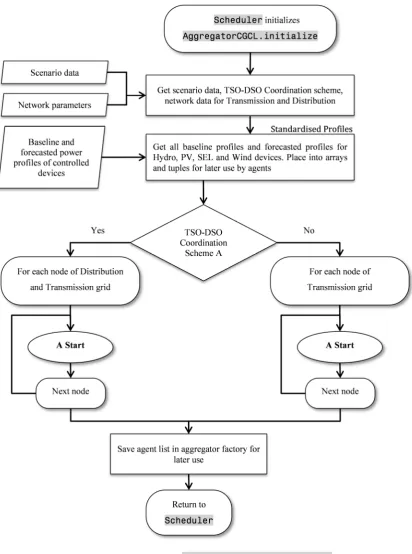
3.8.1 Brief description of the module ... 61
3.8.1.1 CGCL Aggregator Factory... 62
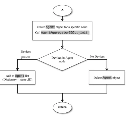
3.8.1.2 CGCL Aggregator Implementation Module (Agent Logic)... 63
3.8.2 Input from database ... 65
Copyright 2019 SmartNet Page 4
3.8.3.1 Inputs for CGCL Aggregator Factory ... 67
3.8.3.2 Inputs for CGCL aggregator implementation ... 67
3.8.4 Flow chart of the module ... 68
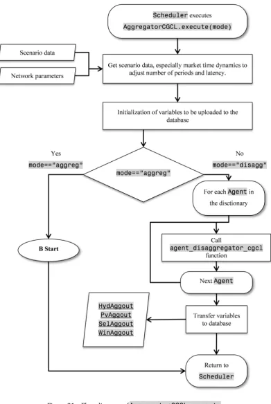
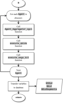
3.8.4.1 CGCL Aggregator Factory Module ... 68
3.8.4.2 CGCL Aggregator Implementation Module ... 74
3.8.5 Output to database ... 77
3.8.5.1 Aggregation Bids to Market ... 77
3.8.5.2 Disaggregation Outputs ... 77
3.9 Electrical Energy Storage unit aggregation module ... 79
3.9.1 Brief description of the module ... 79
3.9.2 Input from database ... 79
3.9.3 Input from other modules ... 80
3.9.4 List of functions of the module ... 81
3.9.5 Flow chart of the module ... 82
3.9.6 Output to database ... 82
3.10 Electrical Energy Storage unit disaggregation module ... 84
3.10.1 Brief description of the module ... 84
3.10.2 Input from database... 84
3.10.3 Input from other modules ... 85
3.10.4 List of functions of the module ... 85
3.10.5 Flow chart of the module ... 85
3.10.6 Output to database ... 86
4 Market layer ... 87
4.1 Brief description of the module and flowchart ... 87
4.2 Inputs from database ... 89
4.3 List of functions ... 91
4.4 Flow chart ... 93
4.5 Outputs to database ... 94
5 Physical layer ... 96
5.1 Brief description of the module ... 96
5.1.1 Updated of devices status according to disaggregation set-points ... 96
5.1.2 Simulation of network and automatic asset ... 96
5.1.3 Update of devices status according to network behaviour ... 97
5.2 Input from database ... 97
Copyright 2019 SmartNet Page 5
5.4 List of functions of the module ...102
5.5 Flow chart of the module...108
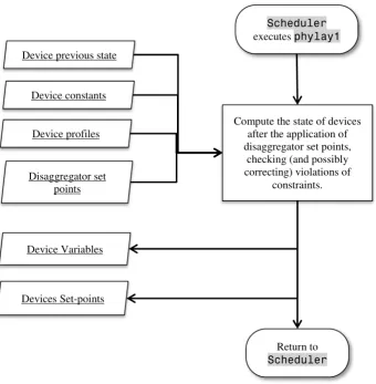
5.5.1 PHYLAY 1 ...108
5.5.2 PHYLAY 2 ...119
5.5.2.1 Simulation of DSO operations ...122
5.5.2.2 Simulation of TSO operations ...122
5.5.2.3 Updated states of devices ...127
5.6 Output to database ...134
6 Database tables...136
6.1 Devices ...136
6.1.1 Device Constants: ...136
6.1.2 Device Profiles ...136
6.1.3 TCL Aggregator internal tables ...139
6.1.4 Disaggregator set points ...140
6.1.5 Device and Network Variables ...140
6.1.6 Initial state of devices ...141
6.1.7 Final state of devices ...141
6.2 Network Model ...142
6.2.1 Network parameters ...142
6.2.2 Network Variables ...145
6.2.3 Final state of network ...145
6.3 Market tables ...147
6.3.1 Market Bids: ...147
6.3.2 Market Bid Constraints: ...149
6.3.3 Price profiles ...152
6.3.4 NodeNetInjection: ...152
6.3.5 Market Clearing: ...153
Copyright 2019 SmartNet Page 6
List of Abbreviations and Acronyms
Acronym Meaning
aFRR automatic Frequency Restoration Reserve
AL Atomic Load
AMPL A Mathematical Programming Language (software) CGCL Curtailable Generation Curtailable Load
CHP Combined Heat and Power
CON(V) Conventional Generator
CPLEX A mixed-integer linear programming solver offered by IBM (software)
CS Coordination scheme
DB Database
DSO Distribution System Operator EES Electrical Energy Storage
EV Electric Vehicle
mFRR manual Frequency Restoration Reserve OLTC On Load Tap Changer
OPF Optimal Power Flow
PF Power Flow
PHYLAY Physical Layer
PV Photovoltaic
SEL Sheddable Load
SQL Structured Query Language STATCOM Static Compensator
STO Storage
Copyright 2019 SmartNet Page 7
Executive Summary
The TSO-DSO coordination schemes proposed by SmartNet have been tested by means of dedicated simulations aimed at realistically reproducing the behavior of the electrical system and of the involved actors in hypothetical scenarios (expected 2030 situation of Italy, Denmark and Spain). The present report describes the software platform of the simulator which has been completely developed by the SmartNet team on the basis of the theoretical concepts in terms of aggregation/disaggregation, TSO-DSO interactions and responsibilities, market clearing strategies.
An exhaustive simulation of TSO-DSO coordination schemes requires the simulation of both transmission and distribution network, including all the power devices and source of flexibility which are connected to the electricity system. For this reason, all the software blocks managed by the simulation platform have been designed in order to manage large amount of data and the related algorithms have been designed by means of simplifications that define a trade-off between simplicity (low computational burden) and accuracy.
In order to test the main interactions among system actors, the simulator has been coded by defining three main layers:
• The market layer, which integrates the market clearing routines aimed at solving the forecasted
conditions of network imbalance and congestions by optimally activating the flexibility bids. It can have different structures depending on the implemented TSO-DSO coordination scheme (central market, central+local markets, etc.) and integrates the possibility of accepting complex bids submitted by distribution resources too.
• The bidding and dispatching layer, which implements the aggregation/disaggregation routines
that translate the flexibility of physical resources (both transmission and distribution ones) into profitable bids to be submitted to the market. It also convert the market directives into individual set-points to be sent to the activated resources.
• The physical layer, which simulates the physics behind each considered flexible power unit and the
Copyright 2019 SmartNet Page 8
These layers are composed by different blocks that can be called in sequence by a dedicated scheduler. Numerous settings can be set in order to simulate arbitrary market and bidding dynamics (market frequency, latency, time horizon).
Copyright 2019 SmartNet Page 9
1
The SmartNet Simulator
In order to allow distribution system resources to provide ancillary services to the power system, the project SmartNet proposed different TSO-DSO coordination schemes [1]. These interaction models, in addition to enable an efficient procurement and activation of reserves located ad distribution level, new ancillary services aimed at guaranteeing a better management of the distribution network (i.e. congestion management and balancing).
Each TSO-DSO coordination scheme has its own peculiarities and the performance is expected to be dependent on the application scenario. The objective of the project SmartNet consists of testing the proposed TSO-DSO interactions on the 2030 scenarios expected for Italy, Denmark and Spain. For this reason, a dedicated simulation platform has been realized in order to implement the main concepts developed within the project aimed at supporting the coordination between network operators. The structure of the simulator can be described as a sequence of three main blocks:
• The bidding and aggregation layer
It consists in the processes aimed at converting the flexibility of physical resources (located bot at transmission and distribution levels) into bids that guarantee a profit to their owner. In case numerous small resources are threated (such as the case of small distribution power units), these processes aggregates them in order to constructs completive flexibility bids.
Once the ancillary services market has selected the optimal activations, the accepted bids are processed by this layer in order to convert market directives into power set-points for the controlled physical resources (disaggregation).
This layer, described in detail in section 3, implements the algorithms proposed by [2].
• The market layer
It implements the market clearing algorithms aimed at optimizing the activations of the submitted bids for the simultaneous management of two ancillary services: balancing and congestion management. Depending on the TSO-DSO coordination scheme, these services are limited to the transmission network (the TSO is a buyer of flexibility) or extended to distribution network too (both TSO and DSO are buyer of flexibility).
In order to manage distribution resources and increase the competition, the implemented algorithms integrate the possibility of submitting bids with complex constraints, particularly useful for the management of (distribution) resources with rebound effects.
This layer, described in detail in section 4, implements the algorithms described in [3].
• The physical layer
It simulates the behavior of the physical devices connected to distribution and transmission grids on the basis of their internal states and set-points received by the bidding and dispatching layer. Their power exchanges are then computed in order to calculate the state of the electrical network.
Copyright 2019 SmartNet Page 10 of secondary frequency regulation and unwanted measures.
The functions implemented within this layer are described in section 5.
The following sub-sections describes the main concepts behind the developed simulation environment, illustrating how the time dimension, the sequence of the blocks are managed by the software environment and their interactions. In addition, from section 2 to section 6, each layer is described in detail by listing all the coded functions and database variables called during the simulation process.
1.1
Time axis of the simulation
The SmartNet simulation is structured in order to return, on a discrete-time axis, the situation of the network as well as the status of the flexible devices. These time steps, represented in Figure 1, correspond to the time instants in which relevant updates are experienced by the physical layer: they can be represented by the state variation of devices and/or network assets, as well as the instants in which information are communicated from/to the other simulation layers.
Figure 1 – Discrete-time axis for which the SmartNet simulator returns the network conditions
and status of devices. A time resolution of 15 minutes is hypothesized
According to the diagram proposed in Figure 1, the application of the set-points (returned by the bidding and dispatching layer) and the communication of the network/devices status (again to the bidding and dispatching layer) are simultaneous. However, since the application of the set-points of the devices (as well as the natural evolution of the non-controlled power units) produces effects on the network physical quantities that have to be kept monitored until the reception of new set-points. In fact, between two generic T-th and (T+1)-th steps, the power exchange of non-controlled devices can change, failures occurs, network operators take action (congestion management, aFRR), etc. For this reason, an additional time step (T+1)- is added in order to provide
Copyright 2019 SmartNet Page 11
• the set-points returned by the other layers are applied in T and, consequently, the device and network
status are updated;
• the updated status of the devices and of the network are communicated back to the other layer in the
same time instant;
• the application of the set-points and the evolution of non-flexible devices determine transients in the
network/devices status and their final values (steady state condition) are returned at (T+1)-.
• During the time elapsed from T to (T+1)-, the network/devices situation has evolved creating also new
imbalance and activating the aFRR.
Figure 2 – SmartNet simulator events reported on the discrete-time axis.
A time resolution of 15 minutes is hypothesized
The set-points communicated at time T to the physical layer and the successive network/device status evolution correspond to the result of a structured process that involves all the SmartNet simulation layers. A graphical representation of this process (corresponding to one time step iteration of the SmartNet simulator) is reported in Figure 3 and it shows the following main steps:
1. The past network/devices situation is collected for:
a. Physical layer – return a forecasting of the situation of the network/devices when the set-points will be applied (and beyond).
b. Bidding and dispatching layer – Calculating bids of resources that directly access to the market. c. Bidding and dispatching layer – Aggregating small units to access to the market.
2. The outputs of these three sub-processes are managed by the market layer in order to report them in the optimization functions of the market clearing algorithm. The market returns the optimal set-points of the modelled flexible resources aimed at solving energy balance and network congestions.
3. Once set-points have been disaggregated/managed by the bidding and dispatching layer, this last layer sends them to the physical one, as well as the set-points for the network asset controlled by the operators (e.g. tap changing transformers).
4. At this step, set-points are applied (T-th time step) and begin to produce effects on the devices and on network status.
Copyright 2019 SmartNet Page 12
a. resources subjected to forecasting error activate their assigned set-points only if their current flexibility margins allow them;
b. network operators perform corrective actions (curtailment of resources in case of congestions, aFRR activation in case of residual imbalance, etc.).
All these measures take time to be activated and, in order to evaluate their impact on the network state, their impact is reported at (T+1)- (immediately before the application of the new set-points,
simultaneously computed by the other layers).
6. Therefore, in correspondence of (T+1)- time step, the network is assumed to be:
a. Without congestions (solved by the market with mFRR activations and congestion management strategies performed by network operators)
b. Balanced (thanks to the activation of mFRR and aFRR)
c. Ready to receive new set-points by the other layers (in order to replace the activated reserves) 7. The process is repeated from step 1 for the computation of the set-points to be activated at T+1.
The diagram reported in Figure 3 already indicates some concepts related to the time dynamics of the system. The following sub-sections are explaining more in details the aspects of latency L and market clearing period Ts.
Copyright 2019 SmartNet Page 13
1.1.1
Aggregation/Market/Disaggregation Latency (from devices data collection to
application of set-points)
In real life, the execution of the bidding/market clearing/dispatching processes (also reported in Figure 3) isrequires computational burden and time. This means that, from the measured/estimated imbalance and congestion to the application of corrective set-points, there is a time latency. This latency may depend on several factors:
• size of the network;
• aggregation/disaggregation timing;
• amount of bids to be processed by market clearing algorithms;
• amount/complexity of constraints to be included in the optimization algorithms; • etc.
Taking into account the discrete-time axis defined at the beginning of the document, this latency L can be measured with the amount of time steps elapsed from the data collection (instant in which bidding/dispatching and market layers are querying the physical one) to the set-points application on resources. Figure 4 graphically reports the latency concept:
• when L=1 the network/devices are monitored till T-1, the set-points are communicated at T- and start to
produce effects on the physical layer starting from T;
• when L=2 the network/devices are monitored till T-2, the set-points are communicated at T- and start to
produce effects on the physical layer starting from T;
• when L=3 the network/devices are monitored till T-3, the set-points are communicated at T- and start to
produce effects on the physical layer starting from T.
In all the cases, after the application of the set-points, the physical layer autonomously evolves until the reception of new set-points at T+1. Therefore, as anticipated above, at (T+1)- the simulation results will report
Copyright 2019 SmartNet Page 14 Figure 4 – SmartNet simulation process: latency (the set-point calculation process consists
of a combination of aggregation, market and disaggregation routines)
1.1.2
Market clearing frequency
Previously, two important time quantities have been defined:
• the resolution (… T-1, T, T+1 …) of the discrete-time axis, on which the simulation results are reported; • the latency L of the set-points calculation, starting from the network/devices measurements.
In addition to these, another important parameter to be defined is represented by the market clearing frequency. In fact, it is not necessary to have a cleared market with the same time resolution adopted for the provision of the simulation results, but it can be arbitrarily selected on the basis of standard balancing/congestion management needs.
According to this, the frequency (period) TS is defined as the amount of time steps (referred to the simulation
Copyright 2019 SmartNet Page 15
• in order to provide the set-points at the generic time step T, aggregators and market can access only to
network/devices situations before (T-L) and only making forecast for the consecutive time steps (T > T-L);
• the market clearing frequency cannot be lower than 1;
• when TS>1, the intermediate network/devices situations have to be calculated by means of a dedicated
processes which are separated from the market one (modelling only the network/devices independent evolution and the possible interventions of network operators);
• in this last case, the market clearing and disaggregation processes return a series of set-points to be applied in the next time instants (not only at T, but also at T+1, T+2, … T+TS).
Figure 5 – SmartNet simulation process: market clearing frequency
1.1.3
Pipelining
The previous section reports scenarios in which the latency corresponds to the market clearing period (L = TS). However the possibilities are not limited to this situation.
In principle, the provision of set-points happens with a fixed timing (e.g. every 15 minutes a new series of set-points is provided to the devices/network). However, the process of generating these values can also be faster, with a latency L < TS (Figure 6). In this case the market clearing algorithms generally process the
Copyright 2019 SmartNet Page 16 Figure 6 – SmartNet simulation process: case for which L < TS
When L > TS the situation is more complex. Looking at Figure 7 it can be noticed that separate processes have
to be run in parallel in order to provide the required set-points at every TS. In this case, one of the processes
aimed at generating the set-points (layer (1)) has not visibility of the ones generated by the parallel processes (layer (2)) and vice versa. This aspect is, of course, a significant issue and this decoupling should be faced with appropriate techniques.
Copyright 2019 SmartNet Page 17
1.2
Simulation of the SmartNet TSO-DSO coordination schemes
The investigations performed by SmartNet have highlighted five different coordination schemes that describe the interactions between TSO and DSO for the management of flexible resources for the provision of ancillary services. These schemes are described in [1] and [3] and are represented by:
• A. Centralized ancillary services market model • B. Local ancillary services market model • C. Shared balancing responsibility model
• D. Common TSO-DSO ancillary services market model • E. Integrated flexibility market model
Having considered the concepts described within the previous section, a single iteration of the SmartNet simulator (detailed in Figure 3) is reported in the sequence diagram depicted in Figure 8. In this scheme (representing two hypothetical cases of L and TS) the processes responsible of generating and applying
set-points are highlighted with a red path, while the processes describing the network/devices independent evolution are highlighted with a green path.
Figure 8 – Path followed by a single iteration of SmartNet simulator for two different selections of L and TS
Copyright 2019 SmartNet Page 18
1.2.1
TSO-DSO coordination scheme A – Centralized ancillary services market model
In this scheme, the process describing the generation of individual set-points (one for each flexible resource) is reported in Figure 9. It can be noticed that, since the market includes only the transmission network model, the forecasted network status is required only at transmission level. According to [1], distribution grid
constraints can be potentially modelled within the central market clearing algorithm. This last case, however, would be extremely similar to coordination scheme D1 (in terms of simulation results) and, for this reason, this variant is not investigated. The sequence diagram showing the simulation steps of TSO-DSO coordination
scheme A is reported in Figure 9.
Copyright 2019 SmartNet Page 19
1.2.2
TSO-DSO coordination scheme B – Local ancillary services market model
In this coordination scheme, in addition to the centralized market, a local market is cleared at distribution level. The DSO has priority to procure the necessary flexibilities in the local market (i.e. for local congestion management and rebalancing of taken actions) and, after that, the remaining resources are forwarded to the
centralized market (which also includes transmission elements). The sequence diagram showing these steps is reported in Figure 10.
Copyright 2019 SmartNet Page 20
1.2.3
TSO-DSO coordination scheme C – Shared balancing responsibility model
This coordination scheme is fairly different with respect to the other ones, since the DSO is called to act with balancing responsibility and the management of transmission and distribution system is completely decoupled. The same basic sequence diagram can be considered representative of the two distinct processes (one
for distribution and one for transmission) and they are schematized in Figure 11.
Copyright 2019 SmartNet Page 21
1.2.4
TSO-DSO Coordination scheme D – Common TSO-DSO ancillary services market model
From the simulation perspective, this coordination scheme is identical to coordination scheme A, except for the integration of the distribution network model in the centralized market clearing. This means that, also the forecasting of the distribution network state has to be calculated and sent to the common market. The process of
generating individual set points is schematized in Figure 12.
Copyright 2019 SmartNet Page 22
1.2.5
Process describing the independent evolution of device status and
network
In real world, during the processing of aggregation/market/disaggregation routines, the controllable devices and the network states are subjected to independent evolution, which occurs because of the forecasting error that determines:
• deviations of resources from the set-points requested by the disaggregators; • unforeseen network congestions that requires re-dispatching of critical resources;
• residual network imbalance (consequence of the previous two points) that has to be managed
by means of aFRR activations.
The simulation environment takes into account the effects of the forecasting error on the application of set-points. The three considered points are processed by means of the sequence diagram reported in Figure 13, which describes how network/devices are evolving from the application of market/disaggregators set-points in T-1 to the time instant immediately before the application of the market/disaggregators set-points in T.
Figure 13 – Independent network evolution and operations during the bidding and market processes
Copyright 2019 SmartNet Page 23 Figure 14 – Application of individual set points for energy balancing and consequent network evolution
Copyright 2019 SmartNet Page 24
2
Scheduler
2.1
Brief description of the module
The SmartNet architecture has been designed in a way as to allow different companies to develop and run each their own blocks with as minimal necessary interactions as possible. For this reason, an architecture based on sequentially executable blocks has been chosen. This sequential execution order leads to a scheduler that just corresponds to a simple for loop over the blocks and just executes the
block.execute() method for each block. The scheduler defines the order in which blocks have to be executed. In particular, according to architecture described in section 1, three main blocks can be identified:
• Bidding and dispatching layer (described in section 3)
It simulates the processes that translate the status of the flexible units in bids to be transmitted to the market operator. These processes also include aggregation of small unit flexibilities in a single one (big enough to participate to the market). Secondly, once the market has returned a solution, this layer dispatches the set-points to the controllable units.
• Market layer (described in section 4)
It runs the optimization algorithms (market clearing routines) that return the optimal set-points that have to be applied in order to balance the considered electricity system. These set-points are communicated to the bidding and dispatching layer (some of them are aggregated) in order to be adequately dispatched to the resources of the physical layer.
• Physical layer (described in section 5)
It simulates the electrical behavior of the network and devices for a given set of set-points provided by the other layers (bidding and dispatching layer). This layer also includes the low-level controls of network operators on grid assets and devices for the management of network congestions and borders balancing (secondary frequency control).
2.2
The high level architecture
Copyright 2019 SmartNet Page 25 Figure 15 – Block sequence diagram: implementation in process, tables and directories
Copyright 2019 SmartNet Page 26
2.3
Input from database
This section lists and describes the tables where the data are read. It is important is to underline the control parameters that affect the behaviour of the module and that can be changed in order to simulate different scenario configurations.
• L_m: This is the Latency of the market. Latency is defined as the (integer) time (index)
difference by the time step at which the market calculates its outputs (atT) and the first tim step it calculates the outputs for (forT). This latency also implies that bidders should submit their bids by at least so much time in advance for the bids to be considered in the market.
• H_m: Length of the Horizon of the market. This is the [difference between the last and the first
forT that the market considers in its bids] + 1.
• rollingHorizonAggregatorAndMarket: When True, this indicates that the market is
run every time step. If False, the market will only be run every H_m time steps, so all decisions are final, since outputs for any single time step are only calculated once.
• disaggregateOnlyOncePerMarketClearing: If True, it disaggregators are called only
once for the entire time horizon. If False disaggregation is done every time step instead, in which case disaggregators have to produce only values for one iteration (at a time).
• disaggregateWithOnlyMostRecentPhylayToOutput: Determines which phylay
output is used to disaggregate. If False, disaggregators work with information from block
phylay2 (from older atT for forT where atT<forT-L_m already. If True, disaggregation happens only with phylay2 info produced at atT=forT–L_m.
2.4
List of functions of the module
run(scenarioId, overwrite_CS_code, marketSolver=’cplex’): This is the main scheduler function. One can specify the simulation to be carried out, the coordination scheme that has to be tested for this scenario and the solver that the market should use (cplex/gurobi). This function performs a loop that just calls the execute function of each block in a specific order. Different schedules are possible. For example it can be that the aggregator and market module are called for every loop iteration, or not. Some cases like these are described in the previous section where the meaning of the called parameters is described.
Copyright 2019 SmartNet Page 27
2.5
Output to database
Copyright 2019 SmartNet Page 28
3
Bidding and dispatching layer
The bidding and dispatching layer is responsible of translating the physical flexibility of power devices in bids (bidding section) to be processed by the market blocks. Once the market clearing algorithm has returned its results, the accepted activations are again processed by this layer (dispatching section) in order to convert them into individual set-points for the physical resources (managed by the physical layer).
Since the majority of the connected resources are located at distribution level and are characterized by small power flexibility, most of the time the bidding and dispatching processed are actually represented by aggregation and disaggregation functions, which merge together small resources in order to produce bids with larger quantities.
Copyright 2019 SmartNet Page 29
3.1
Atomic Loads Aggregation/Disaggregation module
3.1.1
Brief description of the module
This class performs the aggregation of atomic loads and produces the bids for the market block. An atomic load consists of a device for which the activation can be postponed for a while, but once started cannot be paused or interrupted. The flexibility is produced by checking what loads are available in the system, and anticipating or postponing some of them in a coordinated manner by solving a discrete optimization problem. In this simulation the AggregatorAL is used to provide demand response bids from wet appliances, ie. dishwashers, tumble-driers, washing machines. The system makes use of mixed-integer linear optimization and requires CPLEX.
The detailed description of the atomic loads aggregation/disaggregation model is found in [2]. What this model represents, in short, is the controlled postponed activation of wet appliance loads with a fixed power profile.
As with other aggregator modules, the atomic loads aggregator is created in the database by the
Scheduler and controlled by calling three functions:
• AggregatorAL.initialize
o Obtains scenario, nodes and networks data from the database, finds the bidding
node of each associated device node (the nodal resolution of the system varies with the simulated TSO-DSO coordination scheme). The flow diagram is represented in Figure 16.
• AggregatorAL.execute in mode “aggreg”
o In case of available devices for a specific network node, it creates a flexibility bid and
places it into the database. The flow diagram is represented in Figure 17.
• AggregatorAL.execute in mode “disagg”
o It activates the corresponding devices of a previously formulated bid that was
accepted by the market clearing module. The flow diagram is represented in Figure 18.
As with the other aggregator modules, the AggregatorAL is integrated to the Scheduler (see section 2) and retrieves any other necessary data from the database.
The database is initially populated with characteristics of each aggregated device (stored in
Copyright 2019 SmartNet Page 30 The database records associated with the AggregatorAL, as with other aggregators, are constantly modified by the physical layer. The physical layer will be updating these appliances through the use of
devices_WetVariables and the functions WetAggToVar and WetVarToDevOut. More information is available in section 5.
When the Scheduler calls the AggregatorAL.execute(“aggreg”), it updates its internal state of the time of activation of the available loads, possibly altered by the physical layer module.
As with other bidding modules, the results of the market clearing module also affects the
AggregatorAL. When calling the AggregatorAL.execute(“disagg”), the accepted bids involving this module are retrieved from the database. The module recovers the individual appliances involved in the bid formulation and activates them.
3.1.2
Input from other modules
The resources controlled by the AggregatorAL are inserted in the database by the scenario creation module.
The Scheduler can set up the aggressiveness of the AggregatorAL by adjusting the tail threshold. This represents unwanted rebound caused by the flexibility activation that will be carried beyond the current bidding window. If this value is too low, the algorithm is too conservative and no flexibility bids will be produced by the AggregatorAL. If it is too high, it means that possible large imbalances are being carried out of the simulation horizon. There is also the risk that the aggregator exhaust all its loads in the first moment and keeps none for future market iterations.
When calling AggregatorAL.execute the only arguments are related to the time window characteristics. There is atT, the time at which the aggregator is called and the latency L, which represents a future time step where the flexibility is actually needed. For instance, when called on aggregation mode, if atT=10 and L=3, the aggregator will look for loads that are still available at the time step 10 (they have not started yet) and will modify their activation in order to change the aggregated consumption profile as much as possible to the time slot forT=13.
Copyright 2019 SmartNet Page 31
3.1.3
Flow chart of the module
Figure 16 – Flow diagram of AggregatorAL.initialize
Scheduler initializes
AggregatorAL.initialize
devices_WetConstants
profiles_WetApplianceModel
profiles_WetApplianceProfile
profiles_WetApplianceBooting Distribution
Preprocessing and initialization
Initializes solver
Return to
Scheduler
Resources are aggregated for each
distribution node Actor
TSO-DSO coordination
scheme A? Resources are
aggregated for each transmission node
Solver available?
yes no
Raise exception
Copyright 2019 SmartNet Page 32
Figure 17 – Flow diagram of AggregatorAL.execute(“aggreg”)
Scheduler executes
AggregatorAL.execute(“aggreg”)
devices_WetConstants
Update available loads
Estimate flexibility cost for all prospected bids Gather all loads with the
same bidding node Collect flexibility bids, if any,
and imbalances (generate_flex_options)
Create exclusive QtBids at each bidding node
independently
Write to database
Any unprocessed bidding node?
Return to
Scheduler
bids_QtBid
bids_QBid
bids_QBidSegment
bids_ExclusiveChoiceConstraintOnQtBids_QtBid
yes
Copyright 2019 SmartNet Page 33
Figure 18 – Flow diagram of AggregatorAL.execute(“disagg”)
Scheduler executes
AggregatorAL.execute(“aggreg”)
Collect all accepted bids for each bidding node associated with the
AggregatorAL
For each one of them, collect the loads employed in the bid
construction
Return to
Scheduler
Update loads starting time according to the bid
requirements
disaggregators_setpoints_
WetAggOut clearing.models.
Copyright 2019 SmartNet Page 34
3.1.4
Output to database
The AggregatorAL.initialize adds only an instance of the Actor model representing the
AggregatorAL.
AggregatorAL.execute(“aggreg”) possibly creates a bid for the corresponding market iteration. Creating a bid requires the creation of linked records on the following database tables:
• QtBid, • QBid,
• QBidSegment.
If more than one single possible activation is returned by AggregatorAL.execute(“aggreg”), multiple records are added to QtBid, QBid and QBidSegment database tables. In this case, the instance of ExclusiveChoiceConstraintOnQtBids_QtBid is also created, in order to specify the mutually exclusive nature of the submitted flexibilities.
AggregatorAL.execute(“disagg”) stores the activations to be sent to physical devices on
Copyright 2019 SmartNet Page 35
3.2
TCL Aggregation module
3.2.1
Brief description of the module
The objective of the Thermostatically Controllable Loads (TCLs) Aggregation module is to combine the flexibilities provided by a portfolio of TCLs defining, as output, a set of flexibility bids to be delivered to a certain market session. The aggregation model assumes a direct load control scheme over the TCLs, where the control variable consists of the temperature set-point that can be deviated from the baseline temperature (in general, the comfort temperature set-point) between the upper and lower limits (previously agreed between the end-users and the Aggregator). End-users received an economic compensation in exchange for the loss of comfort. Based on this cost, the Aggregator defines the bidding price. The detailed model of TCLs aggregation is described in [2].
A preliminary step to the algorithm is to define all possible control strategies than can be applied to each TCL within the portfolio. For this purpose, a set of possible temperature set-points is defined by splitting the control (and end-user comfort) margins of each TCL into a set of equal-sized temperature levels. In addition, it is assumed that the durations of the control actions are variable varying from one time-step to a maximum duration equal to the market horizon. As a result, the total number of control actions that can be applied to each TCL is the multiplication of the total number of temperature levels by the total number of possible durations. Each possible control action will lead to obtain a different (mutually exclusive) flexibility bid.
The TCL Aggregator module implements two main steps, one for each control action:
1. Simulation of the individual flexibility profile of each TCL that is defined as the difference between the baseline power profile and the controlled one. For this purpose, a second-order thermal model describing the dynamics of the TCL is implemented. Discomfort costs are calculated based on the internal temperature deviation from the baseline temperatures.
2. Aggregation of the individual flexibility profiles and discomfort costs to build the aggregated flexibility bid to be delivered to the market.
Copyright 2019 SmartNet Page 36
3.2.2
Input from database
The inputs from the database required by the TCL Aggregation module are listed next: TCL Aggregator internal tables
• aggreg_AggregatorTcl
• aggreg_AvailabilityProfile
• aggreg_AvailabilityStep
• aggreg_BidConfig
• aggreg_ComfTempProfile
• aggreg_ComfTempStep
• aggreg_Device
• aggreg_Envelope
• aggreg_ExtTempProfile
• aggreg_ExtTempStep
• aggreg_ExtTGProfile
• aggreg_ExtTGStep
• aggreg_IntTGProfile
• aggreg_IntTGStep
• aggreg_MaxTempProfile
• aggreg_MaxTempStep
• aggreg_MinTempProfile
• aggreg_MinTempStep
• aggreg_Tcl
• aggreg_TclStatus
• aggreg_TimeStep
• tcls_FlexProfSet
• tcls_TempSetPointSet
Network parameters
• network_Node
• network_SubNetwork
• network_SubNetworkType
Copyright 2019 SmartNet Page 37 Price profiles
• profiles_NodeDeltaCost
• profiles_NodeDeltaCostProfile
• profiles_NodeHasNodeDeltaCostProfile
• profiles_NodePrice
• profiles_NodePriceProfile
• profiles_NodeHasNodePriceProfile
Scenario data
• scenario_Scenario
Devices set-points
• devices_setpoints_TclDevOut
3.2.3
Input from other modules
The only direct input of the TCL aggregation module is from the Scheduler, that provides at every market session the following parameters:
• Aggregation mode ("aggreg") • Scenario identifier
• Starting time-step of the simulation window • Market latency
• Market horizon
3.2.4
List of functions of the module
The TCL Aggregation module is based on an iterative process aimed at generating the flexibility bids. This process comprises a set of loops that iterate, for each TCL in the portfolio, all the possible control actions that can be applied to each TCL unit, i.e. temperature set-points set and control durations.
Copyright 2019 SmartNet Page 38
• Aggregator.py – Class AggregatorTCL
It implements the interface between the Scheduler and the TCL Aggregator/Disaggregator modules. Gets all the required data for the simulation (scenario, coordination scheme, simulation window, list of nodes, etc.) and calls the function that starts the aggregation process:
o AggregatorTCL.doAggregation starts the aggregation process.
o AggregatorTCL.updateStatusFromPhylay reads the latest status of TCL
units from the physical layer and updates the status within the aggregation model.
• node_aggregator.py – Class NodeAggregator
It contains the main processes for simulating the aggregation process, especially the logic for generating flexibility bids for all network nodes (that have TCL devices connected), and sends the generated bids to the market.
o NodeAggregator.doAggregation performs the practical aggregation. It
includes a loop for carrying out the aggregation process for each network node.
o NodeAggregator.sendBidsMarket saves the generated flexibility bids,
including bid constraints, into the database.
• tcl_aggregator.py – Class TCLAggregator
It contains the logic for simulating the aggregation process for all TCLs connected to a single network node. The main parameters of the simulation are initialised: list of available TCLs for control within the TCL set, the set of temperature set-points and the set of control durations to be simulated for each TCL connected to the specified node.
o TCLAggregator.doAggregation performs aggregation for all available TCLs, all
temperature set-points within the set-point set and all control durations within the control duration set.
• portfolio_flex.py – Class PortfolioFlexSimulator
It contains the logic for simulating the individual flexibility profiles for all TCLs in the TCL set.
o PortfolioFlexSimulator.simulateTcls: contains a loop for simulating each
TCL for all the possible temperature control set-points and control durations within the control duration set.
• set_point_flex.py – Class SetPointFlexSimulator
It contains the logic for simulating all temperature control set-points within the set-point set for a given TCL unit.
o SetPointFlexSimulator.simulateControlTemp: for a given TCL, contains a
Copyright 2019 SmartNet Page 39
• profile_flex.py – Class ProfilesFlexSimulator:
It contains the logic for simulating all control durations within the control duration set for a given TCL unit and temperature control set-point.
o ProfilesFlexSimulator.simulateProfiles: for a given TCL and
temperature control set-point, contains a loop for simulating each control duration within the control duration set.
• multi_step_flex.py – Class MultiStepFlexSimulator:
It contains the logic for simulating all time-steps within the simulation window for a given TCL unit, temperature control set-point and control duration.
o MultiStepFlexSimulator.simulatePeriod: for a given TCL, temperature
control set-point and control duration, contains a loop for simulating each time-step of the simulation window
• single_step_flex.py – Class SingleStepFlexSimulator
It contains the logic for simulating the behaviour of a TCL during a single time step.
o SingleStepFlexSimulator.simulateStep: implements the required
calculations to simulate individual flexibility and discomfort cost for a single time step when a particular temperature set-point and control duration is applied to a TCL unit. The calculation is based on a second-order thermal model. The evolution of the internal and envelope temperatures is also calculated as they are used as the initial values for the next time-step calculations.
3.2.5
Flow chart of the module
Copyright 2019 SmartNet Page 40
Copyright 2019 SmartNet Page 41
Copyright 2019 SmartNet Page 42
Figure 21 – Flow diagram of MultiStepFlexSimulator
3.2.6
Output to database
The TCL Aggregation module communicates with the other simulation blocks by writing in the database tables reported below:
TCL Aggregator internal tables
• aggreg_FlexCalculation
• aggreg_BidProfile
Copyright 2019 SmartNet Page 43 Bids
• bids_QBid
• bids_QBbidSegment
• bids_QtBid
Constraints
• constraints_ActivationDurationConstraint
• constraints_ExclusiveChoiceConstraintOnQtBids
Copyright 2019 SmartNet Page 44
3.3
TCL Disaggregation module
3.3.1
Brief description of the module
The objective of the TCL Disaggregation module is to translate the results of the market clearing process into control temperature set-points for the TCLs to attain the committed flexibility.
The implemented disaggregation process is straightforward since there is a direct link between the flexibility bids sent to the market and the individual control actions applied to the TCLs used to obtain them. So, when the market clearing results are known, the TCL Disaggregation module maps the accepted bids with the individual control set-points and sends them to the Physical Layer module.
3.3.2
Input from database
The inputs from the database required by the TCL Disaggregation module are listed next: Market clearing
• clearing_QBidSegmentVariables
• clearing_QBidVariables
• clearing_QtBidVariables
• clearing_SolveResult
Bids
• bids_QBid
• bids_QBidSegment
• bids_QtBbid
TCL Aggregator internal tables
• aggreg_FlexCalculation
• aggreg_BidProfile
• aggreg_BidCalculation
3.3.3
Input from other modules
Copyright 2019 SmartNet Page 45
• Aggregation mode ("disagg") • Scenario identifier
• Starting time-step of the simulation window
• Market latency • Market horizon
3.3.4
List of functions of the module
The main functions of the TCL Disaggregation module are described below. In a similar way as the TCL Aggregation module, it has been implemented following an object-oriented programming model in which each main function has been implemented in a different Class, and each Class in a different python module (*.py).
• Aggregator.py – Class AggregatorTCL
It implements the interface between the Scheduler and the TCL Aggregator/Disaggregator module.
o AggregatorTCL.doDisaggregation: starts the disaggregation process
• bid_disaggregator.py – Class BidDisaggregator
It contains the main entry point for simulating the disaggregation processes.
o BidDisaggregator.doDisaggregation: performs the disaggregation based
on the clearing results provided by the market module. As output, the temperature set-points of the TCLs for the Physical Layer module are generated.
3.3.5
Flow chart of the module
Copyright 2019 SmartNet Page 46
Figure 22 – Flow diagram of AggregatorTCL.execute(“disagg”)
3.3.6
Output to database
Outputs from the TCL Disaggregator module consist of individual control temperature set-points for each TCL that are written in the next table of the database:
Disaggregator set points
Copyright 2019 SmartNet Page 47
3.4
Conventional Generators Aggregation module
3.4.1
Brief description of the module
The objective of this module consists of defining flexibility bids for the conventional generators. A simplified model is implemented assuming that the flexibility of each generator corresponds to the difference between the maximum/minimum power and the baseline. According to this a bid is created for each time step (a single Qtbid composed by multiple Qbids) containing two segments: one for positive flexibility (baseline production to maximum capacity) and the other for negative flexibility (baseline production to technical minimum). Ramp constraints (RampConstraints) and reactive power capability (QPDiscConstraint) are also forwarded to the market module.
3.4.2
Input from database
The inputs from the database required by the Conventional Generators Aggregation module are listed next:
Device Constants:
• device_ConConstants
Device Profiles
• profiles_ConPowerProfile
• profiles_ConPower
Price profiles
• profiles_NodeDeltaCost
• profiles_NodeDeltaCostProfile
• profiles_NodeHasNodeDeltaCostProfile
• profiles_NodePrice
• profiles_NodePriceProfile
• profiles_NodeHasNodePriceProfile
Network parameters
• network_Node
Copyright 2019 SmartNet Page 48
• network_SubNetworkType
• network_Network
Device variables
• devices_ConVariables
Scenario data
• scenario_Scenario
3.4.3
Input from other modules
The only direct input is from the Scheduler that provides the following parameters each time the Conventional Generators Aggregation module is called::
• Aggregation mode ("aggreg") • Scenario identifier
• Starting time-step of the simulation window • Market horizon
• Market latency
3.4.4
List of functions of the module
The main functions of the Conventional Generators Aggregation module are described below:
• Aggregator.py – Class AggregatorCONV
It implements the interface between the Scheduler and the Conventional Generators Aggregation/Disaggregation module. It initializes all the required data for the simulation (scenario, coordination scheme, simulation window, list of nodes, etc.) and calculates the flexibility bids.
o AggregatorCONV.execute(“aggreg”): contains the main entry point for
simulating the aggregation process.
o AggregatorCONV.aggreg_bid: creates the flexibility bids of the conventional
generators
3.4.5
Flow chart of the module
Copyright 2019 SmartNet Page 49 the Scheduler, together with detailed data of the conventional generators including constants, variables and profiles. Network information is also required to know the generators connection nodes. The results consist of a set of flexibility bids per node that are stored in the bids and constraints tables.
Copyright 2019 SmartNet Page 50
3.4.6
Output to database
Outputs of the Conventional Generators Aggregation module are written in the following database tables:
Bids
• bids_QBid
• bids_QBidSegment
• bids_QtBid
Constraints
• constraints_QPDiscConstraint
Copyright 2019 SmartNet Page 51
3.5
Conventional Generators Disaggregation module
3.5.1
Brief description of the module
The objective of the Conventional Generators Disaggregation module is to translate the results of the market clearing process into power set-points for the conventional generators to attain the committed flexibility. The implemented disaggregation process is straightforward as each bid sent to the market is directly accepted or rejected.
3.5.2
Input from database
The inputs from the database required by the Conventional Generators Disaggregation module are listed as follows:
Market clearing
• clearing_QBidSegmentVariables
• clearing_QBbidVariables
• clearing_QtBidVariables
• clearing_SolveResult
Bids
• bids_QBid
• bids_QBidSegment
• bids_QtBid
3.5.3
Input from other modules
The disaggregation module takes as additional inputs the following parameters, which are provided by the Scheduler routine:
• Aggregation mode ("disagg") • Scenario identifier
• Starting time-step of the simulation window • Market latency
Copyright 2019 SmartNet Page 52
3.5.4
List of functions of the module
The main functions implemented in the Conventional Generators Disaggregation module are described below:
• Aggregator.py – Class AggregatorCONV
It implements the interface between the Scheduler and the Conventional Generators Aggregator/Disaggregation module.
o AggregatorCONV.execute(“disagg”)
It contains the main entry point for simulating the disaggregation process.
o AggregatorCONV.disaggreg_bid
It performs disaggregation based on the clearing results provided by the market module. As output, power set-points for the conventional generators for the physical layer module are generated.
3.5.5
Flow chart of the module
Copyright 2019 SmartNet Page 53
Figure 24 – Flow diagram of AggregatorCON.execute(“disagg”)
3.5.6
Output to database
Outputs from the Conventional Generators Disaggregation module consist of individual power set-points attributed to each conventional generator. These set-points are stored within the following database table:
Disaggregator set points
Copyright 2019 SmartNet Page 54
3.6
CHP Aggregation module
3.6.1
Brief description of the module
The objective of this module consists of generating flexibility bids for the Combined Heat and Power (CHP) units. A simplified algorithm is implemented: it assumes that the flexibility that can be provided by each unit corresponds to a portion (defined by a power availability factor) of the power bandwidth between the maximum/minimum power and the baseline. The availability factor represents a fraction of the maximum flexibility which limits the possible baseline deviations in order to do not significantly deviate from the nominal thermal demand.
According to this a bid is created for each time step (a single Qtbid composed by multiple Qbids) containing two segments: one for upward power flexibility and the other for downward negative flexibility. The reactive power capability (QPDiscConstraint) is also forwarded to the market module.
3.6.2
Input from database
The inputs from the database required by the CHP Aggregation module are listed next: Device Constants:
• device_ChpConstants
Profiles
• profiles_ChpPowerProfile
• profiles_ChpPower
• profiles_NodeDeltaCost
• profiles_NodeDeltaCostProfile
• profiles_NodeHasNodeDeltaCostProfile
• profiles_NodePrice
• profiles_NodePriceProfile
• profiles_NodeHasNodePriceProfile
Network parameters
• network_Node
• network_SubNetwork
• network_SubNetworkType
Copyright 2019 SmartNet Page 55 Device and Network Variables
• devices_ChpVariables
Scenario data
• scenario_Scenario
3.6.3
Input from other modules
The only direct input is from the Scheduler that provides the following parameters each time the CHP Aggregation module is called:
• Aggregation mode ("aggreg") • Scenario identifier
• Starting time-step of the simulation window • Market latency
• Market horizon
3.6.4
List of functions of the module
The main functions of the CHP Aggregation module are described below:
• Aggregator.py – Class AggregatorCHP
It implements the interface between the Scheduler and the CHP Aggregation/Disaggregation module. Initializes all the required data for the simulation (scenario, coordination scheme, simulation window, list of nodes, etc.) and calculates the flexibility bids.
o AggregatorCHP.execute(“aggreg”): contains the main entry point for
simulating the aggregation process.
o AggregatorCHP.aggreg_bid: creates the flexibility bids of the CHPs
3.6.5
Flow chart of the module
Copyright 2019 SmartNet Page 56
Copyright 2019 SmartNet Page 57
3.6.6
Output to database
Outputs of the CHP Aggregation module are stored within the following tables of the database: Bids
• bids_QBid
• bids_QBidSegment
• bids_QtBbid
Constraints