Multi-radio access network assignment using dynamic programming

Multi-Radio Access Network Assignment Using

Dynamic Programming

Vianney Anis and Stephan Weiss

Department of Electronic & Electrical Engineering, University of Strathclyde, Glasgow, Scotland {vianney.anis,stephan.weiss}@strath.ac.uk

Abstract—This paper addresses the formulation of an opti-misation problem that assigns a user to a multi-network base station for rural broadband access. The base station in this work is a fully off-grid—powered by renewable energy—system with a wireless backhaul link. The solution proposed in this paper relies on a dynamic programming approach, implementing a cost function that balances power consumption and quality of service. The cost is then aggregated using penalties based on the energy harvested and battery charge. The implemented algorithm is demonstrated (in simulations) able to adapt the user assignment to the network load and energy production.

I. INTRODUCTION

Information and communications technologies (ICTs) cur-rently represent approximately 10% of the world electricity consumption, and is forecast to reach 50% accounting for 23% of the humans carbon footprint by 2030 [1]. From those figures arises the question of the impact of ICTs on the environment. On the other hand, there is a substantial part of the world population with no or limited access to the internet; this is also true in remote area of economically developed countries such as the United Kingdom (UK) [2].

Typical broadband access solutions use an optical fibre network that is locally distributed to users through the copper twisted-pairs legacy phone network. However, the deployment of optical fibres is a very expensive process, which makes this technology unprofitable for service providers in low density areas. Adding to the network access issues, an unavailable or unreliable power grid at the base station site can represent further challenges and costs.

The suitability of wireless technologies for rural broadband has been studied in developing [3]–[6] and developed coun-tries [7]–[9], both from a technical and economical standpoint. Several wireless technologies were proposed in the context of rural broadband access, including Wireless Fidelity (WiFi) and TV white space (TVWS) approaches. The latter has been strongly motivated by the spectrum release that followed the Digital Television (DTV) switch-over in numerous countries such as the UK [10]. The remoteness of such base stations (BSs) might require the introduction of energy harvesters to supply power [11]–[13]. The introduction of renewable energy harvesting strongly affects the available power, two approaches are then possible to maintain service, either the energy system need to be overdimensioned to guarantee a minimum service [9] or resource management has to be introduced [14].

Previous studies [9] used wireless BSs to provide broadband

in remote areas, which have been successfully combined with various energy harvesters for power supply. Furthermore, the user spacial distribution in rural environments into the form of clusters—villages—surrounded by sporadically placed users renders the rural area well suited for the use of multiple radio access technologies with different propagation characteristics, allowing to serve both the close-by and farther away users to optimise the user data rate [15]. Several studies showed that energy savings are achievable by optimising the user assignment in a heterogeneous network scenarios [16], [17].

In this paper, using the BS design proposed in [9], we present a formulation of an optimisation problem of the user assignment on a base station concurrently employing two radio access technologies to provide broadband in rural area. The problem focussed on the minimisation of the power consumption of the BS under network capacity and harvested power constraints and is expressed to facilitate the use of a dynamic programming (DP) approach.

In Sec. II, we give details on the BS design, while Sec. III focuses on the power consumption and load model for the radio hardware and the energy production from the various re-newable energies harvesters. We then describe our formulation of the optimisation problem—based on a DP approach—in Sec. IV and finally provide results and analysis via simulation in Sec. V.

II. MULTI-RADIOOFF-GRIDBASESTATION

A. Radio Systems

WiFi

∼

6

km

∼

20

km

Fig. 1: Multi-radio access network scenario.

in the countryside are served by the TVWS network. This rural broadband access scenario—proved suitable in previous studies [3], [9], [15]—is presented in Fig. 1.

To optimise the assignment of users to either network, we as-sume that the users possess radio hardware that can be recon-figured for either the GHz or TVWS transmission channels. The user assignment to either of the TVWS or GHz network is managed by the BS. User radio hardware configurations as well as connection requests are transmitted using a low power, low data rate network covering the community in its entirety.

B. Power Supply and Storage

As in [9], the base station is powered by a single wind turbine (SuperWind SW350) with a peak output power of 350 W and two photovoltaic solar panels producing up to 250 W each. The use of multiple types of renewable energy sources provides the diversity to better safeguard a continuous power supply. In addition to the energy harvesters above, the base station uses a bank of Li-Ion batteries—12 V and 600Ah equivalent to a 7.2 kWh capacity—as an energy buffering and storage system.

III. SYSTEMMODEL

In this section, we present the various models we will be using in the cost and penalty function formulation.

A. Network Model

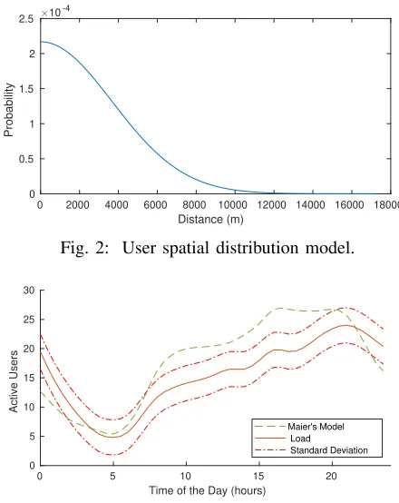
1) User Spatial Repartition: Rural environment is often composed of clusters of houses (i.e. a village) while other houses are spread sparsely around the community, sometime kilometres away from each other. In this study, we consider a village covering a circular area of 6 km in diameter, sur-rounded by single users located up to 14 km from the BS. To simplify the system model we place a single BS in the centre of the community and assume similar channel characteristic in all directions. Thus the users’ positions can then be simply expressed as their distance relative to the BS. Based on these assumptions, we used the half normal distribution shown in Fig. 2 to generate the position of N = 30 users in the community.

0 2000 4000 6000 8000 10000 12000 14000 16000 18000

Distance (m)

0 0.5 1 1.5 2

Probability

Fig. 2: User spatial distribution model.

0 5 10 15 20

Time of the Day (hours) 0

5 10 15 20 25 30

Active Users

Maier's Model Load Standard Deviation

Fig. 3: Mean load variation throughout the day.

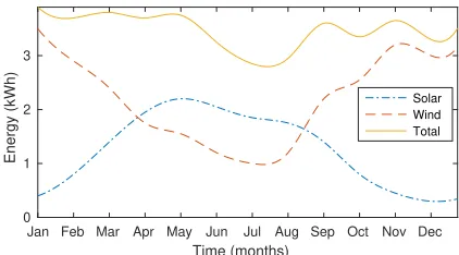
2) Load Model: As with every communication network the number of active users and thus the load on the base station varies, a typical approach would be to use a Maier model [20] to represent the evolution of the traffic over time. However, previously a study [9] of the ADSL traffic on the Isle of Tiree (UK) has shown that the load varied following the model presented in Fig. 3. The variation in the number of active users around the mean is modelled using a normal distribution with a standard deviation of 3 users. We assume however that at least one user is active at all times. This assumption while in theory not perfect represent a good approximation of a practical case in which we would need to keep at least the TVWS radio active to maintain service.

B. Power Consumption Model

In this paper, we used the power consumption model for the PTMP radio presented in [21]. The power consumption

Pa (in watts) of the radio systema∈ {g, u}, whereg andu

refer to the GHz and UHF radio access networks, respectively, can be expressed as follows:

Pa(t) =αa Patx(t)−G tx a

βa

+γa, (1)

where αa, βa, γa are coefficients characterising the radio a

power consumption model determined empirically by fitting to power consumption data from the BS in [9], [21]. The parameterGtx

a is the transmitting antenna gain and Patx(t)is

the minimum transmission power in dB required a the time stept,

P_atx(t) =La(d) +Parx−G rx

0 2000 4000 6000 8000 10000 12000 14000 Distance (m)

2.34 2.36 2.38 2.4 2.42 2.44

Power (W)

Fig. 4: GHz radio power consumption.

where Grx

a the receiving antenna gain, Parx the minimum

receiving power; d is the distance from the BS, d = rmax

for the TVWS network (a=u), where rmax is the distance to the farthest user and d = r(t) is the reach of the WiFi network at the time step t. The simplified pathlossLa(d)is

La(d) =Ka+η×10 log (d), (3)

as defined by [18]. Values of Ka and η, where determined

by pathloss measurement on the Isle of Tiree (UK) [21]. Using the parameters presented in Tab. I, we can then express the power consumption of the GHz radio as a function of the distance reached by the link, as shown in Fig. 4. Due to licensing issues the maximum transmit power for WiFi devices is limited to 30 dBm [22], thus restricting the maximum power consumption of the transmitting hardware.

To guaranty a full coverage of the community at all times the UHF network transmission power is set to reach the farthest user from the base station, we then have Ptx

u (t) =

Ptx

u (rmax). In addition to the PTMP radio consumption, the PTP backhaul link and the network equipment is estimated to consume approximately 45 W and 9 W, respectively [9].

C. Power Generation and Storage Models

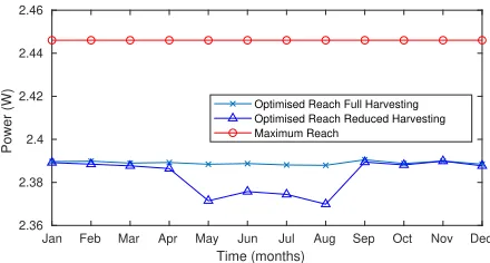
As with most renewable energy sources, the instantaneous power output of solar panels and wind turbines varies hourly, daily and monthly, thus we need a way to predict the available power at each time-step taking into account the time distri-bution of each energy source. Our work is based on data for energy harvested on the west coast of Scotland— Isle of Tiree and Bute—as presented in [9] The mean energy production of the two types of harvesters, listed in Sec. II-B, is presented in Fig. 5. These statistics show that the wind represents the main energy source during the winter months and that the increase

TABLE I: Power Consumption Model Parameters [15].

Parameter GHz UHF

η 2.39

αa 1.135e-7 3.395e-7

βa 4.545 4.424

γa 2.342 2.555

Ka −47.5dB −28.43dB

Prx

a −90dB −100dB

Grx

a 10dB 10dB

Jan Feb Mar Apr May Jun Jul Aug Sep Oct Nov Dec Time (months)

0 1 2 3

Energy (kWh)

Solar Wind Total

Fig. 5: Average daily energy generation on Tiree, Scotland [9].

in solar energy during the summer counterbalances the lack of wind power.

1) Solar Power: Photovoltaic electricity generation varies according to the weather, the time of the year and the hours of the day. In this work, the hourly energy distribution, as shown in Fig. 6, is estimated from the day length; for simplicity we suppose that the maximum energy can be harvested at midday. The instantaneous power output of a solar panel strongly depends on the amount of sunlight it receives, with its power output dropping down to 10% of its nominal output on a cloudy day. Using both hours of sunshine data [23] and hours of daylight per month, we compute the likelihood of a day to be sunny. This information is then used to randomly select the energy produced by the solar panels each day.

2) Wind Power: To keep the model simple we suppose that the wind is a slow varying resource at a day scale [24] while the solar energy varies greatly depending on the time of the day. However on a larger time-scale the wind is very unsteady and there can be a great difference in generation from one day to the next. Thus, we model the variation of energy in between days using a wide normal distribution withσw=µw/2. After

randomly selecting a value for each day, we model the slow hourly variation using interpolation between the produced data points.

3) Energy Storage: In this work we consider batteries with a capacity of 7.2 kWh and a charge/discharge efficiency of 80% [25]. This allows us to model the energy losses within the power management system as well as the natural self-discharge of the battery.

0 5 10 15 20

Time of the Day (hours) 0

20 40 60 80 100 120 140 160

Power (W)

January February March April May June July August September October November December

determine the boundary between the GHz and UHF networks based on energy optimisation. In the analysis in this section, terms such asEa,a={b, G, U, BS, . . .}, represent an energy

amount expressed in Joules (J), obtained from the correspond-ing power define in the models presented in Sec. III. For this study we discretised the time into 30 minutes time step δt,

indexed on the variablet.

A. Optimisation Problem

We aim to extract an optimum GHz radio reachropt(z=t)

for the current time steptout of the optimal breathing policy over a sliding window of 24 hours centred on the current time t for which we aim to find the best user assignment. This takes into account the current battery level and load, its values for the past 12 hours, and the forecasted energy generation and load for the next 12 hours. This relatively short window, indexed by z∈[t−24·δt;t+ 24·δt[, is motivated

by the limited reliability of forecasting [26]. We formulate the problem to determine the optimum policy r_opt over the 24-hour window

r_opt= arg min

r E(r) s.t. Eb(t)> Eb,min, (4)

NU≤NU,max,

where E(r) is an energy function related to the energy generation and consummation at the BS site over the each of the 24-hour window time steps, under quality of service constraints. The constraints for battery level Eb(t) left after we selected ropt(t) and the number of usersNU assigned to the TVWS limits the formed to a minimum valueEb,min, and the latter to the maximum number of supported usersNU,max, at any given time. The vector r= [Rt−24·δt, . . . Rt+24·δt]

T_,

over which the optimisation is to be performed, contains the range values of the GHz RAN, which for simplicity can take on the discrete distance values of theNusers, thus allowing us to index the possible values ofR usingn= 1, . . . , N. There are therefore 3049 _{different ways in which the GHz radio} access network can breath, and r_opt represents the optimum assignment over time.

The problem (4) can be addressed by a DP algorithm [27], which is divided into three steps. First we build a cost space based on the possible values for the reach of the GHz network and the BS load. Secondly, it aggregates the cost using a penalty function related to the harvested energy. Lastly, it generates a cost space were each cost related to a specific rtakes into account the past and future possible states of the network.

B. Cost Function

The cost function for thenth user at time stepz

C(z, n) =Cp(n) + µload·Cl(z, n), (5)

a control value µload. We express the power consumption as

Cp(n) =

EG(n) +EU+EBS+Ebackhaul

EGmax+EU+EBS+Ebackhaul

, (6)

i.e. as the ratio between the BS energy consumption associated with EG(n) and the maximum power consumption of the BS, linked to the maximum GHz radio energy consumption

EGmax. To balance the energy used by the GHz network to the energy requirements of the rest of the BS, we introduce the energy consumption of the TVWS radio hardware, EU, the energy consumption of the backhaul link radio,Ebackhaul, and the consumption of other subsystem in the BS,EBS.

While the cost Cp(n) increases with the coverage of the GHz network, theCl(z, n) decreases. We formulateCl(z, n) as

Cl(z, n) =  



Na(z)−n

Na(z)−N

whenNa(z)< N

Γload whenNa(z) =N

, (7)

whereNa(z)is the number of active number in the

commu-nity at timet. To prevent an infinite cost we introduceΓload when the number of active usersNa(z)is equal to the total

number of users N. The value of Γload is always set to be greater than any otherCl(z, n).

C. Cost Aggregation

Once the cost space C(z, n) is built, we proceed to the aggregation of the cost in both time directions. The aggregated cost towards negative time can be written as

L(−)(z, n) =C(z, n) + min

min

i≤n Pup(z) +L(−)(z−δt, i)

,

min

i≥n Pdown(z) +L(−)(z−δt, i)

(8)

with Pup and Pdown the penalties associated with an in-crease or dein-crease, respectively, of the GHz reach, such as

P{up,down}(z) =µ{up,down}(t)·G(z)whereG(z)is

G(z) = EW(z) +ES(z)

max t

EW(t) +ES(t)

, (9)

where EW(·) and ES(·) are the energy produced by the wind turbine and the solar panels, respectively. To keep the penalty values similar to the costC(z, n)we normaliseG(z)

using the maximum energy produced over the entire data. The parameterµ{up,down}(t), constant over the considered 24-hour window, allows for a finer control of the penalty as well as providing information on whether there is an increase or reduction in reach w.r.t. the previous time stept−δt:

µup(t) = max

Eb(t−δt)−Eb,min Cb

,0

(10)

0 10 20 30 40 50 Time of the Day (hours)

0 2000 4000 6000 8000 10000

Distance (m)

0 5 10 15 20 25 30

Active Users

WiFi Reach Position of Active User Number of Active User

Fig. 7: Two days simulation in January at full harvesting capacity.

with Cb the battery energy capacity expressed in Joules and Eb(t−δt) the energy available in the battery at the current

time step t on which the considered window is centred. The aggregated costs in each direction are then added together to produce an overall cost

L(z, n) =L(−)(z, n) +L(+)(z, n) ; (12)

where L(+)(z, n)represents the aggregation in positive time based on forecasted values. The quantity L(+)(z, n)is define analogously toL(−)(z, n)in (8) by replacingz−δtwithz+δt.

D. Optimum GHz Range Selection

The optimum reach breathing policy is selected by choosing for each z the value of n which minimises L(z, n), those values can be gathered into a vectornopt form which we can

get the optimal reach values ropt . The minimisation over

n is how restricted to users that are reachable by the GHz network. Furthermore, we have to ensure that the number of total active user NUassigned to the TVWS network is lower than the maximum number of users which the TVWS radio can serve under a quality of service constraint. By extracting the optimum reach policy we can determine the optimum reach for z=tand thus compute a related GHz radio energy consumption EG(t). We then calculate the energy left in the battery at the end of the time step t,Eb(t)such as

Eb(t) =αbEb(t−δt) +ηBS(EW(t) +ES(t))

− 1

ηBS

(EG(t) +EU+EBS+Ebackhaul)

(13)

the coefficient αb accounting for the battery self discharge and ηBS the efficiency of the power conversion systems. We are then ready to run the algorithm at the time step t+δt.

V. RESULTS

In order to test the performances of our algorithm, we ran simulation with a year worth of data randomly generated using the models described in Sec III, under two energy harvesting scenarios. The first considers the harvesting performances described in Secs. II-B and III while the second considers that the BS is equipped with harvesters providing only 25% of the energy output from the first scenario. The value of 25% was chosen empirically to maintain the battery level

0 5 10 15 20

Time of the Day (hours) 0

500 1000 1500 2000 2500 3000 3500

Distance (m) Jul: Full Harvesting Capacity

Jul: Reduced Harvesting Capacity Jan: Full Harvesting Capacity Jan: Reduced Harvesting Capacity

Fig. 8: Mean hourly GHz network reach on a day in January and July under full and reduced harvesting capacity.

above 10% over the all simulation. This reduced harvesting capacity simulation allows us to get a better understanding of the behaviours of the algorithm and considers the possibility to reduce the harvesting capacity of future BS designs. We used three metrics to judge the algorithm behaviour: the reach variation, the power consumption of the GHz radio as well as the number of users assigned to the TVWS network. We compute those metrics on a monthly basis and draw conclusions on the algorithm behaviours with regards to the mean harvested power presented in Fig. 5

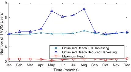
Fig. 7 shows the active users positions as well as the reach for the GHz network selected by the algorithm with respect to those positions over a two-day window. The number of active users confirms that the algorithm behaves as expected by adapting the GHz reach to the user activity, increasing the reach when numerous users are active and reducing it all the way to shutting down the GHz radio when all user can be served by the TVWS network. Fig. 8 presents the hourly average reach of the GHz network of the month of January and July, under the two considered scenario whereby January and July represent month with high and low harvested energy, respectively. The algorithm reduces the reach of the GHz radio in low energy condition, which is especially visible for the month of July under reduced harvesting capacity. This behaviour is corroborated by the reduction in power consumption for the GHz radio in Fig. 9, which is linked to the increase in the number of users assigned to the TVWS network as evident from Fig. 10.

Jan Feb Mar Apr May Jun Jul Aug Sep Oct Nov Dec

Time (months)

2.36 2.38 2.4 2.42 2.44 2.46

Power (W)

Optimised Reach Full Harvesting Optimised Reach Reduced Harvesting Maximum Reach

Jan Feb Mar Apr May Jun Jul Aug Sep Oct Nov Dec

Time (months)

5 6 7 8

Number of TVWS Users

Optimised Reach Full Harvesting Optimised Reach Reduced Harvesting Maximum Reach

Fig. 10: Average numbers of TVWS users

VI. CONCLUSIONS

In this paper, we have presented an energy model and optimisation process for the assignment of users in a single base station multi-radio network for rural broadband access. The algorithm uses a dynamic programming approach over a cost function defined as the linear combination of a power consumption and a network load related cost over a 24 hours sliding window.

The algorithm is effective in reducing the power consump-tion of the GHz PTMP radio, providing up to 3% energy saving against a maximum reach policy. Together with efforts towards a low-power basestation implementation [9], [28], [29], this algorithm can permit a downsizing of the power supply systems (harvesters and batteries), thus reducing the cost of the base station, as demonstrated in simulation by reducing the harvesting capacity of the BS to 25%. Further-more the algorithm can provide a better balance between the number of users assigned to each of the networks, and is therefore capable of enhancing the quality of service.

ACKNOWLEDGEMENT

This work has received funding by the European Union Horizon 2020 research and innovation programme under the Marie Skłodowska-Curie grant agreement No 675891 (SCAV-ENGE).

REFERENCES

[1] L. Hilty and B. Aebischer, eds., ICT Innovations for Sustainability. Advances in Intelligent Systems and Computing, Springer, 2015. [2] OfCom, “UK Home Broadband Performance: The performance of

fixed-line broadband delivered to UK residential consumers,”Research Report, p. 94, 2018.

[3] S. Roberts, P. Garnett, and R. Chandra, “Connecting africa using the TV white spaces: From research to real world deployments,” inThe 21st IEEE International Workshop on Local and Metropolitan Area Networks, pp. 1–6, Apr. 2015.

[4] A. Haider, R. Rahman, O. F. Noor, F. Alam, and R. M. Huq, “Towards an IEEE 802.22 (WRAN) based wireless broadband for rural Bangladesh — Antenna design and coverage planning,” in

2017 Int. Conf. Electrical, Computer and Communication Engineering, pp. 109–114, Feb. 2017.

[5] D. Espinoza and D. Reed, “Wireless technologies and policies for connecting rural areas in emerging countries: A case study in rural Peru,”Digital Policy, Regulation and Governance, Aug. 2018. [6] A. Singh, K. K. Naik, and C. R. S. Kumar, “UHF TVWS operation

in Indian scenario utilizing wireless regional area network for rural broadband access,” in 2016 Int. Conf. Next Generation Intelligent Systems, pp. 1–6, Sept. 2016.

2009.

[8] F. Darbari, M. Brew, S. Weiss, and W. S. Robert, “Practical aspects of broadband access for rural communities using a cost and power efficient multi-hop/relay network,” in2010 IEEE Globecom Workshops, pp. 731– 735, Dec. 2010.

[9] C. McGuire, M. R. Brew, F. Darbari, G. Bolton, A. McMahon, D. H. Crawford, S. Weiss, and R. W. Stewart, “HopScotch-a low-power renewable energy base station network for rural broadband access,”

EURASIP J. Wireless Comms & Networking, vol. 2012, no. 1, 2012.. [10] OfCom, “Digital dividend:cognitive access. Consultation on

licence-exempting cognitive devices using interleaved spectrum,” tech. rep., Feb. 2009.

[11] G. Schmitt, “The Green Base Station,” in4th International Telecom-munication - Energy Special Conference, pp. 1–6, May 2009. [12] J. Lorincz and I. Bule, “Renewable Energy Sources for Power Supply

of Base Station Sites,” Int. J. Business Data Communications and Networking, vol. 9, no. 3, pp. 53–74, 2013.

[13] K. Samdanis, P. Rost, A. Maeder, M. Meo, and C. Verikoukis,Green Communications: Principles, Concepts and Practice. John Wiley & Sons, 2015.

[14] F. Ahmed, M. Naeem, W. Ejaz, M. Iqbal, and A. Anpalagan, “Resource management in cellular base stations powered by renewable energy sources,”J. Network & Computer Appl., vol. 112, June 2018. [15] C. McGuire and S. Weiss, “Multi-radio network optimisation using

Bayesian belief propagation,” in2014 22nd European Signal Processing Conference, pp. 421–425, Sept. 2014.

[16] Y. Hou and D.I. Laurenson, “Energy Efficiency of High QoS Het-erogeneous Wireless Communication Network,” in 2010 IEEE 72nd Vehicular Technology Conference - Fall, pp. 1–5, Sept. 2010. [17] X. Zhang, Z. Su, Z. Yan, and W. Wang, “Energy-Efficiency Study for

Two-tier Heterogeneous Networks (HetNet) Under Coverage Perfor-mance Constraints,”Mob. Netw. Appl., vol. 18, pp. 567–577, Aug. 2013. [18] A. Goldsmith, Wireless Communications. New York, NY, USA:

Cambridge University Press, 2005.

[19] O. Holland, S. Ping, A. Aijaz, J. M. Chareau, P. Chawdhry, Y. Gao, Z. Qin, and H. Kokkinen, “To white space or not to White Space: That is the trial within the Ofcom TV White Spaces pilot,” in2015 IEEE International Symposium on Dynamic Spectrum Access Networks, pp. 11–22, Sept. 2015.

[20] G. Maier, A. Feldmann, V. Paxson, and M. Allman, “On Dominant Characteristics of Residential Broadband Internet Traffic,” inProc. 9th ACM SIGCOMM Conf. on Internet Measurement, New York, USA, pp. 90–102, 2009.

[21] C. McGuire and S. Weiss, “Power-optimised multi-radio network under varying throughput constraints for rural broadband access,” in 21st European Signal Processing Conference, pp. 1–5, Sept. 2013. [22] ETSI, “ETSI EN 300 328 V1.8.1 (2012-06) Electromagnetic

compat-ibility and Radio spectrum Matters (ERM); Wideband transmission systems; Data transmission equipment operating in the 2,4 GHz ISM band and using wide band modulation techniques; Harmonized EN covering the essential requirements of article 3.2 of the R&TTE Directive,” 2012.

[23] climatedata.eu, “Climate Glasgow - Scotland”, 2019. (https://www.climatedata.eu/climate.php?loc=ukxx0061&lang=en) [24] E. Hau and H. Von Renouard,The Wind Resource. Springer, 2006. [25] L. Gao, S. Liu, and R. A. Dougal, “Dynamic lithium-ion battery

model for system simulation,”IEEE Trans. Components and Packaging Technologies, vol. 25, pp. 495–505, Sept. 2002.

[26] J. Dowell, S. Weiss, D. Hill, and D. Infield, “Short-term spatio-temporal prediction of wind speed and direction,”Wind Energy, vol. 17, no. 12, pp. 1945–1955, 2014.

[27] M. Sniedovich,Dynamic Programming. New York, NY, USA: Marcel Dekker, Inc., 1991.

[28] V. Anis, C. Delaosa, L. H. Crockett, and S. Weiss, “Energy-efficient wideband transceiver with per-band equalisation and synchronisa-tion,” inIEEE Wireless Communications and Networking Conference, Apr. 2018.