Standard Steady State Genetic Algorithms Can Hillclimb Faster than Mutation-only Evolutionary Algorithms

White Rose Research Online URL for this paper:

http://eprints.whiterose.ac.uk/120316/

Version: Published Version

Article:

Corus, D. and Oliveto, P.S. (2017) Standard Steady State Genetic Algorithms Can

Hillclimb Faster than Mutation-only Evolutionary Algorithms. IEEE Transactions on

Evolutionary Computation. ISSN 1089-778X

https://doi.org/10.1109/TEVC.2017.2745715

[email protected] https://eprints.whiterose.ac.uk/ Reuse

This article is distributed under the terms of the Creative Commons Attribution (CC BY) licence. This licence allows you to distribute, remix, tweak, and build upon the work, even commercially, as long as you credit the authors for the original work. More information and the full terms of the licence here:

https://creativecommons.org/licenses/

Takedown

If you consider content in White Rose Research Online to be in breach of UK law, please notify us by

Standard Steady State Genetic Algorithms Can

Hillclimb Faster than Mutation-only Evolutionary

Algorithms

Dogan Corus,

Member, IEEE,

and Pietro S. Oliveto,

Senior Member, IEEE,

Abstract_{—Explaining to what extent the real power of genetic}

algorithms lies in the ability of crossover to recombine individuals into higher quality solutions is an important problem in evolu-tionary computation. In this paper we show how the interplay between mutation and crossover can make genetic algorithms hillclimb faster than their mutation-only counterparts. We devise a Markov Chain framework that allows to rigorously prove an upper bound on the runtime of standard steady state genetic algo-rithms to hillclimb theONEMAXfunction. The bound establishes that the steady-state genetic algorithms are 25%faster than all standard bit mutation-only evolutionary algorithms with static mutation rate up to lower order terms for moderate population sizes. The analysis also suggests that larger populations may be faster than populations of size 2. We present a lower bound for a greedy (2+1) GA that matches the upper bound for populations larger than 2, rigorously proving that 2 individuals cannot outperform larger population sizes under greedy selection and greedy crossover up to lower order terms. In complementary experiments the best population size is greater than 2 and the greedy genetic algorithms are faster than standard ones, further suggesting that the derived lower bound also holds for the standard steady state (2+1) GA.

I. INTRODUCTION

Genetic algorithms (GAs) rely on a population of individ-uals that simultaneously explore the search space. The main distinguishing features of GAs from other randomised search heuristics is their use of a population and crossover to generate new solutions. Rather than slightly modifying the current best solution as in more traditional heuristics, the idea behind GAs is that new solutions are generated by recombining individuals of the current population (i.e., crossover). Such individuals are selected to reproduce probabilistically according to their fitness (i.e., reproduction). Occasionally, random mutations may slightly modify the offspring produced by crossover. The original motivation behind these mutations is to avoid that some genetic material may be lost forever, thus allowing to avoid premature convergence [19], [17]. For these reasons the GA community traditionally regards crossover as the main search operator while mutation is considered a “background operator”[17], [1], [20] or a“secondary mechanism of genetic

adaptation” [19].

Explaining when and why GAs are effective has proved to be a non-trivial task. Schema theory and its resulting

D. Corus and P. S. Oliveto are with the Rigorous Research team, Algorithms group, Department of Computer Science, University of Sheffield, Regent Court, 211 Portobello, S1 4DP, Sheffield, UK. e-mail: {d.corus,p.oliveto}@sheffield.ac.uk., webpage: www.dcs.shef.ac.uk/people/P.Oliveto/rig/ .

building block hypothesis [19] were devised to explain such working principles. However, these theories did not allow to rigorously characterise the behaviour and performance of GAs. The hypothesis was disputed when a class of functions (i.e., Royal Road), thought to be ideal for GAs, was designed and experiments revealed that the simple (1+1) EA was more efficient [28], [21].

Runtime analysis approaches have provided rigorous proofs that crossover may indeed speed up the evolutionary process of GAs in ideal conditions (i.e., if sufficient diversity is available in the population). The JUMP function was introduced by Jansen and Wegener as a first example where crossover consid-erably improves the expected runtime compared to mutation-only Evolutionary Algorithms (EAs) [23]. The proof required an unrealistically small crossover probability to allow mutation alone to create the necessary population diversity for the crossover operator to then escape the local optimum. Danget al.recently showed that the sufficient diversity, and even faster upper bounds on the runtime for not too large jump gaps, can be achieved also for realistic crossover probabilities by using diversity mechanisms [6]. Further examples that show the effectiveness of crossover have been given for both artificially constructed functions and standard combinatorial optimisation problems (see the next section for an overview).

Excellent hillclimbing performance of crossover based GAs has been also proved. B. Doerr et al. proposed a (1+(λ,λ)) GA which optimises the ONEMAX function in

Θ(np

log log log(n)/log log(n))fitness evaluations (i.e., run-time) [8], [9]. Since the unbiased unary black box complexity of ONEMAX is Ω(nlogn) [25], the algorithm is asymptoti-cally faster than any unbiased mutation-only EA. Furthermore, the algorithm runs in linear time when the population size is self-adapted throughout the run [7]. Through this work, though, it is hard to derive conclusions on the working principles of standard GAs because these are very different compared to the (1+(λ,λ)) GA in several aspects. In particular, the (1+(λ,λ)) GA was especially designed to use crossover as a repair mechanism that follows the creation of new solutions via high mutation rates. This makes the algorithm work in a considerably different way compared to traditional GAs.

More traditional GAs have been analysed by Sudholt [40]. Concerning ONEMAX, he shows how (µ+λ) GAs are twice as fast as their standard bit mutation-only counter-parts. As a consequence, he showed an upper bound of

by any standard bit mutation-only EA [39], [42]. This bound further reduces to 1.19nlnn±O(nlog logn) if the optimal mutation rate is used (i.e., (1 +√5)/2·1/n ≈ 1.618/n). However, the analysis requires that diversity is artificially enforced in the population by breaking ties always preferring genotypically different individuals. This mechanism ensures that once diversity is created on a given fitness level, it will never be lost unless a better fitness level is reached, giving ample opportunities for crossover to exploit this diversity.

Recently, it has been shown that it is not necessary to enforce diversity for standard steady state GAs to outperform standard bit mutation-only EAs [5]. In particular, the JUMP

function was used as an example to show how the interplay between crossover and mutation may be sufficient for the emergence of the necessary diversity to escape from local optima more quickly. Essentially, a runtime of O(nk₋1_)may

be achieved for any sublinear jump length k > 2 versus the

Θ(nk_{)required by standard bit mutation-only EAs.}

In this paper, we show that this interplay between mutation and crossover may also speed-up the hillclimbing capabilities of steady state GAs without the need of enforcing diversity artificially. In particular, we consider a standard steady state (µ+1) GA [36], [17], [35] and prove an upper bound on the runtime to hillclimb the ONEMAXfunction of(3/4)enlogn+

O(n) for any µ ≥ 3 and µ = o(logn/log logn) when the standard 1/n mutation rate is used. Apart from show-ing that standard (µ+1) GAs are faster than their standard bit mutation-only counterparts up to population sizes µ =

o(logn/log logn), the framework provides two other inter-esting insights. Firstly, it delivers better runtime bounds for mutation rates that are higher than the standard 1/n rate. The best upper bound of 0.72enlogn+O(n)is achieved for

c/n with c = 1 2

√

13−1

≈1.3. Secondly, the framework provides a larger upper bound, up to lower order terms, for the (2+1) GA compared to that of any µ ≥ 3 and

µ = o(logn/log logn). The reason for the larger constant in the leading term of the runtime is that, for populations of size 2, there is always a constant probability that any selected individual takes over the population in the next generation. This is not the case for population sizes larger than 2.

To shed light on the exact runtime for population size

µ = 2 we present a lower bound analysis for a greedy genetic algorithm, which we call (2+1)S GA, that always selects individuals of highest fitness for crossover and always successfully recombines them if their Hamming distance is greater than 2. This algorithm is similar to the one analysed by Sudholt [40] to allow the derivation of a lower bound, with the exception that we do not enforce any diversity artificially and that our crossover operator is slightly less greedy (i.e., in [40] crossover always recombines correctly individuals also when the Hamming distance is exactly 2). Our analysis delivers a matching lower bound for all mutation rates c/n, where c is a constant, for the greedy (2+1)S GA (thus also

(3/4)enlogn+O(n)and0.72enlogn+O(n)respectively for mutation rates 1/n and1.3/n). This result rigorously proves that, under greedy selection and semi-greedy crossover, the (2+1) GA cannot outperform any (µ+1) GA with µ≥3 and

µ=o(logn/log logn).

We present some experimental investigations to shed light on the questions that emerge from the theoretical work. In the experiments we consider the commonly used parent selection that chooses uniformly at random from the population with replacement (i.e., our theoretical upper bounds hold for a larger variety of parent selection operators). We first compare the performance of the standard steady state GAs against the fastest standard bit mutation-only EA with fixed mutation rate (i.e., the (1+1) EA [39], [42]) and the GAs that have been proved to outperform it. The experiments show that the speedups over the (1+1) EA occur already for small problem sizesnand that population sizes larger than 2are faster than the standard (2+1) GA. Furthermore, the greedy(2 + 1)S GA indeed appears to be faster than the standard (2+1) GA1, further suggesting that the theoretical lower bound also holds for the latter algorithm. Finally, experiments confirm that larger mutation rates than1/nare more efficient. In particular, better runtimes are achieved for mutation rates that are even larger than the ones that minimise our theoretical upper bound (i.e.,c/nwith 1.5≤c≤1.6 versus thec=1.3 we have derived mathematically; interestingly this experimental rate is similar to the optimal mutation rate for OneMax of the algorithm analysed in [40]). These theoretical and experimental results seem to be in line with those recently presented for the same steady state GAs for the JUMP function [5], [6]: higher mutation rates than1/n are also more effective on JUMP.

The rest of the paper is structured as follows. In the next section we briefly review previous related works that consider algorithms using crossover operators. In Section III we give precise definitions of the steady state (µ+1) GA and of the ONEMAX function. In Section IV we present the Markov Chain framework that we will use for the analysis of steady state elitist GAs. In Section V we apply the framework to analyse the (µ+1) GA and present the upper bound on the runtime for any3≤µ=o(logn/log logn)and mutation rate

c/nfor any constantc. In Section VI we present the matching lower bound on the runtime of the greedy (2+1)S GA. In Section VII we present our experimental findings. In the Conclusion we present a discussion and open questions for future work. Separate supplementary files contain an appendix of omitted proofs due to space constraints and a complete version of the paper including all the proofs.

II. RELATEDWORK

The first rigorous groundbreaking proof that crossover can considerably improve the performance of EAs was given by Jansen and Wegener for the (µ+1) GA with an unrealistically low crossover probability [23]. A series of following works on the analysis of the JUMPfunction have made the algorithm characteristics increasingly realistic [6], [24]. Today it has been rigorously proved that the standard steady state (µ+1) GA with realistic parameter settings does not require artificial diversity enforcement to outperform its standard bit mutation-only counterpart to escape the plateau of local optima of the JUMP function [5].

Proofs that crossover may make a difference between poly-nomial and exponential time for escaping local optima have also been available for some time [37], [21]. The authors devised example functions where, if sufficient diversity was enforced by some mechanism, then crossover could efficiently combine different individuals into an optimal solution. Muta-tion, on the other hand required a long time because of the great Hamming distance between the local and global optima. The authors chose to call the artificially designed functions

Real Royal Roadfunctions because the Royal Road functions

devised to support the building block hypothesis had failed to do so [29]. The Real Royal Road functions, though, had no resemblance with the schemata structures required by the building block hypothesis.

The utility of crossover has also been proved for less artifi-cial problems such as coloring problems inspired by the Ising model from physics [38], computing input-output sequences in finite state machines [26], shortest path problems [14], vertex cover [30] and multi-objective optimization problems [33]. The above works show that crossover allows to escape from local optima that have large basins of attraction for the muta-tion operator. Hence, they establish the usefulness of crossover as an operator to enchance the exploration capabilities of the algorithm.

The interplay between crossover and mutation may produce a speed-up also in the exploitation phase, for instance when the algorithm is hillclimbing. Research in this direction has recently appeared. The design of the (1+(λ, λ)) GA was theoretically driven to beat the Ω(nlnn) lower bound of all unary unbiased black box algorithms. Since the dynamics of the algorithm differ considerably from those of standard GAs, it is difficult to achieve more general conclusions about the performance of GAs from the analysis of the (1+(λ, λ)) GA. From this point of view the work of Sudholt is more revealing when he shows that any standard (µ+λ) GA outperforms its standard bit mutation-only counterpart for hillclimbing the ONEMAXfunction [40]. The only caveat is that the selection stage enforces diversity artificially, similarly to how Jansen and Wegener had enforced diversity for the Real Royal Road function analysis. In this paper we rigorously prove that it is not necessary to enforce diversity artificially for standard-steady state GAs to outperform their standard bit mutation-only counterpart.

III. PRELIMINARIES

We will analyse the runtime (i.e., the expected number of fitness function evaluations before an optimal search point is found) of a steady state genetic algorithm with population size

µand offspring size 1 (Algorithm 1). In steady state GAs the entire population is not changed at once, but rather a part of it. In this paper we consider the most common option of creating one new solution per generation [36], [35]. Rather than restricting the algorithm to the most commonly used uniform selection of two parents, we allow more flexibility to the choice of which parent selection mechanism is used. This approach was also followed by Sudholt for the analysis of the (µ+1) GA with diversity [40]. In each generation the algorithm

Algorithm 1: (µ+1) GA [36], [17], [35], [5]

1 P ←µindividuals, uniformly at random from{0,1}n; 2 repeat

3 Selectx, y∈P with replacement using an operator

abiding (1);

4 z←Uniform crossover with probability1/2 (x, y); 5 Flip each bit inz with probabilityc/n;

6 P ←P∪ {z};

7 Choose one element from P with lowest fitness and

remove it fromP, breaking ties at random;

8 untiltermination condition satisfied;

picks two parents from its population with replacement using a selection operator that satisfies the following condition.

∀x, y: f(x)≥f(y) =⇒ Pr(select x)≥Pr(selecty). (1) The condition allows to use most of the popular parent selection mechanisms with replacement such as fitness pro-portional selection, rank selection or the one commonly used in steady state GAs, i.e., uniform selection [17]. Afterwards, uniform crossover between the selected parents (i.e., each bit of the offspring is chosen from each parent with probability

1/2) provides an offspring to which standard bit mutation (i.e., each bit is flipped with with probabilityc/n) is applied. The bestµamong theµ+ 1solutions are carried over to the next generation and ties are broken uniformly at random.

In the paper we use the standard convention for nam-ing steady state algorithms: the (µ+1) EA differs from the (µ+1) GA by only selecting one individual per generation for reproduction and applying standard bit mutation to it (i.e., no crossover). Otherwise the two algorithms are identical.

We will analyse Algorithm 1 for the well-studied ONEMAX

function that is defined on bitstringsx∈ {0,1}n _{of length n} and returns the number of1-bits in the string: ONEMAX(x) =

Pn

i=1xi. Here xi is the ith bit of the solution x ∈ {0,1}n. The ONEMAXbenchmark function is very useful to assess the hillclimbing capabilities of a search heuristic. It displays the characteristic function optimisation property that finding im-proving solutions becomes harder as the algorithm approaches the optimum. The problem is the same as that of identifying the hidden solution of the Mastermind game where we assume for simplicity that the target string is the one of all 1-bits. Any other target stringz∈ {0,1}n _{may also be used without loss} of generality. If a bitstring is used, then ONEMAXis equivalent to Mastermind with two colours [16]. This can be generalised to many colours if alphabets of greater size are used [12], [11].

IV. MARKOVCHAINFRAMEWORK

Fig. 1. Markov Chain for fitness leveli.

S1,i S2,i S3,i

1−pm−pd

pd

1−pc−pr

pr

pc

pm

number of diverse individuals on the local optima of the function. The analysis delivers improved asymptotic expected runtimes of the (µ+1) GA over mutation-only EAs only for population sizes µ=ω(1). This happens because, for larger population sizes, it takes more time to lose diversity once created, hence crossover has more time to exploit it. For ONEMAX the technique delivers worse asymptotic bounds for population sizes µ = ω(1) and an O(nlnn) bound for constant population size. Hence, the techniques of [5] cannot be directly applied to show a speed-up of the (µ+1) GA over mutation-only EAs and a careful analysis of the leading constant in the runtime is necessary. In this section we present the Markov chain framework that we will use to obtain the upper bounds on the runtime of the elitist steady state GAs. We will afterwards discuss how this approach builds upon and generalises Sudholt’s approach in [40].

The ONEMAX function has n+ 1 distinct fitness values.

We divide the search space into the following canonical fitness levels [22], [32]:

Li={x∈ {0,1}n|ONEMAX(x) =i}.

We say that a population is in fitness leveliif and only if its best solution is in level Li.

We use a Markov chain (MC) for each fitness level i to represent the different states the population may be in before reaching the next fitness level. The MC depicted in Fig. 1 distinguishes between states where the population has no diversity (i.e., all individuals have the same genotype), hence crossover is ineffective, and states where diversity is available to be exploited by the crossover operator. The MC has one absorbing state and two transient states. The first transient state

S1,iis adopted if the whole population consists of copies of the same individual at leveli(i.e., all the individuals have the same genotype). The second state S2,i is reached if the population consists of µ individuals in fitness level i and at least two individuals x and y are not identical. The second transient state S2,idiffers from the stateS1,iin having diversity which can be exploited by the crossover operator. S1,i andS2,i are mutually accessible from each other since the diversity can be introduced at stateS1,i via mutation with some probabilitypd and can be lost at state S2,iwith some relapse probability pr when copies of a solution take over the population.

The absorbing stateS3,iis reached when a solution at a bet-ter fitness level is found, an event that happens with probability

pmwhen the population is at stateS1,iand with probabilitypc when the population is at stateS2,i. We pessimistically assume that inS2,i there is always only one single individual with a

different genotype (i.e., with more than one distinct individual,

pc would be higher and pr would be zero). Formally when

S3,i is reached the population is no longer in level ibecause a better fitness level has been found. However, we will bound the expected time to reach the absorbing state for the next level only when the whole population has reached it (or a higher level). We do this because we assume that initially all the population is in level i when calculating the transition probabilities in the MC for each level i. This implies that bounding the expected times to reach the absorbing states of each fitness level is not sufficient to achieve an upper bound on the total expected runtime. When S3,i is reached for the first time, the population only has one individual at the next fitness level or in a higher one. Only when all the individuals have reached leveli+ 1(i.e., either in stateS1,i+1or S2,i+1)

may we use the MC to bound the runtime to overcome level

i+ 1. Then the MC can be applied, once per fitness level, to bound the total runtime until the optimum is reached.

The main distinguishing aspect between the analysis pre-sented herein and that of Sudholt [40] is that we take into account the possibility to transition back and forth (i.e., resp. with probability pd and pr) between states S1,i and S2,i as in standard steady state GAs (see Fig. 1). By enforcing that different genotypes on the same fitness level are kept in the population, the genetic algorithm considered in [40] has a good probability of exploiting this diversity to recombine the different individuals. In particular, once the diversity is created it will never be lost, giving many opportunities for crossover to take advantage of it. A crucial aspect is that the probability of increasing the number of ones via crossover is much higher than the probability of doing so via mutation once many 1-bits have been collected. Hence, by enforcing that once State

S2,i is reached it cannot be left until a higher fitness level is found, Sudholt could prove that the resulting algorithm is faster compared to only using standard bit mutation. In the standard steady state GA, instead, once the diversity is created it may subsequently be lost before crossover successfully recombines the diverse individuals. This behaviour is modelled in the MC by considering the relapse probability pr. Hence, the algorithm spends less time in stateS2,i compared to the GA with diversity enforcement. Nevertheless, it will still spend some optimisation time in stateS2,iwhere it will have a higher probability of improving its fitness by exploiting the diversity via crossover than when in stateS1,i(i.e., no diversity) where it has to rely on mutation only. For this reason the algorithm will not be as fast for ONEMAX as the GA with enforced diversity but will still be faster than standard bit mutation-only EAs.

An interesting consequence of the possibility of losing diversity, is that populations of size greater than 2 can be beneficial. In particular the diversity (i.e., State S2,i) may be completely lost in the next step when there is only one diverse individual left in the population. When this is the case, the relapse probability pr decreases with the population size

µ because the probability of selecting the diverse individual for removal is 1/µ. Furthermore, for population size µ = 2

for larger population sizes this is not the case. As a result our MC framework analysis will deliver a better upper bound for

µ > 2 compared to the bound for µ = 2. This interesting insight into the utility of larger populations could not be seen in the analysis of [40] because there, once the diversity is achieved, it cannot be lost.

We first concentrate on the expected absorbing time of the MC. Afterwards we will calculate the takeover time before we can transition from one MC to the next. Since it is not easy to derive the exact transition probabilities, a runtime analysis is considerably simplified by using bounds on these probabilities. The main result of this section is stated in the following theorem that shows that we can use lower bounds on the transition probabilities moving in the direction of the absorbing state (i.e., pm, pd and pc) and an upper bound on the probability of moving in the opposite direction to no diversity (i.e., pr) to derive an upper bound on the expected absorbing time of the Markov chain. In particular, we define a Markov chainM′ _{that uses the bounds on the exact transition}

probabilities and show that its expected absorbing time is greater than the absorbing time of the original chain. Hereafter, we drop the level indexifor brevity and useE[T1]andE[T2]

instead ofE[T1,i]andE[T2,i](Similarly,S1 will denote state

S1,i).

Theorem 1. Consider two Markov chains M and M′ _with the topology in Figure 1 where the transition probabilities for

M arepc,pm,pd ,prand the transition probabilities forM′

arep′

c,p′m,p′dandp′r. Let the expected absorbing time forM

beE[T]and the expected absorbing time ofM′ _{starting from} state S1 beE[T1′]respectively. If

•pm< pc •p′d≤pd •p′r≥pr

•p′c≤pc •p′m≤pm

Then E[T]≤E[T′

1]≤

p′_c+p′

r

p′_cp′_d+p′_cp′m+p′_mp′_r +

1

p′_c.

We first concentrate on the second inequality in the state-ment of the theorem which will follow immediately from the next lemma. It allows us to obtain the expected absorbing time of the MC if the exact values for the transition probabilities are known. In particular, the lemma establishes the expected times E[T1] andE[T2] to reach the absorbing state, starting

from the states S1 andS2 respectively.

Lemma 2. The expected times E[T1]and E[T2] to reach the absorbing state, starting from stateS1andS2respectively are as follows:

E[T1] = pc+pr+pd

pcpd+pcpm+pmpr ≤

pc+pr

pcpd+pcpm+pmpr

+ 1

pc

E[T2] =

pm+pr+pd

pcpd+pcpm+pmpr

.

Before we prove the first inequality in the statement of Theorem 1, we will derive some helper propositions. We first show that as long as the transition probability of reaching the absorbing state from the state S2 (with diversity) is greater

than that of reaching the absorbing state from the state with no diversity S1 (i.e., pm < pc), then the expected absorbing time from state S1 is at least as large as the expected time

unconditional of the starting point. This will allow us to achieve a correct upper bound on the runtime by just bounding the absorbing time from state S1. In particular, it allows us

to pessimistically assume that the algorithm starts each new fitness level in state S1 (i.e., there is no diversity in the

population).

Proposition 3. Consider a Markov chain with the topology given in Figure 1. Let E[T1] and E[T2] be the expected

absorbing times starting from state S1 and S2 respectively.

Ifpm< pc, thenE[T1]> E[T2] andE[T], the unconditional expected absorbing time, satisfiesE[T]≤E[T1].

In the following proposition we show that if we overes-timate the probability of losing diversity and underesoveres-timate the probability of increasing it, then we achieve an upper bound on the expected absorbing time as long as pm < pc. Afterwards, in Proposition 5 we show that an upper bound on the absorbing time is also achieved if the probabilitiespc and

pm are underestimated.

Proposition 4. Consider two Markov chainsM and M′ _with the topology in Figure 1 where the transition probabilities for M are pc,pm,pd, pr and the transition probabilities for

M′ _{are pc, pm, p}′

d and p′r. Let the expected absorbing times

starting from state S1 for M and M′ be E[T1] and E[T1′] respectively. Ifp′

d≤pd,p′r≥pr and pm< pc, thenE[T1]≤

E[T′

1].

Proposition 5. Consider two Markov chainsM and M′ _with the topology in Figure 1 where the transition probabilities for M are pc,pm,pd, pr and the transition probabilities for

M′ _{are p}′

c, p′m, pd and pr. Let the expected absorbing times

starting from state S1 for M and M′ be E[T1] and E[T1′] respectively. Ifp′

c≤pc andp′m≤pm, thenE[T1]≤E[T1′].

The propositions use that by lower boundingpd and upper boundingprwe overestimate the expected number of genera-tions the population is in stateS1compared to the time spent

in state S2. Hence, if pc > pm we can safely use a lower bound forpdand an upper bound forprand still obtain a valid upper bound on the runtime E[T1]. This is rigorously shown

by combining together the results of the previous propositions to prove the main result i.e., Theorem 1.

Proof of Theorem 1. Consider a third Markov chain M∗

whose transition probabilities are pc, pm, p′r, p′d. Let the absorbing time of M starting from state S1 be E[T1]. In

order to prove the above statement we will prove the following sequence of inequalities:

E[T]≤E[T1]≤E[T1∗]≤E[T1′].

According to Proposition 3,E[T]≤E[T1] sincepc > pm. According to Proposition 4 E[T1] ≤ E[T1∗] since p′d ≤ pd,

p′

r ≥ pr and pc > pm. Finally, according to Proposition 5,

p′

c ≤pc andp′m≤pmimplies E[T1∗]≤E[T1′] and our proof

is completed by using Lemma 2 to show that the last inequality of the statement holds.

current fitness level. Hence, by summing up the expected runtimes to leave each of the n+ 1 levels and the expected times for the whole population to takeover each level, we obtain an upper bound on the expected runtime. The next lemma establishes an upper bound on the expected time it takes to move from the absorbing state of the previous Markov chain (S3,i) to any transient state (S1,i+1orS2,i+1) of the next

Markov chain. The lemma uses standard takeover arguments originally introduced in the first analysis of the (µ+1) EA for ONEMAX [41]. To achieve a tight upper bound Witt had to carefully wait for only a fraction of the population to take over a level before the next level was discovered. In our case, the calculation of the transition probabilities of the MC is actually simplified if we wait for the whole population to take over each level. Hence in our analysis the takeover time calculations are more similar to the first analysis of the (µ+1) EA with and without diversity mechanisms to takeover the local optimum of TWOMAX[18].

Lemma 6. Let the best individual of the current population be in leveliand all individuals be in level at leasti−1. Then, the expected time for the whole population to be in level at least iis_O(µlogµ).

The lemma shows that, once a new fitness level is discov-ered for the first time, it takes at mostO(µlogµ)generations until the whole population consists of individuals from the newly discovered fitness level or higher. While the absorption time of the Markov chain might decrease with the population size, for too large population sizes, the upper bound on the expected total take over time will dominate the runtime. As a result the MC framework will deliver larger upper bounds on the runtime unless the expected time until the population takes over the fitness levels is asymptotically smaller than the expected absorption time of all MCs. For this reason, our results will require population sizes ofµ=o(logn/log logn), to allow all fitness levels to be taken over in expected

o(nlogn) time such that the latter time does not affect the leading constant of the total expected runtime.

V. UPPERBOUND

In this section we use the Markov Chain framework devised in Section IV to prove that the (µ+1) GA is faster than any standard bit mutation-only (µ+λ) EA.

In order to satisfy the requirements of Theorem 1, we first show in Lemma 7 that pc> pmif the population is at one of the finaln/(4c(1 +ec_{))fitness levels. The lemma also shows} that it is easy for the algorithm to reach such a fitness level. Afterwards we bound the transition probabilities of the MC in Lemma 8. We conclude the section by stating and proving the main result, essentially by applying Theorem 1 with the transition probabilities calculated in Lemma 8.

Lemma 7. For the (µ+1) GA with mutation ratec/nfor any constant c, if the population is in any fitness level i > n−

n/(4c(1+ec_{)), thenp}

cis always larger thanpm. The expected

time for the (µ+1) GA to sample a solution in fitness level

n−n/(4c(1 +ec_{))for the first time is O(nµlogµ).}

Proof. We consider the probability pc. If two individuals on the same fitness level with non-zero Hamming distance2dare selected as parents with probability p′_{, then the probability}

that the crossover operator yields an improved solution is at least (see proof of Theorem 4 in [40]):

Pr(X > d) =1

2(1−Pr(X =d)) =1

2

1−2−2d

2d d

≥1/4, (2)

where X is a binomial random variable with parameters 2d

and1/2 which represents the number of bit positions where the parents differ and which are set to1in the offspring. With probability(1−c/n)n _{no bits are flipped and the absorbing} state is reached. If any individual is selected twice as parent, then the improvement can only be achieved by mutation (i.e., with probability pm) since crossover is ineffective. So pc >

p′_{(1/4)(1−c/n)}n_{+ (1−p}′_{)pm, hence if pm< p}′_(1/4)(1−

c/n)n_+(1−p′_{)pmit follows thatpm< pc. The condition can}

be simplified topm<(1/4)(1−c/n)n with simple algebraic manipulation. For large enough n, (1−c/n)n _{≥1/(1 +e}c₎ and the condition reduces to pm<1/(4(1 +ec)).

Sincepm<(n−i)c/nis an upper bound on the transition probability (i.e., at least one of the zero bits has to flip to increase the ONEMAX value), the condition is satisfied for

i≥n−n/(4c(1 +ec_{)). For any leveli≤n−n/(4c(1 +e}c_)), after the take over of the level occurs inO(µlogµ)expected time, the probability of improving is at leastΩ(1)due to the linear number of 0-bits that can be flipped. Hence, we can upper bound the total number of generations necessary to reach fitness leveli=n−n/(4c(1 +ec_{))byO(nµlogµ).}

The lemma has shown that pc > pm holds after a linear number of fitness levels have been traversed. Now, we bound the transition probabilities of the Markov chain.

Lemma 8. Let µ ≥ 3. Then the transition probabilities pd,

pc,pr and pm are bounded as follows:

pd ≥

µ

(µ+ 1)

i(n−i)c2

n2_(ec_+O(1/n)), pc≥

µ−1 2µ2_(ec_+O(1/n)),

pr≤

(µ−1) 2µ−1 +O(1/n)

2ec_µ2_{(µ+ 1)} , pm≥

c(n−i)

n(ec_+O(1/n)).

Proof. We first bound the probabilitypdof transitioning from the state S1,i to the state S2,i. In order to introduce a new solution at leveliwith different genotype, it is sufficient that the mutation operator simultaneously flips one of the n−i

0-bits and one of the i 1-bits while not flipping any other bit. We point out that in S1,i, all individuals are identical, hence crossover is ineffective. Moreover, when the diverse solution is created, it should stay in the population, which occurs with probabilityµ/(µ+ 1)since one of theµcopies of the majority individual should be removed by selection instead of the offspring. So pd can be lower bounded as follows:

pd≥

µ

(µ+ 1)

ic n

(n−i)c n

Using the inequality (1−1/x)x₋1_{≥1/e≥(1−1/x)}x _{, we} now bound 1−nc

n−2

as follows:

1− c

n

n−2

≥1− c

n

n−1

≥1− c

n

n

=

1−_nc(n/c)−11−_nc

c

≥

1

e

1−_nc

c

≥_e1c

1−c 2

n

,

where in the last step we used the Bernoulli’s inequality. We can further absorb thec2_{/nin an asymptoticO(1/n)term as}

follows:

1−_nc

n₋2

≥e−c− O(1/n) = 1

ec_+O(1/n). (3) The bound for pd is then,

pd≥

µ

(µ+ 1)

i(n−i)c2

n2 _ec_+O(1/n).

We now consider pc. To transition from state S2,i to

S3,i (i.e., pc) it is sufficient that two genotypically different individuals are selected as parents (i.e., with probability at least 2(µ−1)/µ2_{), that crossover provides a better solution}

(i.e., with probability at least 1/4 according to Eq. (2)) and that mutation does not flip any bits (i.e., probability

(1 − c/n)n _{≥ 1/ e}c _+O(1/n)

according to Eq. (3)). Therefore, the probability is

pc≥2µ−1

µ2

1 4

1−_ncn ≥_2µ2_(ecµ₊−_O1_(1/n)) For calculatingprwe pessimistically assume that the Ham-ming distance between the individuals in the population is 2 and that there is always only one individual with a different genotype. A population in stateS2,i which has diversity, goes back to stateS1,i when:

1) A majority individual is selected twice as parent (i.e., probability(µ−1)2_/µ2_{), mutation does not flip any bit}

(i.e., probability(1−c/n)n_{) and the minority individual} is discarded (i.e., probability 1/(µ+ 1)).

2) Two different individuals are selected as parents, crossover chooses either from the majority individual in both bit locations where they differ (i,e., prob. 1/4) and mutation does not flip any bit (i.e., probability

(1−c/n)n _≤1/ec_{) or mutation must flip at least one} specific bit (i.e., probabilityO(1/n)). Finally, the minor-ity individual is discarded (i.e., probabilminor-ity1/(µ+ 1)). 3) A minority individual is chosen twice as parent and the

mutation operator flips at least two specific bit positions (i.e., with probabilityO(1/n2_{)) and finally the minority}

individual is discarded (i.e., probability1/(µ+ 1)). Hence, the probability of losing diversity is:

pr≤

1

µ+ 1

_(µ

−1)2

µ2

1−_ncn

+ 21

µ µ−1

µ

₁

4

1− c

n

n

+O(1/n)

+O(1/n2₎

≤ 2(µ−1)

2_{+ (µ−1) + 4e}c_{(µ−1)O(1/n)}

2ec_µ2_{(µ+ 1)} +

O(1/n2₎

µ+ 1 = (µ−1)[2(µ−1) + 1 + 4e

c_{O(1/n)] + 2e}c_µ2_O(1/n2₎

2ec_µ2_{(µ+ 1)}

= (µ−1)[2(µ−1) + 1 +O(1/n)] +O(1/n

2₎

2ec_µ2_{(µ+ 1)}

≤ (µ−1)(2_2ecµ_µ2−_(µ1 +_{+ 1)}O(1/n)).

In the last inequality we absorbed theO(1/n2_{)term into the} O(1/n)term.

The transition probability pm from state S1,i to state S3,i is the probability of improvement by mutation only, because crossover is ineffective at stateS1,i. The number of 1-bits in the offspring increases if the mutation operator flips one of the(n−i)0-bits ( i.e., with probability c(n−i)/n) and does not flip any other bit (i.e., with probability (1−c/n)n₋1 _≥

ec+O(1/n)−1 according to Eq. (3)). Therefore, the lower bound on the probabilitypmis:

pm≥

c(n−i)

n ec_+O(1/n).

We are finally ready to state our main result.

Theorem 9. The expected runtime of the (µ+1) GA withµ≥3

and mutation ratec/nfor any constant con ONEMAXis:

E[T]≤ 3e

c_nlogn

c(3 +c) +O(nµlogµ).

Forµ=o(logn/log logn), the bound reduces to:

E[T]≤ _{c(3 +}3 _c)ecnlogn(1 +o(1)).

Proof. We use Theorem 1 to bound E[Ti], the expected time until the (µ+1) GA creates an offspring at fitness leveli+ 1or above given that all individuals in its initial population are at level i. The bounds on the transition probabilities established in Lemma 8 will be set as the exact transition probabilities of another Markov chain,M′_{, with absorbing time larger than}

E[Ti](by Theorem 1). Since Theorem 1 requires thatpc> pm and Lemma 7 establishes that pc > pm holds for all fitness levels i > n−n/4c(1 +ec_{), we will only analyse E[T}

i] for

n−1 ≥i > n−n/ 4c(1 +ec₎

. Recall that, by Lemma 7, level n−n/ 4c(1 +ec₎

is reached in expectedO(nµlogµ)

time.

Consider the expected absorbing timeE[T′

i], of the Markov chain M′ _{with transition probabilities:}

p′d:=

µ

(µ+ 1)

i(n−i)c2

n2_(ec_+O(1/n)), p′c:=

µ−1 2µ2_(ec_+O(1/n)),

p′

r:=

(µ−1) 2µ−1 +O(1/n)

2ec_µ2_{(µ+ 1)} , p′m:=

c(n−i)

n(ec_+O(1/n)). According to Theorem 1:

E[Ti]≤E[Ti,′1]≤

p′

c+p′r

p′_cp′

d+p′cp′m+p′mp′r

+ 1

We simplify the numerator and the denominator of the first term separately. The numerator is

p′

c+p′r=

µ−1

2µ2_(ec_+O(1/n))+

(µ−1) 2µ−1 +O(1/n)

2ec_µ2_{(µ+ 1)}

≤ µ_2µ−2_e1c

1 + 2µ−1 +O(1/n)

µ+ 1

≤ (µ−₂1)[3_µ2_ecµ_(µ+_{+ 1)}O(1/n)]. (5)

We can also rearrange the denominator D =p′

cp′d+p′cp′m+

p′

mp′r as follows:

D=p′

c(p′d+p′m) +p′mp′r

=(µ−1)

_µi(n

−i)c2

(µ+1)n2(ec₊

O(1/n))+

c(n₋i)

n(ec₊ O(1/n))

2µ2_(ec_+O(1/n))

+c(n−i)(µ−1) 2µ−1 +O(1/n)

n(ec_{+O(1/n)) 2e}c_µ2_{(µ+ 1)} ≥

(µ−1)µi_(µ(n₊₁₎−i_n)c22 + c(n₋i)

n

2µ2_(e2c_+O(1/n))

+c(n−i)(µ−1) 2µ−1 +O(1/n)

n(e2c_{+O(1/n)) 2µ}2_{(µ+ 1)}

≥_2µc2(n_(e−2ci₊)(_Oµ−_(1/n1)₎₎·

_µic

(µ+ 1)n2 +

1

n+

2µ−1 +O(1/n)

n(µ+ 1)

≥_2µc2(n_(e−2ci₊)(_Oµ−_(1/n1)₎₎·

µic+ (µ+ 1)n+n 2µ−1 +O(1/n)

(µ+ 1)n2

!

≥

c(n−i)(µ−1)

µic+n

3µ+O(1/n)

2µ2_(e2c_{+O(1/n)) (µ+ 1)n}2 .

(6)

Note that the term in square brackets is the same in both the numerator (i.e., Eq. (5)) and the denominator (i.e., Eq. (6)) including the small order terms in O(1/n) (i.e., they are identical). LetA= [3µ+c′_{/n], wherec}′ _{>0 is the smallest}

constant that satisfies the O(1/n)in the upper bound on pr in Lemma 8. We can now put the numerator and denominator together and simplify the expression :

(p′

c+p′r)/ p′c(pd′ +p′m) +p′mp′r

≤ _2µ(2µ_e−c_(µ1)_{+ 1)}A ·

2µ2 _e2c_+O(1/n)

(µ+ 1)n2

c(n−i)(µ−1)(µic+nA)

≤ A e

2c_+O(1/n)

n2

ec_{c(n−i)(µic+nA)}.

By using that e2

c

+_O(1/n)

ec ≤ec+O(1/n), we get:

≤A(e

c₊

O(1/n))n2

c(n−i)(µic+nA)

≤ec An

2

c(n−i)(µic+nA)+O(1/n)

An2

c(n−i)(µic+nA).

The facts, n−i ≥ 1, A = Ω(1), and µ, i, c > 0 imply that, nA+µic= Ω(n) and _c(n−i)(An_µic2_+nA) = O(n). When multiplied by theO(1/n)term, we get:

≤ e

c_n

c(n−i)

An

(µic+nA)+O(1).

By adding and subtractingµicto the numerator of _(µicAn_+nA), we obtain:

≤ e

c_n

c(n−i)

1− µic

µic+nA

+O(1).

Note that the multiplier outside the brackets,(ec_n)/(c(n−

i)), is in the order ofO n/(n−i)

. We now add and subtract

µncto the numerator of−µicµic+nA to create a positive additive term in the order ofO µ(n−i)/n

.

= e

c_n

c(n−i)

1−_µicµnc_+nA+µ(n−i)c

µic+nA

+O(1) = e

c_n

c(n−i)

1− µnc

µic+nA

+ e

c_n

c(n−i)

µ(n−i)c µic+nA

+O(1) = e

c_n

c(n−i)

1−_µicµnc_+nA

+O(µ).

Sincep′

c = Ω(1/µ), we can similarly absorb 1/p′c into the

O(µ)term. After the addition of the remaining term1/p′

cfrom Eq.(4), we obtain a valid upper bound on E[Ti]:

E[Ti]≤

p′

c+p′r

p′

cp′d+p′cp′m+p′mp′r

+ 1

p′

c

≤ e

c_n

c(n−i)

1− µnc

µic+nA

+O(µ).

In order to bound the negative term, we will rearrange its denominator (i.e.,nA+µic):

n

3µ+c′_{/n] +µ= 3µn+c}′_+µic

= 3µn+c′−(n−i)µc+µnc < µn(3 +c) +c′,

where the second equality is obtained by adding and subtract-ingµnc. Altogether,

E[Ti]≤ e c_n

c(n−i)

1−_{µn(3 +}µnc_{c) +c′}

+O(µ) = e

c_n

c(n−i)

1−µnc+c ′ c

3+c −c′

c

3+c

µn(3 +c) +c′

+O(µ) = e

c_n

c(n−i)

1−_{3 +}c _c+ c

′ c

3+c

µn(3 +c) +c′

+O(µ) = e

c_n

c(n−i)

1− c

3 +c+O(1/n)

+O(µ) = e

c_n

c(n−i) 3

3 +c +O(µ).

on the runtime is: n

X

i=n₋n/(4c(1+ec₎₎

_ec_n

c(n−i) 3

3 +c +O(µ) +O(µlogµ)

≤

n

X

i=0

_ec_n

c(n−i) 3

3 +c +O(µlogµ)

≤3e

c_nlogn

c(3 +c) +O(nµlogµ)≤

3ec_nlogn

c(3 +c) (1 +o(1)),

where in the last inequality we useµ=o(logn/log logn)to prove the second statement of the theorem.

The second statement of the theorem provides an upper bound of (3/4)enlogn for the standard mutation rate 1/n

(i.e., c= 1) andµ=o(logn/log logn). The upper bound is minimised forc=1

2 √

13−1

. Hence, the best upper bound is delivered for a mutation rate of about 1.3/n. The resulting leading term of the upper bound is:

E[T]≤ 6e

1 2(

√

13−1)_nlogn

√

13−1 1 2

√

13−1

+ 3 ≈1.97nlogn.

We point out that Theorem 9 holds for any µ ≥ 3. Our framework provides a higher upper bound when µ = 2

compared to larger values of µ. The main difference lies in the probability pr as shown in the following lemma.

Lemma 10. The transition probabilities pm, pr, pc and pd

for the (2+1) GA, with mutation ratec/nandcconstant, are

bounded as follows:

pd≥

2 3

i(n−i)c2

n2_(ec_+O(1/n)), pc≥

1

8(ec_+O(1/n)),

pr≤

5

24ec +O(1/n), pm≥

c(n−i) (ec_+O(1/n))n. The upper bound onprfrom Lemma 8 is1/(8ec), which is smaller than the bound we have just found. This is due to the assumptions in the lemma that there can be only one genotype in the population at a given time which can take over the population in the next iteration. However, when µ= 2, either individual can take over the population in the next iteration. This larger upper bound on pr for µ = 2 leads to a larger upper bound on the runtime ofE[T]≤c+44

ec

nlogn

c (1 +o(1)) for the (2+1) GA. The calculations are omitted as they are the same as those of the proof of Theorem 9 where pr ≥

5/(24ec_{) +O(1/n)is used and µis set to 2.} VI. LOWER BOUND

In the previous section we provided a higher upper bound for the(2+1)GA compared to the(µ+1)GA with population size greater than 2 andµ=o(logn/log logn). To rigorously prove that the(2 + 1)GA is indeed slower, we require a lower bound on the runtime of the algorithm that is higher than the upper bound provided in the previous section for the (µ+ 1)

GA (µ≥3).

Since providing lower bounds on the runtime is a noto-riously hard task, we will follow a strategy previously used by Sudholt [40] and analyse a version of the (µ+1) GA with

Algorithm 2: (2 + 1)S GA

1 P ←µindividuals, uniformly at random from{0,1}n; 2 repeat

3 Choosex, y∈P uniformly at random amongP∗, the

individuals with the current best fitnessf∗_; 4 z←Uniform crossover with probability1/2 (x, y); 5 Flip each bit inz with probabilityc/n;

6 Iff(z) =f∗ and max

w_∈P∗(HD(w, z))>2 then

z←z∨arg max

w∈P∗

(HD(w, z));

7 P ←P∪ {z};

8 Choose one element from P with lowest fitness and

remove it fromP, breaking ties at random;

9 untiltermination condition satisfied;

greedy parent selection and greedy crossover (i.e., Algorithm 2) in the sense that:

1) Parents are selected uniformly at random only among the solutions from the highest fitness level (greedy selection).

2) If the offspring has the same fitness as its parents and its Hamming distance to any individual with equal fitness in the population is larger than 2, then the algorithm automatically performs an OR operation between the offspring and the individual with the largest Hamming distance and fitness, breaking ties arbitrarily, and adds the resulting offspring to the population i.e., we pes-simistically allow it to skip as many fitness levels as possible (semi-greedy crossover).

The greedy selection allows us to ignore the improvements that occur via crossover between solutions from different fitness levels. Thus, the crossover is only beneficial when there are at least two different genotypes in the population at the highest fitness level discovered so far. The difference with the algorithm analysed by Sudholt [40] is that the (2 + 1)S GA we consider does not use any diversity mechanism and it does not automatically crossover correctly when the Hamming distance between parents is exactly 2. As a result, there still is a non-zero probability of losing diversity before a successful crossover occurs. The crossover operator of the(2+1)S GA is less greedy than the one analysed in [40] (i.e., there crossover is automatically successful also when the Hamming distance between the parents is 2). We point out that the upper bounds on the runtime derived in the previous section also hold for the greedy(2 + 1)S GA.

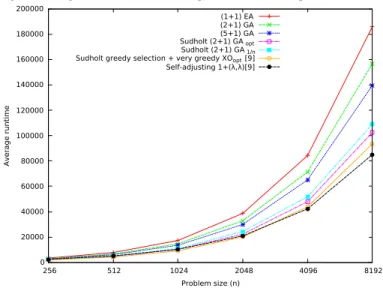
Fig. 2. Average runtime over 1000 independent runs versus problem sizen.

0 20000 40000 60000 80000 100000 120000 140000 160000 180000 200000

256 512 1024 2048 4096 8192

A

v

e

ra

g

e

r

u

n

ti

m

e

Problem size (n) (1+1) EA (2+1) GA (5+1) GA Sudholt (2+1) GAopt Sudholt (2+1) GA1/n Sudholt greedy selection + very greedy XO opt [9] Self-adjusting 1+(λ, λ)[9]

With population sizes greater than two, the loss of diversity can only occur when the majority genotype (i.e., the genotype with most copies in the population) is replicated. Building upon this we will show that the asymptotic performance of

(2 + 1)S GA for ONEMAX cannot be better than that of the (µ+1) GAs for µ >2.

Like in [40] for our analysis we will apply the fitness level method for lower bounds proposed by Sudholt [39]. Due to the greedy crossover and the greedy parent selection used in [40], the population could be represented by the trajectory of a single individual. If an offspring with lower fitness was added to the population, then the greedy parent selection never chose it. If instead, a solution with equally high fitness and different genotype was created, then the algorithm immediately reduced the population to a single individual that is the best possible outcome from crossing over the two genotypes. The main difference between the following analysis and that of [40] is that we want to take into account the possibility that the gained diversity may be lost before crossover exploits it. To this end, when individuals of equal fitness and Hamming distance 2 are created, crossover only exploits this successfully (i.e., goes to the next fitness level) with the conditional probability that crossover is successful before the diversity is lost. Otherwise, the diversity is lost. Only when individuals of Hamming distance larger than 2 are created, we allow crossover to immediately provide the best possible outcome as in [40].

Now, we can state the main result of this section.

Theorem 11. The expected runtime of the(2 + 1)S GA with

mutation probabilityp=c/nfor any constantconONEMAX

is no less than:

3ec

c

3 + max

1≤k≤n(

(np)k

(k!)2)

nlogn− O(nlog logn).

Note that forc≤4, max

1_≤k_≤n(

(np)k

(k!)2)≤pn=c. SinceE[T]≥

enlognforc≥3, for the purpose of finding the mutation rate that minimises the lower bound, we can reduce the statement

Fig. 3. Comparison between standard selection, greedy selection and greedy selection + greedy crossover GAs. The runtime is averaged over 1000 independent runs.

0 20000 40000 60000 80000 100000 120000 140000 160000

64 128 256 512 1024 2048 4096 8192

A

v

e

ra

g

e

r

u

n

ti

m

e

Problem size (n) (2+1) GA Greedy selection (2+1) GA (2+1)S GA Sudholt (2+1) GA1/n Sudholt greedy selection(2+1) GA1/n Sudholt greedy selection + greedy XO (2+1) GA1/n

of the theorem to:

3ec_nlogn

c(3 +c) − O(nlog logn).

The theorem provides a lower bound of (3/4)enlogn− O(nlog logn)for the standard mutation rate1/n(i.e., c = 1). The lower bound is minimised for c= 1

2 √

13−1

. Hence, the smallest lower bound is delivered for a mutation rate of about1.3/n. The resulting lower bound is:

E[T]≥ 6e

1 2(

√

13₋1₎

nlogn

√

13−1 1 2

√

13−1

+ 3− O(nlog logn) ≈1.97nlogn− O(nlog logn).

Since the lower bound for the (2 + 1)S GA matches the upper bound for the (µ+1) GA with µ > 2, the theorem proves that, under greedy selection and semi-greedy crossover, populations of size 2 cannot be faster than larger population sizes up to µ= o(logn/log logn). In the following section we give experimental evidence that the greedy algorithms are faster than the standard (2+1) GA, thus suggesting that the same conclusions hold also for the standard non-greedy algorithms.

VII. EXPERIMENTS

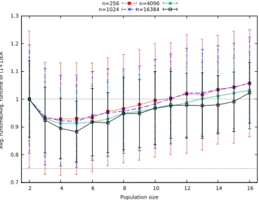
Fig. 4. Average runtime gain of the (µ+1) GA versus the (2+1) GA for different population sizes, errorbars show the standard deviation normalised by the average runtime forµ= 2.

0.7 0.8 0.9 1 1.1 1.2 1.3

2 4 6 8 10 12 14 16

A

v

g

.

ru

n

ti

m

e

/A

v

g

.

ru

n

ti

m

e

o

f

(1

+

1

)E

A

Population size n=256

n=1024

n=4096 n=16384

effects of the population size and mutation rate on the runtime of the steady-state GA for ONEMAXand compare its runtime against other GAs that have been proved to be faster than mutation-only EAs in the literature.

We start with an overview of the performance of the algorithms. In Fig. 2, we plot the average runtime over 1000 independent runs of the (µ+1) GA with µ = 2 and µ = 5

(with uniform parent selection and standard 1/n mutation rate) for exponentially increasing problem sizes and compare it against the fastest standard bit mutation-only EA with static mutation rate (i.e., the (1+1) EA with 1/n mutation rate). While the algorithm using µ = 5 outperforms the µ = 2

version, they are both faster than the (1+1) EA already for small problem sizes. We also compare the algorithms against the (2+1) GA investigated by Sudholt [40] where diversity is enforced by the environmental selection always preferring distinct individuals of equal fitness - the same GA variant that was first proposed and analysed in [23]. We run the algorithm both with standard mutation rate 1/n and with the optimal mutation rate (1 +√5)/(2n). Obviously, when diversity is enforced, the algorithms are faster. Finally, we also compare the algorithms against the (1+(λ,λ)) GA with self-adjusting population sizes and Sudholt’s (2+1) GA as they were compared previously in [10]. Note that in [10] (Fig. 8 therein) Sudholt’s algorithm was implemented with a very greedy parent selection operator that always prefers distinct individuals on the highest fitness level for reproduction.

In order to decompose the effects of the greedy parent selec-tion, greedy crossover and the use of diversity, we conducted further experiments shown in Figure 3. Here, we see that it is indeed the enforced diversity that creates the fundamental performance difference. Moreover, the results show that the greedy selection/greedy crossover GA is slightly faster than the greedy parent selection GA and that greedy parent selection is slightly faster than standard selection. Overall, the figure suggests that the lower bound presented in Theorem 11 is also valid for the standard (2+1) GA with uniform parent

selection (i.e., no greediness). In Figure 3, it can be noted that the performance difference between the GA with greedy crossover and greedy parent selection analysed in [40] and the (2+1) GA with enforced diversity and without greedy crossover is more pronounced than the performance difference between the standard (2+1) GA analysed in Section V and the

(2 + 1)S GA which was analysed in Section VI. The reason behind the difference in discrepancies is that the(2 + 1)S GA does not implement the greedy crossover operator when the Hamming distance is 2. We speculate that cases where the Hamming distance isjustenough for the crossover to exploit it occur much more frequently than the cases where a larger Hamming distance is present. As a result, the performance of the (2 + 1)S GA does not deviate much from the standard algorithm. Table I (see supplementary material) presents the mean and standard deviation of the runtimes of the algorithms depicted in Figure 2 and Figure 3 over 1000 independent runs. Now we investigate the effects of the population size on the (µ+1) GA. We perform 1000 independent runs of the (µ+1) GA with uniform parent selection and standard mutation rate 1/n for increasing population sizes up to µ = 16. In Fig. 4 we present average runtimes divided by the runtime of the (2 + 1)GA and in Fig. 5 normalised against the runtime of the (1+1) EA. In both figures, we see that the runtime improves for µ larger than 2 and after reaching its lowest value increases again with the population size. It is not clear whether there is a constant optimal static value forµaround 4 or 5. The experiments, however, do not rule out the possibility that the optimal static population size increases slowly with the problem size (i.e.,µ= 3forn= 256,µ= 4forn= 4096

andµ= 5forn= 16384). On the other hand, we clearly see that as the problem size increases we get a larger improvement on the runtime. This indicates that the harder is the problem, more useful are the populations. In particular, in Figure 5 we see that the theoretical asymptotic gain of 25% with respect to the runtime of the (1+1) EA is approached more and more closely as nincreases. For the considered problem sizes, the (µ+1) GA is faster than the (1+1) EA for all tested values of

µ. However, to see the runtime improvement of the (µ+1) GA against the (2+1) GA for µ > 15 the experiments (Fig. 4) suggest that greater problem sizes would need to be used.

Finally, we investigate the effect of the mutation rate on the runtime. Based on our previous experiments we set the population size to the best seen value ofµ= 5 and perform 1000 independent runs for each c value ranging from 0.9

to 1.9. In Figure 6, we see that even though the mutation rate c ≈ 1.3 minimises the upper bound we proved on the runtime, setting a larger mutation rate of1.6further decreases the runtime.

VIII. CONCLUSION

Fig. 5. Average runtime gain of the (µ+1) GA versus the (1+1) EA for different population sizes, errorbars show the standard deviation normalised by the average runtime of the (1+1) EA.

0.6 0.7 0.8 0.9 1 1.1 1.2 1.3 1.4

2 4 6 8 10 12 14 16

A

v

g

.

ru

n

ti

m

e

/A

v

g

.

ru

n

ti

m

e

o

f

(1

+

1

)E

A

Population size n=256

n=1024

n=4096 n=16384

Fig. 6. Average runtime gain of the (5+1) GA for various mutation rates versus the standard1/nmutation rate, errorbars show the standard deviation normalised by the average runtime for1/nmutation rate.

0.7 0.8 0.9 1 1.1 1.2 1.3

1 1.2 1.4 1.6 1.8

A

v

g

.

ru

n

ti

m

e

/

(

A

v

g

.

ru

n

ti

m

e

f

o

r

c

=

1

)

Mutation rate (c) n=256

n=1024

n=4096 n=16384

the (1+1) EA [21], [29]. In recent years it has been rigorously shown that crossover and mutation can outperform algorithms using only mutation. Firstly, a new theory-driven GA called (1+(λ,λ)) GA has been shown to be asymptotically faster for hillclimbing the ONEMAX function than any unbiased mutation-only EA [10]. Secondly, it has been shown how standard (µ+λ) GAs are twice as fast as their standard bit mutation-only counterparts for ONEMAX as long as diversity is enforced through environmental selection [40].

In this paper we have rigorously proven that standard steady-state GAs with µ≥3 andµ=o(logn/log logn) are at least 25% faster than all unbiased standard bit mutation-based EAs with static mutation rate for ONEMAX even if no diversity is enforced. The Markov Chain framework we used to achieve the upper bounds on the runtimes should be general

enough to allow future analyses of more complicated GAs, for instance with greater offspring population sizes or more sophisticated crossover operators. A limitation of the approach is that it applies to classes of problems that have plateaus of equal fitness. Hence, for functions where each genotype has a different fitness value our approach would not apply. An open question is whether the limitation is inherent to our framework or whether it is crossover that would not help steady-state EAs at all on such fitness landscapes.

Our results also explain that populations are useful not only in the exploration phase of the optimization, but also to improve exploitation during the hillclimbing phases. In particular, larger population sizes increase the probability of creating and maintaining diversity in the population. This diversity can then be exploited by the crossover operator. Recent results had already shown how the interplay between mutation and crossover may allow the emergence of diversity, which in turn allows to escape plateaus of local optima more efficiently compared to relying on mutation alone [5]. Our work sheds further light on the picture by showing that populations, crossover and mutation together, not only may escape optima more efficiently, but may be more effective also in the exploitation phase.

Another additional insight gained from the analysis is that the standard mutation rate 1/n may not be optimal for the (µ+1) GA on ONEMAX. This result is also in line with, and nicely complements, other recent findings concerning steady state GAs. For escaping plateaus of local optima it has been recently shown that increasing the mutation rate above the standard1/nrate leads to smaller upper bounds on escaping times [5]. However, when jumping large low-fitness valleys, mutation rates of about 2.6/n seem to be optimal static rates (see the experiment section in [3], [4]). For ONEMAX

lower mutation rates seem to be optimal static rates, but still considerably larger than the standard 1/n rate.

New interesting questions for further work have spawned. Concerning population sizes an open problem is to rigorously prove whether the optimal size grows with the problem size and at what rate. Also determining the optimal mutation rate remains an open problem. While our theoretical analysis deliv-ers the best upper bound on the runtime with a mutation rate of about 1.3/n, experiments suggest a larger optimal mutation rate. Interestingly, this experimental rate is very similar to the optimal mutation rate (i.e., approximately 1.618/n) of the (µ+1) GA with enforced diversity proven in [40]. The benefits of higher than standard mutation rates in elitist algorithms is a topic that is gaining increasing interest [31], [2], [15].