This is a repository copy of
Size Limited Iterative Method: A Hybridized Heuristic for Train
Unit Scheduling Optimization
.
White Rose Research Online URL for this paper:
http://eprints.whiterose.ac.uk/150722/
Version: Accepted Version
Proceedings Paper:
Copado-Mendez, P, Lin, Z and Kwan, R (2018) Size Limited Iterative Method: A Hybridized
Heuristic for Train Unit Scheduling Optimization. In: 14th International Conference on
Advanced Systems in Public Transport (CASPT). 14th International Conference on
Advanced Systems in Public Transport (CASPT), 23-25 Jul 2018, Brisbane, Australia. .
[email protected] https://eprints.whiterose.ac.uk/
Reuse
Items deposited in White Rose Research Online are protected by copyright, with all rights reserved unless indicated otherwise. They may be downloaded and/or printed for private study, or other acts as permitted by national copyright laws. The publisher or other rights holders may allow further reproduction and re-use of the full text version. This is indicated by the licence information on the White Rose Research Online record for the item.
Takedown
If you consider content in White Rose Research Online to be in breach of UK law, please notify us by
CASPT 2018
Size Limited Iterative Method: A Hybridized Heuristic
for Train Unit Scheduling Optimization
Pedro J. Copado-Mendez · Zhiyuan Lin · Raymond S. K. Kwan
Received: date / Accepted: date
Abstract In this research is presented an hybrid approach based on heuris-tics for solving large instances for the Train Unit Scheduling Optimization (TUSO). TUSO has been modelled as an Integer Multi-Commodity Flow Prob-lem (IMCF) lay on a Directed Acyclic Graph (DAG), and solved by Integer Linear Programming (ILP). This method proceeds in a way to iteratively im-prove the quality of one or more given feasible solutions by solving reduced instances of the original problem where only a subset of the arcs in the DAG are heuristically chosen to be optimised. Our approach is designed for reducing the original DAG into a much smaller size, but still retaining all the essential arcs for the optimal solution as much as possible. The capabilities of this frame-work for train unit scheduling optimization are tested by real-world cases and compared with the results from running the ILP solver alone for the original full problem instance and with the manual solutions for each dataset.
Keywords Train Unit Scheduling Optimization · Hybrid approach ·
Heuristics
1 Introduction
A train unit is a reversible non-splittable fixed set of train cars, which can be coupled/decoupled with other units of the same or compatible types if it is
P.J. Copado-Mendez, Raymond S.K. Kwan School of Computing, University of Leeds Leeds LS2 9JT
Tel.: 0113 343 5430
E-mail: p.j.copado-mendez, [email protected]
Zhiyuan Lin
Alliance Manchester Business School The University of Manchester Manchester M13 9SS
required. The train unit is the most commonly used passenger rolling stock in UK, Europe and many other countries, because of its well-known advantages over locomotives/wagons such as energy efficiency, acceleration and shorter turnaround times. Nonetheless, it still has to face the high costs associated with leasing, operating and maintaining a fleet. Hence, given a rail operators timetable on one operational day, a fleet of train units of different types and a rail network of routes, stations and infrastructures, Train Unit Scheduling Optimization (TUSO) (Lin, 2014) aims at determining the appropriately as-signment plan such as each trip is covered by a single or coupled units in order to satisfice the passenger demand. Note that TUSO is NP-hard problem as is proved in Schrijver (1993); Chen (2005); Cacchiani et al (2010); Lin and Kwan (2017).
For dealing with TUSO is formulated as Integer Multi-Commodity Flow (IMCF) problem based on Directed Acyclic Graph (DAG) (Ahuja et al, 1993; Cacchiani et al, 2010) and they solved by Linear Programming (LP) based heuristic Cacchiani et al (2013) or exact methods Cacchiani et al (2010); Lin and Kwan (2016). The particular problem scenario of TUSO in the UK is studied in Lin and Kwan (2013, 2014). A two-phase approach has been devel-oped, where in the first phase the assignment of train units to trips is carried out without considering station layout details Lin and Kwan (2014), whilst in the second phase the fleet assignment is implemented in terms of shunting movements, unit order and blockage of units, where the station infrastructure is taken into account Lei et al (2017). In addition, in Lin and Kwan (2016), a branch-and-price ILP model has been designed to solve the first phase exactly for medium sized instances, but it is difficult to handle large sized instances due to its exact nature. In order to deal with this limitation, in Copado-Mendez et al (2017) a hybrid approach combining the exact solver and a heuristic framework was introduced and treated in this work.
very close to an optimal solution. The hybrid framework design is challenging since there is a huge number of possible combination subsets of arcs that can form a feasible solution, and how the hybrid framework will pick up these op-timal ones from a rough initial feasible solution through a series of iterations is non-trivial.
The remainder of this paper is organized as follows. In Section ??, the literature review. Problem description in Section 2. Moreover, the SLIM ap-proach is described in Section 3. Finally, an extensive experimental evaluation is provided in Section 4 and conclusions as well as an outlook to future work is given in Section 6.
2 Problem Description
The problem aims at covering all timetabled trips for an operational day us-ing the minimum number of train units and reducus-ing the operational cost. Two or more units can be coupled together to meet the high passenger de-mand of a train trip. Different types of train units may be incompatible to be coupled, and coupling/decoupling operations may not be allowed at some locations. This problem is transformed into a network framework based on DAG denoted byG = (N,A), where the node setN =NS{s, s′} is the set
of train services, and s and s′ are the source and sink node. The arc set is
defined as A=ASA0, whereA={(i, j)|i, j∈ N }is the connection-arcset
andA0={(s, j)|j∈ N } ∪ {(j, s′)|j∈ N }is thesign-on/offarc set.
Each arc (i, j) stands for the potential linkage relation between tripiand trip j to be served by the same unit at the same station (same-location arc) or different stations (empty-running arc) also called empty-running (ECS). Given trip i has origin and destination denoted by io
and id
and departure and arrival time that are represented asid
t andi o
t respectively.
Finally, an s−s′ path in G represents a sequenced daily workload (the
train nodes in the path) for a possible unit schedule or diagram and the flow on it indicates the number of units used for serving those trains. Details of this DAG representation can be found in Lin and Kwan (2016).
3 Description of SLIM
will be henceforth denoted by Rolling Stock Optimization (RS-Opt). Hence, the method presented here is an attempt to overcome the RS-Opt limitations, solving reduced instances of the original problem by means of the RS-Opt which is iteratively called as a black-box.
Our approach, Size Limited Iterative Method (SLIM), is based on the gen-eral idea that a optimal solution (or whatever solution) is a sub-graph com-posed of all nodes of the original graph but only a small fraction of arcs, i.e. theessentialarcs connecting the source and sink nodes through paths covering all nodes. We henceforth refer to this sub-graph asEssential Arcs Graph de-noted byG. By adding a small quantity of new arcs fromGto thisG, it can be extended toAugmented Arcs Graph denoted byGb. A newG′ is obtained after solving this augmented arcs graph, which is better or equal than the previous
b
G. If these operations (G →G →b RS-Opt →Gb′) are repeated sequentially
several iterations then it is expected reach high-quality (sub-)optimal solution in a reasonable time.
SLIM strives to seek the optimal G∗ over all possibleGb’s, starting from a given initialG0. The size ofGbis limited by real value 0< µ <1. Thisµis
care-fully calibrated in order to solve each sub-problem rapidly, however, there are a large number ofGb; being impractical to implement an exhaustive exploration. In order to deal with this difficulty only someGbare heuristically constructed through the exploitation, separately, of three standpoints of TUSO and the DAG representation: (1) thestation or stations; the so-called Location-Based Heuristic (or LBH). (2) Thetime band o intervalwhen trips depart; henceforth called the Time-Based Heuristic (or TBH). And (3) the trips that form aunit diagram or pathin the DAG; named Path-Based Heuristic (or PBH).
In the following we describe the basic SLIM algorithm, which is pseudo-coded in Algorithms 1 in more details. The behaviour of SLIM depend on the values of four parameters: maximum number of iterations itmax, maximum time tmax, lmax the maximum number of elements that can be inserted in the list L, 0 < cmax ≤1 stands for the maximum convergence rate that the algorithm has to reach for stopping, the aforementioned augmentation rateµ. Finally, the string of augmentation |λ| = itmax, which points which heuris-tic use in each iteration by SLIM. λ is a string formed within the numbers
{1,2,3} which denote use LHB or THB or PHB respectively. The heuristics will be further described in details in Section 3.2.2.
The main loop works as the following; given an initial feasible solution G0
solutionG′ which is stored inL. The algorithm ends when one of these condi-tions are satisfied: a maximum number of iteracondi-tions or the time limitation is reached or a certain number of the highest rank solutions in the listLare equal.
Algorithm 1SLIM
Require: G,tmax,itmax,lmax,µ,λ,cmax
Ensure: G∗
1: L:=emptyList(lmax) 2: G0:=initialSolution(G)
3: L:=insertSorted(G0, L)
4: while notendCriteriaReached(itmax, tmax, L)do 5: G:=extraction(L)
6: Gb:=augmentation(G, µ) 7: G′:=coreSolver(Gb) 8: L:=insertSorted(G′, L) 9: end while
10: G∗:=best(L)
And important component in this approach is the storage of new solutions in aforementioned list L, which size is defined by the input parameter lmax. Its main feature ofL is that solutions are ranked according to these criteria: first number of units, second number of ECS and finally the objective function value. The reason for this is to promote some diversification of solutions for the extraction. Although, in this research only the best solution is considered as the current solution. Another important feature is it can provide a measure of algorithm convergence when it is totally or partially complete within the same solution. So we introducedcmax, which is defined above, is a halt condition.
In the following we will discussed other problems to face as how to generate the initial solution, that in some cases could be critical. On the other hand, we will describe the heuristic controller which holds the heuristics devised for the augmentation phase.
3.1 Initial Solution
– DC strategy relies on (1) splitting the original set of trains into 1< m <N
subsets. (2) Solving each sub-problem separately and (3) merging them into one:
1. The step (1) could be done according to the time, demand-type-capacity and multi-level in order divide into m balanced train subsets. The former divided into balanced train subset according to time intervals points. The second considered passenger trip demand and capacity of train unit type, where the trips with high demand form a subset while the rest still into another subset. The latter regarded to the application of both strategies hierarchically.
2. In the step (2), each subset of trains was solved separately using RS-Opt.
3. Finally, in step (3), all partial solutions was merged into one opera-ble solution. This step was carried out by adding DAG arcs such that the partial solutions were connected satisfying flow conservation con-straints.
– The LP-relaxation of IMCF can be solved within reasonable time and the arc-flow is rounded up. However, it might produce infeasible solutions in for cases in which the coupling/decoupling operation is banned in some locations (Lin and Kwan, 2012).
Both approaches often outperforms the FIFO, but the DC strategy requires more research and LP relaxation is not as efficient as FIFO.
3.2 Heuristic Controller
The heuristic controller monitors the different algorithm components: extrac-tion, augmentaextrac-tion, solving, and storage of results in L and algorithm final-ization. These components will discussed in more details in the next sections.
3.2.1 Extraction
3.2.2 Augmentation
The augmentation phase works as constructive heuristic such thatGb= (Nb,Ab) is built through extension of the set of arcs Ab=A ∪ Hb means by set of arcs
H ⊂ A. The cardinality of His limited byµ· |A −A|¯. For completingH, we designed three heuristics, which were mentioned above, that are described in the following:
– LBH: The idea behind is inspired on the ”station view” as is visualized in Figure 1 where the problem can be decomposed into a sequence of local optimizations where only a few stations are considered in each iteration. Hence only arcs of these stations are included inHas showed in Algorithm 2. This algorithm visits locations L and collect arcs in ArcsL = {l|a = (i, j) :id
=l′ or jo
[image:8.595.76.408.300.485.2]=l′} completingHuntilM axArcsarcs.
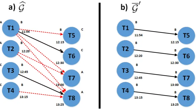
Fig. 1: On the left is represented a portion of Gb in location B, where those arcs in solid line represent the arcs inGand dashed line arcs denote those arcs chosen by LBH. On the right is the new G′ obtained which the fleet size is reduced.
in Figures 1a-b. In Figure 1a trip T1 links to T6 and T3 links to T8 (arcs in solid black line) while units for T2, T4 are no longer used and 2 units extra are required for T5 and T7. Hence, LBH builds Gbcollecting those potential arcs in dashed red line such as T1-T5, T2-T7, T3-T7 and T4-T8 and so on. In Figure 1b is presented the solution G′ where the two extra units were removed making a more efficient using of fleet.
Algorithm 2Location-Based-Heuristic
Require: µ,A,A¯,L
Ensure: H
1: M axArcs:=⌈µ· |AA|⌉¯
2: Arcs:= 0 3: for alll∈ Ldo
4: ArcsL:={l|a= (i, j) :id
=l′orjo =l′}
5: for alla∈ArcsLdo
6: if a /∈ Hthen
7: H:=H ∪ {a}
8: Arcs:=Arcs+ 1 9: end if
10: if Arcs≥M axArcs then
11: break
12: end if
13: end for
14: end for
Remark:
– Note thatL and ArcsLworks as a circular list. Since they retain the last point visited in order to explore the successive elements in other algorithm invocations and also starting from the first position when all positions are visited (lines 3 and 4) of Algorithm 2.
– Other important point considered here is that the locationsL are vis-ited in decreasingly order by the complexity (or number of arcs ). But in the case of the listArcsL, we tested two possibilities: arcs randomly sorted in the list (Rd), becoming more stochastic or sorted ascendency according to the arc slack time given byjd
t−i o
t thus deterministic (Ln).
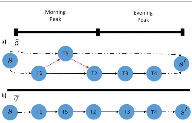
Fig. 2: Illustrative example of the THB works: on top is depicted the train horizon time splitted into 2 intervals. Below, two paths in a portion of G
where the solid arcs lines represent arcs inGand dashed black stand for sign-on/off whereas red ones denote the augmented arcsGbwhose arrival time is in the first interval. On the botton, is the resulted newG′ solved where the two paths become a one path.
Now all intervals are visited such that for each interval (lb, ub), the list of arcs ArcsLcontains those arcsa= (i, j), where the departure time jo
t of the trip j belong to the interval as is defined as below: ArcsL := {a = (i, j)|(lb, ub) : lb≤jo
t ≤ub}. Note that the THB algorithm is equivalent to Algorithm 2 but replacing lists LbyI also all points discussed in pre-vious section. In Figure 2a-b is depicted how TBH works. In 2a the thick black line on top denotes the time horizon which is divided into 2 intervals. The sub-graph below is formed by 2 paths (solid black lines and dashed black lines). This sub-graph represents an uneffiecient solutions because is required an extra train unit for covering T5 when it could be done by the same as path T1-T4. Hence, TBH is building the Gbwith pontencial arcs within in the first interval (dashed red line). In Figure 2b is presented the new solution G′ where the extra units was removed.
– PBH: Given a pathp∈G¯whose inward/outward arcs inA −A¯could po-tentially re-link the nodes ofpto a more efficient solution. This heuristic considers some of these arcs which are included in the set Hgiving rise to an enhancedG. The heuristic requires as input parameters two hash tables which given a nodei,SucN dL(i) return a list of inward arcs to nodeiand
maximum number of arcs per node.
Algorithm 3Path-Based-Heuristic
Require: µ,A,A,Pb, SucN dL, P reN dL, M axArcsN d
Ensure: H
1: M axArcs:=⌈µ· |A −A|⌉b
2: Arcs:= 0
3: whileArcs≤M axArcsdo
4: p:=ChooseRandomP ath(P) 5: for alli∈ nodes inpdo
6: ArcsN d:= 0
7: whileArcsN d≤M axArcsN dorArcs≤M axArcsdo
8: a:=P reN odeList(i).N ext() 9: a′:=SucN odeList(i).N ext()
10: if a /∈ Hthen
11: H:=H ∪ {a}
12: ArcsN d:=ArcsN d+ 1
13: Arcs:=Arcs+ 1 14: end if
15: if a′∈ H/ then
16: H:=H ∪ {a′}
17: ArcsN d:=ArcsN d+ 1
18: Arcs:=Arcs+ 1 19: end if
20: end while
21: end for
22: end while
In Algorithm 3 is presented the pseudo-code, the algorithm iterates until
M axArcs is not reached. In main loop a path p in chosen randomly, so for each node iuntil M axArcN darcs from the listsP reN odeList(i) and
SucN odeList(i) are included in the setH. Also listsP reN odeList(i) and
SucN odeList(i) are circular one.
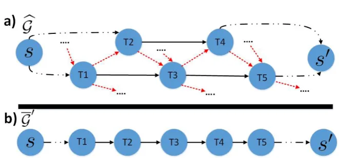
In Figures 3a and 3b is showed how PHB works: in Figure 3, there is a portion of G with two paths above (1) and below (2), the selected path is path (2), which solid and dashed black lines stand for arcs path and sign-on/off arcs, respectively. The Gb is constructed by arcs (dashed red) along the path (2). In Figure 3b, the newG′ path (1) and (2) became only one path reducing the fleet size in 1.
3.2.3 Concurrent Computing
Fig. 3: The PHB works as following: on top a portion of G with two paths above (1) and below (2), the selected path is path (2), which solid and dashed black lines stand for arcs path and sign-on/off arcs, respectively. The dashed red arcs along the path (2) are chosen forGb. On the bottom, path (1) and (2) became only one path reducing the fleet size in 1.
search to a cooperative multi-search where the same scheme is preserved: ex-traction, augmentation and solving, but running several RS-Opt at the same time.
Algorithm 4Multi-Thread SLIM (MTSLIM)
Require: . . . ,kmax
Ensure: G∗
1: L:=emptyList(lmax) 2: G0:=initialSolution(G)
3: L:=insertSorted( ¯G0, L)
4: while notendCriteriaReached(itmax, tmax, L)do 5: if notthreadAvailable(kmax)then
6: waitOne()
7: end if
8: runT hread(subP roblem(L)) 9: end while
Parameter Value
itmax 200
tmax 100000s
lmax 15
[image:13.595.72.413.187.274.2]µ 0.5
Table 1: SLIM input parameters for the heuristics comparison
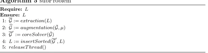
Algorithm 5subProblem
Require: L
Ensure: L
1: G:=extraction(L) 2: Gb:=augmentation( ¯G, µ) 3: G′:=coreSolver( ˆG) 4: L:=insertSorted(G′, L) 5: releaseT hread()
This new version of SLIM henceforth Multi-Thread SLIM (MTSLIM). MT-SLIM (Algorithms 4 and 5) differs from MT-SLIM (Algorithm 1) is the former requires a new input parameterkmax, which denotes number of threads. And also is necessary semaphores for synchronising threads and the main program in line 6 and line 5 in Algorithms 4 and 5 respectively. Note that ifkmax= 1 then MTSLIM becomes SLIM. In Section 4.2 is solved a small dataset.
4 Experiments
In the following sections we will present some of the result a we have obtained with the experiments. We will start with the outcomes from the Heuristic Assessment and compare them on each combination. Then we will present the results obtained from the concurrent computing and finally real-life cases.
4.1 Heuristics Assessment
The experiments carried out running 10 times setting SLIM with the pa-rameter tabled in Table 1. We ran SLIM with Location-based (Loc), Time-based (Tim) and Path-Time-based (Pth) separately. Each heuristic was run into two variats: in two variants: arcs sorted randomly (LocRd, TimRd, PthRd) or arcs sorted by slack time (deterministic LocLn, TimeLn).
LocRd LocLn TimRd TimLn PthRd LocRd+TimRd+PathRd
Bst Avg Bst Avg Bst Avg Bst Avg
[image:14.595.76.479.193.227.2]42.766 45.135 45.385 43.754 45.903 44.457 41.961∗ 43.911∗ 42.566 43.671∗
Table 2: Comparison of the heuristics solving a the same dataset
In Table 2 are shown the results for each heuristic and for stochastic heuris-tic is tabled the best of 10 result (Bst) and average (Avg). Other experiments carried out was the combination of all stochastic heuristics (LocRd+TimRd+PthRd in Table 2) according to this pattern λ ={L, T, P, L, T, P, P} where 50% of the iterations were used PthRd heuristic and with the same settings of Table 1.
As we can see highlighted in bold in Table 2 stochastic heuristics overcome deterministic ones . Besides, the PthRd was dominated over others as we ex-pected . The LocRd+TimRd+PthRd obtained the best average (highlighted in bold), however the PthRd was obtained the best performance of 10 runs. It seems that using all stochastic heuristics indicate that we can expect better results and the most frequent heuristic should be the PthRd inλ.
4.2 Concurrent computing
To compare the difference of these methods, we experimented with MTSLIM on the problem instance used in the previous section. The methods was con-figured with same parameters as well, with the exception of the parameter
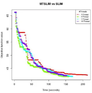
Fig. 4: : Comparison between SLIM (1-thread) against MTSLIM with 4-thread, 7-thread and 10-thread
In Figure 4 is ploted the average peformance of 10 runs of SLIM and MT-SLIM for eachkmax= 4,7,10. We can observe in Figure 4 that the MTSLIM for kmax > 1 converged to the optimal objective function value faster than SLIM. However, SLIM reached lower value than MTSLIM 7-threads (blue line) and 10-threads during the first 100 seconds. The configuration for MT-SLIM that get a better perfomance is 4-threads (green line) rather than 10 (purple line). The reason for that is that more than 4 threads running currently decreases the general algorithm efficiency for this dataset.
5 Real-life Cases
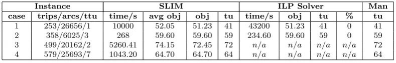
im-plemented SLIM in Visual C# 2017 and the ILP model was modelled using Xpress-Mosel language and solved by FICO Xpress 7.9. The experimental eval-uation was carried out on a PC with Intel(R) Core(TM) i7-4790 CPU with 2 cores at 3.60GHz and 32GB of RAM. For each case SLIM performed 10 run-ning attempts at maximum of 7200 seconds and 20 iterations except for the first instance which was 10000 seconds and 100 iterations. In both cases the so-lution list size was 10. Regarding to the initial soso-lution method FIFO was used in all cases except for cases 3 and 4 where theDC method and LP-relaxation was used respectively. The results given by SLIM are compared with the results obtained from running the ILP core solver alone with an optimality gap of 0% and with the manual schedules from the practitioners are displayed in Table 3.
Instance SLIM ILP Solver Man
case trips/arcs/ttu time/s avg obj obj tu time/s obj tu % tu
[image:16.595.70.465.252.315.2]1 253/26656/1 10000 52.05 51.23 41 43200 51.23 41 0 41 2 358/6025/3 268 59.60 59.60 59 234.60 59.60 59 0 59 3 499/20162/2 5260.41 74.15 72.45 72 n/a n/a n/a n/a 72 4 579/25693/7 1043.20 64.70 64.70 64 n/a n/a n/a n/a 64
Table 3: Comparison between SLIM, ILP model and Manual
The structure of the table is as follows. The first tow columns contain the configuration of each problem instance specified with the number of trips, number of arcs and number of train unit types (ttu). The next three columns provide the results of SLIM where the first column is the average time, the second is the average objective value and finally, the best objective value of the 10 runs and fleet size (tu). The next four columns show the results obtained by the ILP model with a maximum running time of 12h. In the cases that can be solved by the ILP solver, the objective value, fleet size and optimality gap are reported. The last column shows the manual results provided by practitioners.
It can be observed that SLIM can match almost the same quality as the human schedulers in terms of the fleet size. Moreover, the cost given by SLIM is very close to the theoretically best cost provided by the ILP model in those cases it can solve. In addition, SLIM can deal with some cases where the ILP solve alone cannot within the time limit.
6 Conclusions
heuristics for augmentation phase and an concurrent version which were as-sessed giving rise a suitable parameters settings. We achieved a high-quality solution in a reasonable time for many large sized instances. In future work, we will further consider different strategies for the extraction phase of selec-tion and replacement in the list of soluselec-tions, test MTSLIM/SLIM with other real-world cases, and tuning of parameters as well.
Acknowledgements This research is supported by an Engineering and Physical Sciences Council (EPSRC) project EP/M007243/1. We would like to also thank First Transpennine Express, First Great Western Railway, Abellio Group and Tracsis PLC for their kind and helpful collaboration.
References
Ahuja R, Magnanti T, Orlin J (1993) Network Flows: Theory, Algorithms, and Applications. DOI 10.1016/0166-218X(94)90171-6, URLhttp://cs.yazd. ac.ir/hasheminezhad/STSCS4R1.pdf
Cacchiani V, Caprara A, Toth P (2010) Scheduling extra freight trains on rail-way networks. Transportation Research Part B: Methodological 44(2):215– 231, DOI 10.1016/j.trb.2009.07.007, URLhttp://dx.doi.org/10.1016/j. trb.2009.07.007
Cacchiani V, Caprara A, Toth P (2013) A Lagrangian heuristic for a train-unit assignment problem. Discrete Applied Mathematics 161(12):1707–1718, DOI 10.1016/j.dam.2011.10.035, URL http://linkinghub.elsevier. com/retrieve/pii/S0166218X11004185
Chen J (2005) Confluent Flows. PhD thesis, Northeastern University
Copado-Mendez PJ, Lin Z, Kwan RS (2017) Size Limited Iterative Method (SLIM) for Train Unit Scheduling. In: Proceedings of the 12th Metaheuris-tics International Conference, Barcelona, Spain.(2017), Leeds
Lei L, Kwan RSK, Lin Z, Copado-Mendez PJ (2017) Station level refinement of train unit network flow schedules. In: 8th International Conference on Computational Logistics, ICCL 2017
Lin Z (2014) Passenger Train Unit Scheduling Optimisation. PhD thesis Lin Z, Kwan R (2014) A two-phase approach for real-world train unit
schedul-ing. Public Transport 6(1-2), DOI 10.1007/s12469-013-0073-9
Lin Z, Kwan RSK (2012) A Two-phase Approach for Real-world Train Unit Scheduling. Santiago, Chile, July, pp 23–27
Lin Z, Kwan RSK (2013) An integer fixed-charge multicommodity flow (FCMF) model for train unit scheduling. Electronic Notes in Discrete Math-ematics 41:165–172, DOI 10.1016/j.endm.2013.05.089, URL http://dx. doi.org/10.1016/j.endm.2013.05.089,arXiv:1011.1669v3
Lin Z, Kwan RSK (2017) Multicommodity Flow Problems with Commodity Compatibility Relations 00003, DOI 10.1051/itmconf/20171400003