Cosmic CARNage II: the evolution of the galaxy stellar
mass function in observations and galaxy formation models
Rachel Asquith,
1
?
Frazer R. Pearce,
1
Omar Almaini,
1
Alexander Knebe,
2,3
Violeta Gonzalez-Perez,
4,5
Andrew Benson,
6
Jeremy Blaizot,
7,8,9
Jorge Carretero,
10,11
Francisco J. Castander,
10
Andrea Cattaneo,
12
Sof´ıa A. Cora,
13,14
Darren J. Croton,
15
Julien E. Devriendt,
16
Fabio Fontanot,
17
Ignacio D. Gargiulo,
13,14
Will Hartley,
18
Bruno Henriques,
19
Jaehyun Lee,
20
Gary A. Mamon,
21
Julian Onions,
1
Nelson D. Padilla,
22,23
Chris Power,
24
Chaichalit Srisawat,
25
Adam R. H. Stevens,
15,24
Peter A. Thomas,
25
Cristian A. Vega-Mart´ınez,
13
Sukyoung K. Yi
26
1School of Physics & Astronomy, University of Nottingham, Nottingham NG7 2RD, UK
2Departamento de F´ısica Te´orica, M´odulo 15, Facultad de Ciencias, Universidad Aut´onoma de Madrid, 28049 Madrid, Spain 3Centro de Investigaci´on Avanzada en F´ısica Fundamental (CIAFF), Facultad de Ciencias, Universidad Aut´onoma de Madrid, 28049 Madrid, Spain
4Institute for Computational Cosmology, Department of Physics, University of Durham, South Road, Durham, DH1 3LE, UK 5Institute of Cosmology & Gravitation, University of Portsmouth, Dennis Sciama Building, Portsmouth, PO1 3FX, UK 6Carnegie Observatories, 813 Santa Barbara Street, Pasadena, CA 91101, USA
7Universit`e de Lyon, Lyon, F-69003, France
8Universit`e Lyon 1, Observatoire de Lyon, 9 avenue Charles Andr`e, Saint-Genis Laval, F-69230, France
9CNRS, UMR 5574, Centre de Recherche Astrophysique de Lyon ; Ecole Normale Sup`erieure de Lyon, Lyon, F-69007, France 10Institut de Ci`encies de l’Espai, IEEC-CSIC, Campus UAB, 08193 Bellaterra, Barcelona, Spain
11Port d’Informaci´o Cient´ıfica (PIC) Edifici D, Universitat Aut`onoma de Barcelona (UAB), E-08193 Bellaterra (Barcelona), Spain. 12GEPI, Observatoire de Paris, CNRS, 61, Avenue de l’Observatoire 75014, Paris France
13Instituto de Astrof´ısica de La Plata (CCT La Plata, CONICET, UNLP), Paseo del Bosque s/n, B1900FWA, La Plata, Argentina.
14Facultad de Ciencias Astron´omicas y Geof´ısicas, Universidad Nacional de La Plata, Paseo del Bosque s/n, B1900FWA, La Plata, Argentina 15Centre for Astrophysics and Supercomputing, Swinburne University of Technology, Hawthorn, Victoria 3122, Australia
16Astrophysics, University of Oxford, Denys Wilkinson Building, Keble Road, Oxford, OX1 3RH, UK 17INAF - Astronomical Observatory of Trieste, via Tiepolo 11, I-34143 Trieste, Italy
18Department of Physics and Astronomy, University College London, Gower Street, London WC1E 6BT 19Max-Planck-Institut f¨ur Astrophysik, Karl-Schwarzschild-Str. 1, 85741 Garching b. M¨unchen, Germany 20Korea Institute for Advanced Study, 85 Hoegiro Dongdaemun-gu, Seoul 02455 Korea
21Institut d’Astrophysique de Paris (UMR 7095: CNRS & UPMC), 98 bis Bd Arago, F-75014 Paris, France 22Instituto de Astrofisica, Universidad Catolica de Chile, Santiago, Chile
23Centro de Astro-Ingenieria, Universidad Catolica de Chile, Santiago, Chile
24International Centre for Radio Astronomy Research, University of Western Australia, 35 Stirling Highway, Crawley, Western Australia 6009, Australia
25Department of Physics & Astronomy, University of Sussex, Brighton, BN1 9QH, UK
26Department of Astronomy and Yonsei University Observatory, Yonsei University, 03722 Seoul, Republic of Korea
ABSTRACT
We present a comparison of the observed evolving galaxy stellar mass functions with the predictions of eight semi-analytic models and one halo occupation distribution model. While most models are able to fit the data at low redshift, some of them struggle to simultaneously fit observations at high redshift. We separate the galaxies into ‘passive’ and ‘star-forming’ classes and find that several of the models produce too many low-mass star-forming galaxies at high redshift compared to observations, in some cases by nearly a factor of 10 in the redshift range 2.5 < z <3.0. We also find important differences in the implied mass of the dark matter haloes the galaxies inhabit, by comparing with halo masses inferred from observations. Galaxies at high redshift in the models are in lower mass haloes than suggested by observations, and the star formation efficiency in low-mass haloes is higher than observed. We conclude that many of the models require a physical prescription that acts to dissociate the growth of low-mass galaxies from the growth of their dark matter haloes at high redshift.
Key words: methods:numerical – galaxies:haloes – galaxies: evolution – cosmol-ogy:theory – dark matter
1 INTRODUCTION
Locally, low-mass galaxies tend to be disky, blue and star-forming, whereas high-mass galaxies are more likely
to be spheroidal, red and passive (e.g. Kennicutt 1998;
Strateva et al. 2001; Kauffmann et al. 2003; Baldry et al. 2004). At high redshift (z > 1) we also observe this
bimodality in the galaxy population (Kovaˇc et al. 2014;
Cirasuolo et al. 2007), but do not definitively know the mechanisms by which these galaxies evolve into the popula-tions we observe locally. Various mechanisms have been sug-gested to move galaxies from the ‘blue cloud’ to the ‘red se-quence’ and shut off their star formation in a process known as ‘quenching’. Potential quenching mechanisms include en-vironmental effects and feedback from active galactic nuclei
(AGN) at high masses (for a review see Benson 2010), but
these processes are still not fully understood.
One way to study this problem is to directly observe galaxies forming and evolving in the distant Universe. At
high redshift (z > 1), deep near-infrared observations are
vital to select galaxies by rest-frame optical light. Selecting high-redshift galaxies using optical imaging will introduce strong biases against dusty galaxies or those with evolved
(i.e. passive) stellar populations (e.g. Cowie et al. 1996). It
is only recently that deep near-infrared surveys have been conducted with the required depth and area to produce large galaxy samples at high redshift, sufficient to allow accurate determinations of the galaxy stellar mass function while min-imising the influence of cosmic variance. In particular, the UKIDSS Ultra Deep Survey (UDS) (Lawrence et al. 2007, Almaini et al. in prep.) and UltraVISTA (McCracken et al. 2012) are now deep enough to detect typical (i.e.M∗)
galax-ies to z ∼ 3, over large volumes of the distant Universe
(∼100×100projected comoving Mpc atz=3). Using these
surveys, we can directly test model predictions for the build-up of the galaxy populations, rather than inferring their evo-lution by extrapolating back in time. However, each galaxy is only being seen at one point in its life and we cannot infer the full evolutionary history.
In order to get a cohesive picture of what happens to
? E-mail: [email protected]
galaxies throughout their lives, one approach is to link a population of galaxies at high redshift to a population at low redshift that could be their descendants. This can be done by selecting galaxies at a constant comoving number density when ranked by mass or luminosity (Mundy et al. 2015). This method was partly motivated by the need to overcome ‘progenitor bias’, where new young star-forming galaxies enter the sample at low redshift that are not present at high redshift (Shankar et al. 2015). Not accounting for this bias correctly can lead to a poor selection of the set of galaxies being connected as progenitor and descendent and therefore incorrect conclusions being drawn about their evolution.
A powerful method to trace galaxies through redshift is
to use semi-analytic models (SAMs) (for a review seeBenson
2010;Somerville & Dav´e 2015), a type of galaxy formation model in which simple analytic prescriptions (in connection with merger trees from either cosmological simulations or extended Press-Schechter formalisms) are used to model the physical processes occurring during galaxy formation and evolution. These models are able to evolve the same popula-tion of galaxies through redshift and connect them without the limitations of observational methods. These models are also computationally inexpensive, so can be used to simu-late large volumes and produce large catalogues of galaxies with which to compare observational data. By comparing the models to key observables, e.g. the evolution of the stel-lar mass function (SMF), we can learn about the physics of galaxy formation. If models are not able to reproduce ob-servational results it may mean that they are missing key physics which is important in galaxy formation and evolu-tion. Model galaxies can also be separated into ‘star-forming’ and ‘passive’ types, to test for the quenching processes which transform galaxies from star-forming to passive.
While it has been shown that SAMs are able to
re-produce the SMF at z = 0, they struggle to
simultane-ously match observations at both low and high redshift
(e.g.Fontanot et al. 2009;Weinmann et al. 2012;Guo et al.
galaxies form earlier with their abundance changing little
fromz∼1to the present day, whereas there is a rapid
evo-lution in the number of low-mass galaxies at late times (e.g. Fontana et al. 2004,2006;Faber et al. 2007;Pozzetti et al. 2007; Marchesini et al. 2009, 2010; Pozzetti et al. 2010; Ilbert et al. 2010, 2013;Muzzin et al. 2013). This is some-times referred to as ‘mass assembly downsizing’ (Cowie et al. 1996;Cimatti et al. 2006;Lee & Yi 2013).
After much work understanding both AGN feed-back and the mass assembly of high-mass galaxies (e.g. Benson et al. 2003; Di Matteo et al. 2005; Bower et al. 2006;Croton et al. 2006), models are now able to reproduce the high-mass end of the galaxy stellar mass function over a range of redshifts. However, models still typically overpro-duce the number of low-mass galaxies at high redshift. The main reason for this discrepancy appears to be that galaxies in the models follow the growth of their dark matter haloes
too closely (Weinmann et al. 2012;Somerville & Dav´e 2015;
Guo et al. 2016). Halo mass growth is the main driver of gas accretion rate in galaxies, which then in turn drives the star formation rate. The star formation history then traces the dark matter mass accretion history, which, in the favoured
ΛCDM structure formation scenario, is approximately
self-similar for haloes of different masses. However, in the real Universe it appears that there is not such a tight correlation
(White et al. 2015;Guo et al. 2016).
This excess of low-mass galaxies at high redshift was
investigated by Fontanot et al. (2009), who found that in
three different SAMs, galaxies in the mass range 9 <
log(M∗/M)<11form too early and have little ongoing star
formation at late times. They concluded that the physical processes operating on these mass scales, such as supernova
feedback, needed a re-think. Weinmann et al. (2012) later
used two SAMs and two cosmological hydrodynamical sim-ulations and examined the evolution of the observed number density of galaxies. They found that although the models fit
well at z = 0, the low-mass galaxies were formed at early
times. They conclude that as the current form of feedback is mainly dependent on host halo mass and time, it is un-likely to be able to separate the growth of galaxies from the growth of their dark matter haloes.
Monte Carlo Markov Chain (MCMC) methods were
used by Henriques et al. (2013) in an attempt to fit the
stellar mass function at all redshifts, but they could not find a single set of parameters that allowed this. They then changed the reincorporation timescale for ejected gas to be inversely proportional to halo mass and independent of red-shift and found that they were able to fit observed numbers
of low-mass galaxies from 0< z <3. However, the passive
fraction of low-mass galaxies was still too high. Their model
was later updated further inHenriques et al. (2015) where
they also reduce ram-pressure stripping in low-mass haloes, make radio-mode AGN feedback more efficient at low red-shift, and reduce the gas surface density threshold for star formation. They then find that their model reproduces the observed abundance and passive fraction of low-mass galax-ies, both at high and low redshift.
Another attempt to solve this problem was by
White et al.(2015), who tried three different physically mo-tivated methods to decouple the accretion rate in galaxies from their star formation rate. They found that changing the gas accretion to be less efficient in low-mass haloes at early
times and increasing the dependence of stellar feedback on halo mass at high redshift were the most successful at qual-itatively matching the evolution of the number density of low-mass galaxies. However, they allow these functions to scale with halo mass and redshift in an arbitrary way which
may not be physically motivated.Hirschmann et al.(2016)
also investigated this problem with their model and found that they improved their agreement with observations by ei-ther reducing the gas ejection rate with cosmic time or vary-ing the reincorporation timescale with halo mass, classed as ‘ejective’ and ‘preventative’ feedback schemes respectively. Although their results improve from their fiducial model, they still find too many low-mass, red, old galaxies between 0.5<z<2.0.
However, the effect of adjusting certain physical prescriptions can be vastly different between models. White et al.(2015) investigated what effect replicating the
changes inHenriques et al.(2013) had on their own model,
but found that it did not make much difference to the ob-served number density of low-mass galaxies. They conclude that this is due to the sensitivity of the results to how the gas reservoirs are tracked and treated in the different codes. Croton et al.(2016) also had similar problems with this ap-proach and found that it did not solve the problems with fitting the stellar mass function. This presents difficulties to the modelling community, as it means that different mod-els may require different changes to get them to match the observed evolution.
It is also possible to try and match the galaxy stellar mass function at all redshifts without changing the physics
involved in the model. For example,Rodrigues et al.(2017)
usedGalformto identify a small region of parameter space
where the model matched the observational data out toz=
1.5, without needing to adapt any of the physics involved.
They found that the parameters controlling the feedback processes were most strongly constrained, suggesting that these processes are important when fitting the evolution of the galaxy stellar mass function.
Halo occupation distribution (HOD) models, rather than modelling the physical processes that we think go into galaxy formation, use statistical methods to match galaxies to their corresponding dark matter haloes (e.g. Berlind & Weinberg 2002;Zheng et al. 2005). As these mod-els are applied independently at each redshift, the evolution of each galaxy is not tracked, although they can be con-nected to their progenitors and descendants via dark matter merger trees. HOD models by design are able to reproduce the SMF at each redshift and are therefore able to repro-duce the population of galaxies at any given time. This type of model is a very useful tool for learning about the rela-tionship between galaxies and their host dark matter haloes and how this changes as a function of redshift. For example, Berlind et al.(2003) found that low-mass haloes are mainly populated by young galaxies and high-mass haloes by older galaxies.
Galaxy formation models such as HODs and SAMs must be calibrated using observational datasets. Varying the
calibration dataset,even for the same modelmay produce
of the required physics or that the underlying observational datasets are incomplete or are physically incompatible with each other.
In the Cosmic CARNage mock galaxy comparison project (Knebe et al. 2018, hereafter referred to as Paper I) we sought to address some of these issues by requiring the participants to calibrate their models to the same set of observational data. These data included the galaxy stellar
mass function at z =0 and z =2, the star formation rate
function at z =0.15, the black-hole bulge-mass relation at
z=0, and the cold gas mass fraction at z=0. Participants
were free to weight these five calibrations as they saw fit, and were asked to generate their “best-fit” model that took all of them into account, i.e. calibration set ‘-c02’ in Paper I.
We will build on previous work by investigating the evo-lution of the SMF for the eight SAMs and one HOD model that were used in Paper I. These models are all calibrated to the same observational data and are all run on the same background dark matter only simulation, which means that we can discount the differences due to the underlying cosmo-logical framework when considering the differences between the models. Our aim is then to see if the current physical prescriptions used in any of the galaxy formation models can produce a realistic population of galaxies at both low and high redshift. We will investigate the evolution of the SMF in
the redshift range0.5<z<3.0for all nine galaxy formation
models and determine if models still struggle to simultane-ously match observations both at low and high redshift.
The rest of this paper is structured as follows: in Section
2we will briefly explain the underlying dark matter
simula-tion and the parameters used. In Secsimula-tion 3we will present
the results for the evolution of the SMF and the passive frac-tion. We will then show how the specific star formation rate of star-forming galaxies in the models evolves. We will also examine the average halo mass as a function of stellar mass and the stellar mass - halo mass relation for all the models.
In Section4we will present our discussion and in Section5
we will present our conclusions.
2 SIMULATION DATA
The eight SAMs we will be using are
DLB07 (De Lucia & Blaizot 2007), Galform
(Gonzalez-Perez et al. 2014), GalICS-2.0 (Cattaneo et al.
2017, although the exact version used for this comparison
is the one described in the appendix of Knebe et al.
(2015)), Lgalaxies (Henriques et al. 2013), Morgana
(Monaco et al. 2007), Sag (Cora et al. 2018), Sage
(Croton et al. 2016) and ySAM (Lee & Yi 2013). The
single HOD model is Mice (Carretero et al. 2015). A
brief description of the physical prescriptions used in each
model is given in the Appendix ofKnebe et al.(2015). Any
changes to any of the models since then are included in
AppendixA.
The models have all been run on the same underlying dark matter simulation which may be different to the one used in the above reference papers. This can lead to changes in the predictions of each model, as can varying the initial mass function, yield, stellar population synthesis model and calibration data set used.
A description of how the models were calibrated to the same observational data is given in Paper I. We also note that the stellar masses from the models have been convolved
with a0.08(1+z)dex scatter to account for the observational
errors when measuring stellar mass. This value comes from Conroy et al.(2009), who estimate an error of∼0.2dex at
z=2when fixing the stellar population synthesis model.
The underlying cosmological dark-matter-only
simula-tion was run using the Gadget-3 N-body code (Springel
2005) with parameters given by the Planck cosmology
(Planck Collaboration et al. 2014,Ωm =0.307,ΩΛ =0.693,
Ωb = 0.048, σ8 = 0.829, h = 0.677, ns = 0.96).
We use 5123 particles of mass 1.24 × 10⁹h−1M in a
box of comoving width 125h−1Mpc. The halo catalogues
were extracted from 125 snapshots and identified using
Rockstar (Behroozi et al. 2013a). The halo merger trees
were then generated using the ConsistentTrees code
(Behroozi et al. 2013b).
3 RESULTS
3.1 Evolution of the Galaxy Stellar Mass Function
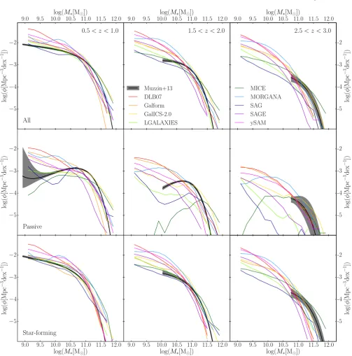
We start by examining the evolution of the stellar mass
func-tion in Figure1, shown for the whole sample in the top row.
The coloured lines are the stellar mass functions for each of the models, computed for each redshift bin using single
snap-shots atz=0.8,2.0and3.0for each redshift bin respectively.
We note that the precise choice of snapshot does not
af-fect our conclusions. The observations fromDavidzon et al.
(2017) are based on the UltraVISTA near-infrared survey of the COSMOS field and are shown as a black line and dark shaded region. When finding the best-fit Schechter param-eters to their stellar mass functions, they take into account the errors in measuring stellar mass, known as Eddington bias. As they have applied this correction, when plotting
the stellar mass function we do not apply the0.08(1+z)dex
scatter to the stellar mass values. In AppendixBwe have
in-cluded a version of Figure1where the model stellar masses
do have this scatter applied, to show the differences to the SMF.
We also note that we compare to different observational data than the combined dataset used to calibrate the models.
The data from Davidzon et al.(2017) is more recent than
the calibration dataset and also allows us to split our sam-ple into passive and star-forming galaxies. When comparing Davidzon et al.(2017) to the stellar mass function
calibra-tion data atz=0andz=2, the two largely agree, although
the former has smaller error bars. This is encouraging as it shows good agreement between different observations.
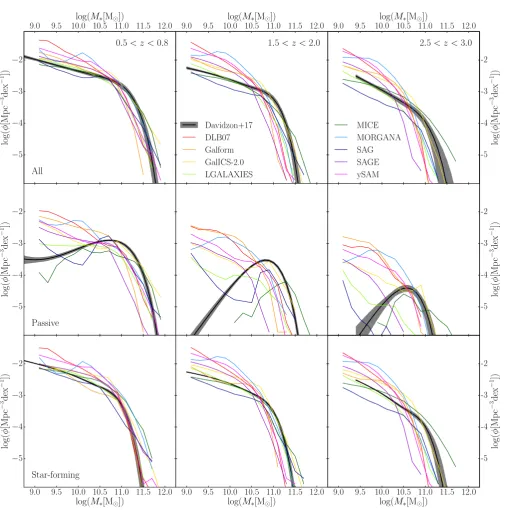
Inspecting the top panels, what is clear is that the ob-servational number counts are evolving, with the high-mass
end largely in place byz=3, while the low-mass end rises at
late times. Whilst the models match the observations well at low redshift, the strong evolution at the low-mass end is not seen for most of the galaxy formation models. The
excep-tions to this areMice,LgalaxiesandSag, which all show
an increasing number density of low-mass galaxies towards
low redshift. AsMiceis an HOD model it has been designed
to match the evolution of the SMF. Lgalaxies and Sag
−5
−4
−3
−2
log
(
φ
[Mp
c
−
3 dex
−
1 ])
0.5< z <0.8
All
1.5< z <2.0
Davidzon+17 DLB07 Galform GalICS-2.0 LGALAXIES
2.5< z <3.0
MICE MORGANA SAG SAGE ySAM
−5
−4
−3
−2
log
(
φ
[Mp
c
−
3 dex
−
1 ])
Passive
9.0 9.5 10.0 10.5 11.0 11.5 12.0
log(M∗[M])
−5
−4
−3
−2
log
(
φ
[Mp
c
−
3 dex
−
1 ])
Star-forming
9.0 9.5 10.0 10.5 11.0 11.5 12.0
log(M∗[M])
9.0 9.5 10.0 10.5 11.0 11.5 12.0
log(M∗[M])
9.0 9.5 10.0 10.5 11.0 11.5 12.0log(M∗[M]) 9.0 9.5 10.0 10.5 11.0 11.5 12.0log(M∗[M]) 9.0 9.5 10.0 10.5 11.0 11.5 12.0log(M∗[M])
-5 -4 -3 -2
log
(
φ
[Mp
c
−
3dex
−
1 ])
-5 -4 -3 -2
log
(
φ
[Mp
c
−
3dex
−
1 ])
-5 -4 -3 -2
log
(
φ
[Mp
c
−
3dex
−
[image:5.595.43.549.89.600.2]1 ])
Figure 1.The evolution of the stellar mass function for all the models over the range0.5<z <3.0. The stellar mass function for the whole, passive and star-forming samples are shown in the top, middle and bottom panels, respectively, as coloured lines. The black line is the observational best-fit mass functions fromDavidzon et al. (2017), with the dark grey shaded region showing the1σ errors. For the models, each redshift bin contains one snapshot, at redshiftsz =0.8,2.0and3.0respectively. We can see that the models match well at low redshift (by construction), but deviate further from the observations at high redshift. The number density of the lowest mass objects is nearly constant in the models but changes by more than0.5dex in the observations. Most of the low-mass galaxies that are not present in the observations at high redshift seem to be star-forming.
due to the physics involved in the treatment of gas. Both
follow the prescription suggested inHenriques et al.(2013)
of scaling the reincorporation timescale of ejected gas with the inverse of the halo mass. This means the process of gas being reincorpoated back into the halo takes longer for low-mass haloes, shifting the growth of galaxies in these haloes
from early to late times.Sag also scales the reheated and
ejected mass with redshift to make supernova feedback more efficient at high redshift.
At the high-mass end, the models underestimate the
number density compared to observations, with Miceand
GalICS-2.0 as the exceptions. One alternative reason
9.0 9.5 10.0 10.5 11.0 11.5 12.0
log(M∗[M])
0.0
0.2
0.4
0.6
0.8
1.0
P
assiv
e
fraction
0.5< z <0.8
Davidzon+17 DLB07 Galform
9.0 9.5 10.0 10.5 11.0 11.5 12.0
log(M∗[M])
1.5< z <2.0
GalICS-2.0 LGALAXIES MICE
9.0 9.5 10.0 10.5 11.0 11.5 12.0
log(M∗[M])
2.5< z <3.0
MORGANA SAG SAGE ySAM
0.0 0.2 0.4 0.6 0.8 1.0
P
assiv
e
[image:6.595.42.546.79.276.2]fraction
Figure 2.The evolution of the passive fraction over the range0.5<z<3.0. The coloured lines, black solid lines and grey shaded regions are the same as in Figure1, as are the snapshots used in each redshift bin for the models. For a few models the passive fraction is too high at low masses, particularly at low redshift. The models match well at high masses at low redshift, but generally underpredict the passive fraction for high-mass galaxies at high redshift.
9.0 9.5 10.0 10.5 11.0 11.5 12.0
log(M∗[M])
−2.5 −2.0 −1.5 −1.0 −0.5
log
(sSFR[Gyr
−
1])
Elbaz+07 DLB07 Galform GalICS-2.0 LGALAXIES MICE MORGANA SAG SAGE ySAM
[image:6.595.42.283.338.571.2]z= 0.0
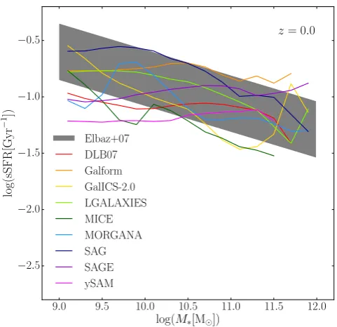
Figure 3.The relationship between mass and sSFR atz=0.0for star-forming galaxies in the nine models. The model data is taken from one snapshot at z =0.0. The grey shaded region is taken
fromElbaz et al.(2007) and shows the observational best-fit to
this relation. The sSFR of star-forming galaxies in the models matches observations well but there is less of a trend with mass in some models.
when accounting for Eddington bias, as it is very difficult to accurately measure all of the sources of error. Due to the steep slope of the SMF at high masses this would have a greater impact at the high-mass end of the SMF. The im-pact of Eddington bias on the SMF are discussed further in
AppendixB.
9.0 9.5 10.0 10.5 11.0 11.5 12.0
log(M∗[M])
−2.5 −2.0 −1.5 −1.0 −0.5
log
(sSFR[Gyr
−
1 ])
Elbaz+07 DLB07 Galform GalICS-2.0 LGALAXIES MICE MORGANA SAG SAGE ySAM
z= 0.0
Figure 4.As for Figure3, but forz=2.0and observations from
Daddi et al.(2007). The model data is taken from one snapshot
atz=2.0. Here all of the models lie almost completely below the observational best-fit range.
3.2 Star-forming and Passive Galaxy Stellar Mass Functions
We explore the mass growth further in the bottom two rows
of Figure 1, splitting the population into passive (middle
row) and star-forming (bottom row) galaxies. We separate passive and star-forming galaxies using a redshift-dependent
specific star formation rate (sSFR) cut of sSFR(z) =
1/(3tH(z)) where tH(z) is the Hubble time at that
red-shift. We test the robustness of this cut by examining the change in our results when using slightly different cuts of
sSFR(z)=1/(2tH(z))andsSFR(z)=1/(4tH(z)). We find that
[image:6.595.301.546.339.571.2]−1.5 −1.0 −0.5 0.0
log
(
φ/φ
0
)
9<log(M∗[M])<10
All
Davidzon+17 DLB07 Galform GalICS-2.0
−2.5 −2.0 −1.5 −1.0 −0.5 0.0 0.5
log
(
φ/φ
0
)
Passive
0.5 1.0 1.5 2.0 2.5 3.0 z
−1.0 −0.5 0.0 0.5
log
(
φ/φ
0
)
Star-forming
10<log(M∗[M])<11
LGALAXIES MICE MORGANA
0.5 1.0 1.5 2.0 2.5 3.0 z
11<log(M∗[M])<12
SAG SAGE ySAM
0.5 1.0 1.5 2.0 2.5 3.0 z
2 4 6 8 tlb10[Gyr] 11 2 4 6 8 tlb[Gyr]10 11 2 4 6 8 tlb10[Gyr] 11
-1.5 -1.0 -0.5 0.0
log
(
φ/φ
0
)
-2.5 -2.0 -1.5 -1.0 -0.5 0.0 0.5
log
(
φ/φ
0
)
-1.0 -0.5 0.0 0.5
log
(
φ/φ
0
[image:7.595.44.546.85.586.2])
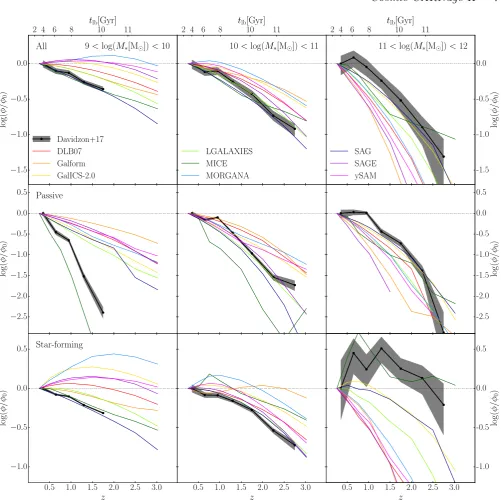
Figure 5.The evolution of the number densityφ, in bins of stellar mass. This is normalised by the number density at0.2<z <0.5, which we callφ0. We show three mass bins as indicated (left to right panels) for all galaxies (top panels), passive galaxies (middle panels) and star-forming galaxies (bottom panels). The dark grey shaded regions and black lines with circular points show data from
Davidzon et al.(2017). The coloured points and lines are for the nine models. In the lowest mass bin, most of the models assemble the
galaxies before the observations. The models match the observations well at intermediate masses, but the observational number density increases before many of the models at high mass.
makes no difference to any of the conclusions that we draw. In the observations the passive and star-forming galaxies are seperated using the (NUV - r) vs (r - J) colour-colour
diagram as described in Ilbert et al. (2013), which is best
suited to differentiate fully quiescent galaxies from those with residual star formation. In practice, the exact location of the split makes little difference to the low-mass end of the star-forming SMF and the high-mass end of the passive
SMF, as these galaxies will have very blue and red colours respectively.
Splitting the galaxy population in this way reveals that the main source of the difference between the observations and the models comes from the star-forming population: low-mass star-forming galaxies appear to be far too com-mon at high redshift in the models and the star-forming
SMF evolves little fromz=3to z=0.5. The exceptions to
11.5 12.0 12.5 13.0 13.5 14.0 14.5
log
(
M200 [M
])
0.5< z <1.0
All Baryon fraction 1.0< z <2.0
Hartley+13 DLB07 Galform GalICS-2.0 LGALAXIES
2.0< z <3.6
MICE MORGANA SAG SAGE ySAM
11.5 12.0 12.5 13.0 13.5 14.0 14.5
log
(
M200 [M
])
Passive
9.0 9.5 10.0 10.5 11.0 11.5 12.0
log(M∗[M])
11.5 12.0 12.5 13.0 13.5 14.0 14.5
log
(
M
200
[M
])
Star-forming
9.0 9.5 10.0 10.5 11.0 11.5 12.0
log(M∗[M])
9.0 9.5 10.0 10.5 11.0 11.5 12.0
log(M∗[M])
9.0 9.5 10.0 10.5 11.0 11.5 12.0
log(M∗[M])
9.0 9.5 10.0 10.5 11.0 11.5 12.0
log(M∗[M])
9.0 9.5 10.0 10.5 11.0 11.5 12.0
log(M∗[M])
11.5 12.0 12.5 13.0 13.5 14.0 14.5
log
(
M200 [M
])
11.5 12.0 12.5 13.0 13.5 14.0 14.5
log
(
M200 [M
])
11.5 12.0 12.5 13.0 13.5 14.0 14.5
log
(
M
200
[M
[image:8.595.43.545.89.586.2]
])
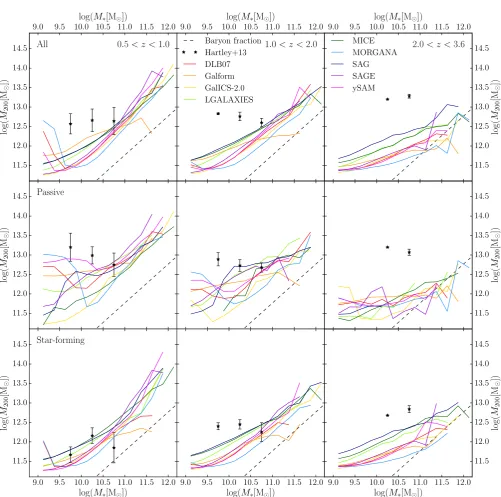
Figure 6.The average halo mass in the models compared to measurements from observations betweenz=0.5andz=3.6. Observational measurements of the average halo mass from Hartley et al.(2013) are derived from clustering and are shown as stars. The values for each model are shown as coloured lines. For the models, the mass of the main host halo was used rather than the subhalo, to better compare with observational halo mass measurements from clustering. The top panels cover the full galaxy sample, the middle panels are for passive galaxies and the bottom panels are for star-forming galaxies. The black dashed line shows the universal baryon fraction. For the models, we use snapshots atz=1.0,2.0and3.5for each redshift bin respectively. For the passive sample, the halo masses from observations are approximately constant, but decrease by up to a factor of 10 in the models with increasing redshift. For the star-forming sample, the observations show halo mass increasing with increasing redshift, whereas in the models there is no real trend with redshift.
the observations at low masses up toz=3. For the passive
galaxies, the number density at low masses does evolve with redshift in the models, as seen in the observations. However, most of the SAMs show rising number density towards lower masses, in contrast with the observations which appear to show a turnover or flattening of the passive SMF towards lower masses. In order to solve these problems, models need
11.0 11.5 12.0 12.5 13.0 13.5 14.0 14.5
log(M200[M])
9.5 10.0 10.5 11.0 11.5 12.0
log
(
M∗
[M
])
z= 0.1
Behroozi+13 Baryon fraction DLB07 Galform
11.0 11.5 12.0 12.5 13.0 13.5 14.0 14.5
log(M200[M])
z = 1.0
GalICS-2.0 LGALAXIES MICE MORGANA
11.0 11.5 12.0 12.5 13.0 13.5 14.0 14.5
log(M200[M])
z= 2.0
SAG SAGE ySAM 9.5
10.0 10.5 11.0 11.5 12.0
log
(
M∗
[M
[image:9.595.47.545.81.273.2]
])
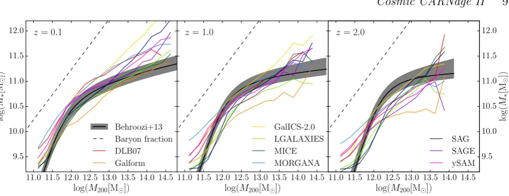
Figure 7.Comparison of the average stellar mass for each halo mass bin in the models to the abundance matching model ofBehroozi et al.
(2013c), considering only central galaxies. The results from the models are shown as coloured lines and the stellar mass - halo mass
relation fromBehroozi et al.(2013c) is shown as a dark grey shaded region and black line. The black dashed line shows the universal baryon fraction. The panels are for each redshift, increasing from left to right, using snapshots atz=0.0,1.0and2.0respectively. Looking at the data fromBehroozi et al.(2013c), we can see that the average stellar mass stays fairly constant with redshift, but increases in the models towards low redshift, particularly at high masses.
3.3 Evolution of the Passive Fraction
Another way of looking at this result is to examine the
pas-sive fraction, which is shown in Figure2. Again, the shaded
regions indicate the observations taken from the same source
as used for Figure1. The passive fraction indicates the ratio
of passive to star-forming galaxies. At low masses, some of
the models, such asDLB07,GalformandMorgana, tend
to overestimate the passive fraction compared to observa-tions. This has been seen previously and appears to be linked to how environmental processes are taken into account in
the models (Lagos et al. 2014;Gonzalez-Perez et al. 2018).
At low redshift the number of star-forming galaxies matches observations well, so this difference is due to the lack of a turnover or flattening of the passive SMF. At higher red-shifts, the overproduction of low-mass star-forming galaxies would act to decrease the passive fractions. However, this is still too high in some models, again due to the rising number density towards low masses in the passive SMF.
At low redshift, the models tend to match the
observa-tions well at high masses, but one model,Sage,
underpre-dicts the passive fraction. This is mainly due to an under-prediction for the number of high-mass passive galaxies. As
shown byStevens & Brown(2017), detailing the structural
evolution of galaxy discs with the Dark Sage variant of
the model (Stevens et al. 2016) leads to more sensible
pas-sive fractions. In the redshift range1.5< z<2.0the
mod-els tend to underpredict the fraction of high-mass galaxies, mainly due to the lack of high-mass passive galaxies above
z∼1. The model which best matches the observed passive
fraction for high-mass galaxies isDLB07, which slightly
un-derpredicts the number density of both high-mass passive and star-forming galaxies in this redshift range.
3.4 Relationship between Mass and Specific Star Formation Rate
In order to better compare star formation in the observations and the models, we also look at the specific star formation
rates of the subset of star-forming galaxies. Figure3shows
the average sSFR as a function of mass atz=0.0for each of
the models as a solid coloured line. The grey shaded region is
taken fromElbaz et al.(2007), who used SDSS data to find
a fit to the correlation between SFR and mass atz=0. Their
sample is made up of 19590 galaxies with redshiftsz=0.04−
0.1and is complete toMB≤ −20.Brinchmann et al.(2004)
usedHα emission to derive the SFR of these galaxies and
the stellar masses were derived byKauffmann et al.(2003),
who fit using a library of star formation histories to find the most likely stellar mass.
Most of the models match the observations well here,
withLgalaxiesandSaglying in the observational region
at all masses. Some models appear to evolve less with mass than the observations suggest, with some showing almost no trend, whereas the sSFR implied by the observations
de-creases by over 0.5 dex between109M and1012M. This
means that some of the models, such asGalform, match at
low masses but not high masses, and others such asDLB07
andySAMmatch at high masses but not low masses. This
was also discussed inGuo et al.(2016), who used data from
two SAMs, Galform and Lgalaxies, and one
hydrody-namical simulation, Eagle. They found that the median
sSFR remained almost constant with mass, in contrast with observations.
The relationship between sSFR and stellar mass atz=
2.0is then shown in Figure4. Here the observations are taken
fromDaddi et al.(2007), who use galaxies in the GOODS-S
field to find the correlation between SFR and mass atz=2.
They are complete to K <22 and use only 24µm selected
galaxies in order to exclude passive galaxies. The SFRs were estimated using the UV and the stellar masses were derived byFontana et al.(2004) using SED fitting.
The models therefore predict a slower evolution of the sSFR with redshift than observations. This has been previously
seen byMitchell et al.(2014), who find that when they scale
the reincorporation time of gas with redshift they are able to better match the evolution of the stellar mass function, but still underestimate the sSFR of high-mass galaxies at z ∼2. Hirschmann et al. (2016) also found that their ejec-tive models predicted lower than observed sSFRs at high redshift, even when they could reproduce the growth of the stellar mass function.
Reducing the star formation rates of galaxies abovez∼
2, as suggested in Section3.2, may help to solve this problem.
If galaxies have a lower star formation rate at higher redshift, their resulting mass at lower redshift will be lower. A galaxy
with the same star-formation rate atz=2will then have a
higher sSFR as it will have a lower stellar mass.
3.5 Growth of the Galaxy Stellar Mass Function
In Figure5we examine the growth of the stellar mass
func-tion as a funcfunc-tion of mass and redshift. This is found by
taking the value of the number density φ at fixed stellar
mass for a certain redshift bin and normalising it by the
value of φ in the lowest redshift bin 0.2 < z < 0.5, which
we call φ0. This allows for easier comparison between the
models and observations and will highlight when the num-ber density of different populations increases. The dark grey region and black line with circular points shows data from Davidzon et al. (2017). The coloured lines then show the number density evolution for the nine models. The black dotted line shows where the number density is equal to the number density in the lowest redshift bin.
Looking at the passive galaxies, we can see that the models struggle to match the observed growth of the mass function at low masses, as the number density of low-mass galaxies increases in the models at higher redshift than the
observations. The only exception is Mice, which has very
few galaxies with mass below 1010M above z ∼1. At
in-termediate masses the models match the observations well, but at high masses the growth of the mass function occurs in observations before many of the models.
For the star-forming galaxies, at low masses there is a similar problem with several of the models; the mass func-tion grows too much at high redshift. Just under half of the models have more low-mass star-forming objects in the highest redshift bin than the lowest redshift one. However, several of the models are more in line with the growth of the
observed mass function, namelySagandMice. At
interme-diate masses, the number density of star-forming galaxies increases at higher redshift in the models than in the
ob-servations. The model that is most discrepant, Morgana,
has more intermediate mass star-forming galaxies between
1.0<z <1.5than in the lowest redshift bin. For high-mass
galaxies, the number density evolves little since high
red-shift in the observations. Mice reproduces this trend well
but in other models the number density increases at lower redshift. This may be in part due to the fact that there are low numbers of the highest mass galaxies which will natu-rally introduce more scatter in the proportional change in number density.
We can also see interesting differences between mod-els when comparing the stellar mass function to the growth
of the stellar mass function. Looking at the lower panel of
Figure 1, we can see that DLB07 overpredicts the
num-ber of low-mass star-forming galaxies at both low and high
redshift.Sageagrees well with observations at low redshift
but overproduces low-mass star-forming galaxies at high
red-shift. However, looking at the lower left panel of Figure5,
we can see thatDLB07matches observations of the growth
of the mass function better thanSage. These models
there-fore have slightly different problems;DLB07has too many
low-mass galaxies at all redshifts, but the number density
in-creases at the correct rate. Conversely,Sagehas the correct
number at low redshift, but the number density increases too early.
3.6 Average Halo Mass
In this section we study the average halo mass the
galax-ies reside within, shown in Figure6. For the models we use
single snapshots at z=1.0,2.0and 3.5for each redshift bin
respectively. The dashed black line indicates the universal baryon fraction, i.e. where all the baryonic material within the halo has been converted into stars. Each of the coloured lines indicates the average halo mass values for a different model, while the black points with errorbars are average
halo mass values taken fromHartley et al.(2013), who use
the UDS DR8 data to estimate the halo masses from
mea-surements of galaxy clustering (e.g.Mo & White 2002, and
references therein).
For the models, here we use the mass of the main host halo for each galaxy rather than the mass of its subhalo. Host haloes do not reside within another halo, whereas subhaloes are contained within a host halo. Although us-ing the host halo is not necessarily the usual choice when analysing simulation data, it allows us to compare to obser-vational measurements of halo mass from galaxy clustering, which effectively measure the mass of the main host haloes (Mo & White 2002). For this reason we also include both centrals and satellites, in order to best mimic the observa-tional measurements. Assuming galaxy clustering measure-ments can correctly recover the host halo mass, we can then directly compare the observations and models.
Splitting the sample into passive and star-forming
galaxies in Figure 6 we see that there are marked
differ-ences between the observations and the models. For passive galaxies, the average halo mass in observations stays con-stant over redshift in the observations, but rises towards low redshift in the models. For the star-forming population, while the observations indicate a general downsizing trend in halo mass of about an order of magnitude between high and low redshift, all the models show virtually no change. It is clear that the models start significantly below the
observa-tions at2.0<z <3.5and only agree with the observations
by0.5< z <1.0. Both passive and star-forming low-mass
galaxies are therefore in lower mass haloes on average in the models than in the observations at high redshift.
clus-tering is ‘halo assembly bias’, which refers to the fact that halo clustering can depend on other properties besides halo
mass. For example, Gao et al. (2005) found that at fixed
halo mass, haloes that assembled earlier are more clustered than those that assembled later. Therefore, galaxies in older haloes will be more strongly clustered than they should be for their halo mass, which means that their halo masses will be measured as higher than they actually are. This could alleviate some of the discrepancy between the observations and models. For example, if the passive galaxies observed at low redshift are associated to older haloes, then their halo masses could have been overestimated.
3.7 Stellar Mass - Halo Mass Relation
In Figure 7 we display measurements of the average
stel-lar mass of central galaxies in bins of halo mass, com-paring the models with the abundance matching model of Behroozi et al.(2013c). The dashed black line indicates the universal baryon fraction and the dark grey region and black solid line show the fit to the stellar mass - halo mass
(SMHM) relation fromBehroozi et al.(2013c). The coloured
lines show the average stellar mass values for each different model.
At low redshift, the results from the models and SMHM relation agree well at low and intermediate halo masses.
However, above halo masses of∼1013.5Mthe average
stel-lar mass of centrals in the models is higher than suggested by the SMHM relation. This means that at low redshift, star formation in high-mass haloes is more efficient in the
mod-els. The exceptions to this areLgalaxiesandMice, which
agree with the SMHM relation at nearly all halo masses. For most of the models, the slope of the relation at high halo masses does flatten, but not to the extent seen from the SMHM relation.
As we move to higher redshift the SMHM relation changes little. The peak of the relation moves to slightly higher halo masses and the average stellar mass for low-mass
haloes decreases by ∼ 0.4 dex at 1011.5M. In the
mod-els the average stellar mass for low-mass haloes decreases slightly with increasing redshift, but is above the SMHM
relation by z =1.0for most models. This discrepancy can
be partially explained by the cut in stellar mass applied
at M∗ = 109Mh−1, which may have skewed the
distribu-tion towards higher stellar masses. This might be enough
to explain the difference for models such as Lgalaxies or
Galform, but the discrepancy is too large for Morgana,
DLB07 and ySAM. In these models, the average stellar
mass for low-mass haloes at high redshift is too high. This means that star formation in these objects is very efficient, leading to an increase in the number of low-mass galaxies at
z∼2. This is likely due to the way that the physics involved
in the gas cycle is implemented in these models.
For intermediate- and high-mass haloes, the average stellar mass generally decreases with increasing redshift in the models and the slope of the relation decreases. This sug-gests that star formation was less efficient in the models at
high redshift. At z =0.1the models overpredict the stellar
mass in high-mass haloes, but slightly underpredict it by
z = 2.0. For intermediate-mass haloes, the average stellar
mass is too low in the models at z =2.0by up to 0.5 dex,
as is the case for Galform at 1012.5M. The model that
changes the least with redshift isMice; as this is an HOD
model it naturally matches the SMHM relation better than the SAMs.
4 DISCUSSION
Comparing several galaxy formation models allows us to dis-tinguish areas that are challenging for the current generation of models and therefore provide direction for the future de-velopment of the field as a whole. The main issue highlighted in this paper is the fact that most of the models produce too many low-mass, star-forming galaxies at early times. Obser-vationally these appear either to not exist or to be missed by the surveys. This is a difficult area observationally with the answer to this question only becoming evident when the stellar mass functions are reliably pushed to lower masses. At present they are tantalisingly close to indicating a clear turnover in the space density of passive galaxies at low-mass, which would significantly challenge many of the models fea-tured here.
In the absence of a new population of low-mass,
star-forming galaxies being observed atz∼2, many of the
mod-els would need improvements in order to reproduce obser-vations. They would need to produce far fewer low-mass star-forming galaxies at essentially all but the latest times. Shifting star formation from high-mass haloes at high red-shift to low-mass haloes at low redred-shift would also produce better agreement with observations of galaxy clustering. Re-ducing the number of low-mass star-forming objects would also have to be achieved without reducing the number of high-mass objects significantly.
Some of the models, such asLgalaxies and Sag, do
fit the low-mass end of both the star-forming and passive stellar mass function at high redshift. This is likely due to their implementation of the physics involved in the treat-ment of gas, in particular the reincorporation timescales.
Micealso matches observations at high redshift, but as this
is a HOD model it matches by construction. However, there are still some observables that even these models struggle to match, such as the relation between stellar mass and specific star formation rate and the average halo mass that galax-ies occupy. Whilst this could be due to problems with the observational measurements of these quantities, this could point towards areas where the models still need to improve.
5 CONCLUSIONS
In this paper we have contrasted nine different galaxy forma-tion models and compared them to the latest high-redshift observations. In doing so we have highlighted the areas in which the models find particular difficulty in matching the observations. We can see from this project that some of the models still have trouble simultaneously matching the stellar mass function at both low and high redshift. The galaxies
look roughly correct atz=0, but for many models there are
too many low-mass galaxies atz∼2, as has also been seen
previously (e.g. Fontana et al. 2006; Fontanot et al. 2009;
To explore this further, we split galaxies into pas-sive and star-forming populations. We find that there are too many star-forming galaxies with stellar masses below
1011Min many of the models at z∼2.
In summary, while some of the models are remarkably successful at reproducing the evolution of the stellar mass function, there remain significant issues. In particular:
• Whilst most of the models are able to match the
ob-served stellar mass function at low redshift, they tend to overproduce the number density of low-mass galaxies at high redshift.
• In most of the models the low-mass end of the
star-forming stellar mass function is already largely in place at
high redshift(z>1), in contrast to observations. This is
be-cause the models appear to produce too many star-forming galaxies below the knee of the stellar-mass function at early times.
• The passive stellar mass function from the models
evolves with redshift as in the observations, but does not have the same turnover or flattening in the number density at the low-mass end.
• Whilst most of the models match the passive fraction
well at high masses, for some of the models the passive frac-tion is too high at low masses. This is despite the overpro-duction of low-mass star-forming galaxies.
• Most of the models are able to reproduce the
relation-ship between sSFR and the mass of the star-forming galaxies at low redshift, but underpredict the sSFR at high redshift.
• Observational measurements of halo mass, estimated
from galaxy clustering, indicate clear downsizing in the av-erage halo mass occupied by star-forming galaxies as a func-tion of redshift. This is not clearly indicated by any of the models; both star-forming and passive galaxies in the mod-els occupy haloes with lower masses than those inferred from
observations atz=2.
• The average stellar mass is higher in low-mass haloes at
high redshift in the models compared to observations, mean-ing that star formation in low-mass haloes is more efficient in the models than in the real Universe.
Achieving consistent results at bothz=0andz=2with
a population of galaxies that evolves strongly with redshift is
clearly difficult. The HOD model,Mice, obtains good results
but the galaxies present atz=2are not evolved directly into
thez=0population. Of the SAMs, theLgalaxiesandSag
models best match the growth of the observed mass func-tions, but they share the same trends as the other models for the specific star formation rate and average halo mass within which the objects reside. Both of these models found that they needed to modify the treatment of the gas cycle in order to match the evolution of the low-mass end of the stellar mass function. This is very promising for the galaxy formation modelling community, which has long struggled with this issue.
While it is clear that current galaxy formation models can reproduce a variety of observational data, we have iden-tified key areas of tension. Some models still overpredict the number of low-mass galaxies at high redshift, but even the models that can match the evolution of the galaxy stellar mass function underpredict the specific star formation rates of galaxies at early times. Future observational surveys at
high redshift will help shed light on these issues and identify further areas of improvement for the models.
ACKNOWLEDGEMENTS
We thank Carnegie Observatories for their support and hos-pitality during the workshop ‘Cosmic CARNage’ where all the calibration issues were discussed and the roadmap laid out for the work presented here.
The authors would further like to express special thanks to the Instituto de Fisica Teorica (IFT-UAM/CSIC in Madrid) for its hospitality and support, via the Centro de Excelencia Severo Ochoa Program under Grant No. SEV-2012-0249, during the three week workshop ‘nIFTy Cos-mology’ where this work developed. We further acknowl-edge the financial support of the 2014 University of West-ern Australia Research Collaboration Award for ‘Fast Ap-proximate Synthetic Universes for the SKA’, the ARC Cen-tre of Excellence for All Sky Astrophysics (CAASTRO) grant number CE110001020, and the ARC Discovery Project DP140100198. We also recognise support from the Universi-dad Autonoma de Madrid (UAM) for the workshop infras-tructure.
We would like to thank Rachel Somerville, Gabriella De Lucia and Pierluigi Monaco for kindly providing useful discussion and comments.
RA is funded by theScience and Technology Funding
Council (STFC) through a studentship. AK is supported
by the Ministerio de Econom´ıa y Competitividad and the
Fondo Europeo de Desarrollo Regional(MINECO/FEDER, UE) in Spain through grant AYA2015-63810-P. He fur-ther thanks Denison Witmer for california brown and blue. VGP acknowledges support from a European Re-search Council Starting Grant (DEGAS-259586). This work used the DiRAC Data Centric system at Durham Uni-versity, operated by the Institute for Computational Cos-mology on behalf of the STFC DiRAC HPC Facility (www.dirac.ac.uk). This equipment was funded by BIS Na-tional E-infrastructure capital grant ST/K00042X/1, STFC capital grant ST/H008519/1, and STFC DiRAC Opera-tions grant ST/K003267/1 and Durham University. DiRAC is part of the National E-Infrastructure. FJC acknowl-edges support from the Spanish Ministerio de Econom´ıa y Competitividad project AYA2012-39620. SAC acknowledges
funding fromConsejo Nacional de Investigaciones
Cient´ıfi-cas y T´ecnicas (CONICET, PIP-0387), Agencia Nacional de Promoci´on Cient´ıfica y Tecnol´ogica (ANPCyT,
PICT-2013-0317), and Universidad Nacional de La Plata
Council (ARC) through Future Fellowship FT130100041 and Discovery Project DP140100198. WC and CP acknowl-edge support of ARC DP130100117. PAT acknowlacknowl-edges support from the Science and Technology Facilities Coun-cil (grant number ST/L000652/1). SKY acknowledges sup-port from the Korean National Research Foundation (NRF-2017R1A2A1A05001116). This study was performed under the umbrella of the joint collaboration between Yonsei Uni-versity Observatory and the Korean Astronomy and Space Science Institute. The supercomputing time for the numer-ical simulations was kindly provided by KISTI (KSC-2014-G2-003).
The authors contributed to this paper in the following ways: RA analysed the data, created the plots and wrote the paper along with FRP and OA. AK & CP formed part of the core team and along with FRP organised the nIFTy workshop where this work was initiated. AB organised the follow-up workshop ‘Cosmic CARNage’ where all the discus-sions about the common calibration took place and out of which this paper emerged. JO supplied the simulation, halo catalogue and merger tree for the work presented here. WH supplied the halo mass measurements from the UDS that were used in this work. The remaining authors performed the SAM or HOD modelling using their codes, in particular FJC, AC, SC, DC, FF, VGP, BH, JL, ARHS, CVM, and SKY actively ran their models. All authors proof-read and commented on the paper.
This research has made use of NASA’s Astrophysics Data System (ADS) and the arXiv preprint server.
References
Baldry I. K., Glazebrook K., Brinkmann J., Ivezi´c ˇZ., Lupton R. H., Nichol R. C., Szalay A. S., 2004,ApJ, 600, 681 Behroozi P. S., Wechsler R. H., Wu H.-Y., 2013a,ApJ, 762, 109 Behroozi P. S., Wechsler R. H., Wu H.-Y., Busha M. T., Klypin
A. A., Primack J. R., 2013b, ApJ, 763, 18
Behroozi P. S., Wechsler R. H., Conroy C., 2013c,ApJ, 770, 57 Benson A. J., 2010,Phys. Rep., 495, 33
Benson A. J., Bower R. G., Frenk C. S., Lacey C. G., Baugh C. M., Cole S., 2003,ApJ, 599, 38
Berlind A. A., Weinberg D. H., 2002,ApJ, 575, 587 Berlind A. A., et al., 2003,ApJ, 593, 1
Bower R. G., Benson A. J., Malbon R., Helly J. C., Frenk C. S., Baugh C. M., Cole S., Lacey C. G., 2006,MNRAS, 370, 645 Brinchmann J., Charlot S., White S. D. M., Tremonti C., Kauff-mann G., Heckman T., BrinkKauff-mann J., 2004,MNRAS, 351, 1151
Carretero J., Castander F. J., Gazta˜naga E., Crocce M., Fosalba P., 2015,MNRAS, 447, 646
Cattaneo A., et al., 2017,MNRAS, 471, 1401
Cimatti A., Daddi E., Renzini A., 2006,A&A, 453, L29 Cirasuolo M., et al., 2007,MNRAS, 380, 585
Conroy C., Gunn J. E., White M., 2009,ApJ, 699, 486 Cora S. A., et al., 2018, preprint (arXiv:1801.03883)
Cowie L. L., Songaila A., Hu E. M., Cohen J. G., 1996,AJ, 112, 839
Croton D. J., et al., 2006,MNRAS, 365, 11 Croton D. J., et al., 2016,ApJS, 222, 22 Daddi E., et al., 2007,ApJ, 670, 156 Davidzon I., et al., 2017,A&A, 605, A70 De Lucia G., Blaizot J., 2007,MNRAS, 375, 2
Di Matteo T., Springel V., Hernquist L., 2005,Nature, 433, 604 Elbaz D., et al., 2007,A&A, 468, 33
Faber S. M., et al., 2007,ApJ, 665, 265 Fontana A., et al., 2004,A&A, 424, 23 Fontana A., et al., 2006,A&A, 459, 745
Fontanot F., De Lucia G., Monaco P., Somerville R. S., Santini P., 2009,MNRAS, 397, 1776
Gan J., Kang X., van den Bosch F. C., Hou J., 2010,MNRAS, 408, 2201
Gao L., Springel V., White S. D. M., 2005,MNRAS, 363, L66 Gonzalez-Perez V., Lacey C. G., Baugh C. M., Lagos C. D. P.,
Helly J., Campbell D. J. R., Mitchell P. D., 2014, MNRAS, 439, 264
Gonzalez-Perez V., et al., 2018,MNRAS,474, 4024 Gunn J. E., Gott J. R. I., 1972, ApJ, 176, 1 Guo Q., et al., 2011,MNRAS, 413, 101 Guo Q., et al., 2016,MNRAS, 461, 3457 Hartley W. G., et al., 2013,MNRAS, 431, 3045
Henriques B. M. B., White S. D. M., Lemson G., Thomas P. A., Guo Q., Marleau G.-D., Overzier R. A., 2012,MNRAS, 421, 2904
Henriques B. M. B., White S. D. M., Thomas P. A., Angulo R. E., Guo Q., Lemson G., Springel V., 2013,MNRAS, 431, 3373 Henriques B. M. B., White S. D. M., Thomas P. A., Angulo R.,
Guo Q., Lemson G., Springel V., Overzier R., 2015,MNRAS, 451, 2663
Hirschmann M., De Lucia G., Fontanot F., 2016,MNRAS, 461, 1760
Ilbert O., et al., 2010,ApJ, 709, 644 Ilbert O., et al., 2013,A&A, 556, A55
Jiang L., Helly J. C., Cole S., Frenk C. S., 2014,MNRAS, 440, 2115
Kauffmann G., et al., 2003,MNRAS, 341, 33 Kennicutt Jr. R. C., 1998,ARA&A, 36, 189 Kimm T., Yi S. K., Khochfar S., 2011,ApJ, 729, 11 Knebe A., et al., 2015,MNRAS, 451, 4029
Knebe A., et al., 2018,MNRAS, 475, 2936 Kovaˇc K., et al., 2014,MNRAS, 438, 717
Lagos C. D. P., Baugh C. M., Zwaan M. A., Lacey C. G., Gonzalez-Perez V., Power C., Swinbank A. M., van Kampen E., 2014,MNRAS, 440, 920
Lawrence A., et al., 2007,MNRAS, 379, 1599 Lee J., Yi S. K., 2013,ApJ, 766, 38
Marchesini D., van Dokkum P. G., F¨orster Schreiber N. M., Franx M., Labb´e I., Wuyts S., 2009,ApJ, 701, 1765
Marchesini D., et al., 2010,ApJ, 725, 1277
McCarthy I. G., Frenk C. S., Font A. S., Lacey C. G., Bower R. G., Mitchell N. L., Balogh M. L., Theuns T., 2008,MNRAS, 383, 593
McCracken H. J., et al., 2012,A&A, 544, A156
Mitchell P. D., Lacey C. G., Cole S., Baugh C. M., 2014,MNRAS, 444, 2637
Mo H. J., White S. D. M., 2002,MNRAS, 336, 112
Monaco P., Fontanot F., Taffoni G., 2007,MNRAS, 375, 1189 Mundy C. J., Conselice C. J., Ownsworth J. R., 2015,MNRAS,
450, 3696
Muratov A. L., Kereˇs D., Faucher-Gigu`ere C.-A., Hopkins P. F., Quataert E., Murray N., 2015,MNRAS, 454, 2691
Muzzin A., et al., 2013,ApJ, 777, 18
Planck Collaboration et al., 2014,A&A, 571, A16 Pozzetti L., et al., 2007,A&A, 474, 443
Pozzetti L., et al., 2010,A&A, 523, A13
Rodrigues L. F. S., Vernon I., Bower R. G., 2017,MNRAS, 466, 2418
Shankar F., et al., 2015,ApJ, 802, 73
Somerville R. S., Dav´e R., 2015,ARA&A, 53, 51 Springel V., 2005,MNRAS, 364, 1105
Stevens A. R. H., Brown T., 2017,MNRAS, 471, 447
Strateva I., et al., 2001,AJ, 122, 1861
Tecce T. E., Cora S. A., Tissera P. B., Abadi M. G., Lagos C. D. P., 2010,MNRAS, 408, 2008
Weinmann S. M., Pasquali A., Oppenheimer B. D., Finlator K., Mendel J. T., Crain R. A., Macci`o A. V., 2012,MNRAS, 426, 2797
White C. E., Somerville R. S., Ferguson H. C., 2015,ApJ, 799, 201
Zheng Z., et al., 2005,ApJ, 633, 791
APPENDIX A: GALAXY FORMATION MODELS
A description of the physical prescriptions of each model
is available in the Appendix of Knebe et al. (2015). Here
we present a brief description of the changes to any of the models since then:
A1 Sag
The changes implemented in SAG are described in detail in Cora et al.(2018). We summarize them here:
Cooling Both central and satellite galaxies experience gas cooling processes. Satellite galaxies keep their hot gas haloes which are gradually removed by the action of ram pressure
stripping (RPS), modelled according to McCarthy et al.
(2008), and tidal stripping (TS). When the mass of the
hot gas halo becomes smaller than 10 percent of the total
baryonic mass of the galaxy, it is assumed that it no longer shields the cold gas disc from the action of RPS, which is
modelled following the criterion fromGunn & Gott(1972);
seeTecce et al.(2010) for more details. Values of ram pres-sure experienced by galaxies in haloes of different mass as a function of halo-centric distance and redshift are obtained from fitting formulae derived from the self-consistent infor-mation provided by the hydrodynamical simulations
anal-ysed byTecce et al.(2010), as described in Vega-Mart´ınez
et al. (in prep.).
Supernova feedback and winds The mass reheated by super-nova feedback involves an explicit redshift dependence and an additional modulation with virial velocity, according to a fit to results from FIRE (Feedback in Realistic Environ-ments) hydrodynamical simulations (Muratov et al. 2015).
Gas ejection and reincorporation The energy input by mas-sive stars eject some of the hot gas out of the halo, according
to the energy conservation argument presented byGuo et al.
(2011). The energy injected by massive stars is proportional to the mean kinetic energy of supernova ejecta per unit mass of stars formed, and includes the same explicit red-shift dependence and the additional modulation with virial velocity as the reheated mass. The ejected gas mass is re-incorporated back onto the corresponding (sub)halo within a timescale that depends on the inverse of the (sub)halo mass (Henriques et al. 2013).
AGN feedback AGN are produced from the growth of central BHs. When this growth takes place from cold gas accretion during gas cooling, it depends on the mass of the hot gas
atmosphere, followingHenriques et al.(2015).
Orphans The positions and velocities of orphan galaxies are obtained from the integration of the orbits of subhaloes that will not longer be identified. The orbits are integrated nu-merically, considering the last known position, velocity and virial mass of subhaloes as initial conditions, and taking into account mass loss by TS and dynamical friction effects,
fol-lowing some aspects of the works byGan et al.(2010) and
Kimm et al.(2011). A merger event occurs when the
halo-centric distance becomes smaller that10percent of the virial
radius of the host halo.
A2 Sage
The only change in Sageis to the radio mode AGN
feed-back. It is explained in detail in Croton et al. (2016) and
summarized here:
AGN feedback The radio mode AGN feedback has been
modified inSage since Croton et al.(2006). There is now
a heating radius, inside which gas is prevented from cool-ing. This heating radius increases with subsequent heating episodes and can not decrease.
APPENDIX B: STELLAR MASS FUNCTION INCLUDING EDDINGTON BIAS
In Figure 1 we have compared the stellar mass function
from the models to observational data fromDavidzon et al.
(2017). We do not scatter the stellar masses in the models
with the0.08(1+z) dex scatter used to mimic observational
uncertainties, asDavidzon et al.(2017) have accounted for
this when finding the best-fit Schechter parameters to their stellar mass function.
Here we present an alternative version of Figure 1,
shown in FigureB1, where we do apply the scatter to the
stellar mass values in the models. We compare to
obser-vations from Muzzin et al. (2013), who do not take these
uncertainties into account when fitting to the stellar mass
function. LikeDavidzon et al.(2017), the observations from
Muzzin et al. (2013) are based on the UltraVISTA near-infrared survey of the COSMOS field.
Comparing FigureB1to Figure1, we can see that the
main difference to the SMF is at the high-mass end and that the low-mass end is largely unaffected. Due to the redshift dependence of the scatter we apply to the stellar masses, the differences are also larger at high redshift. As an example,
the value ofφ increases by over 0.5 dex at 1011M in the
redshift bin2.5<z<3.0inLgalaxieswhen the scatter is
applied.
In Figure1, it appears that most of the models
under-predict the number of high-mass galaxies at high redshift,
with only Mice and GalICS-2.0 matching observations.
However, in Figure B1 the models and observations agree
better at high redshift for several other models, namely
Gal-formand Morgana. The data fromMuzzin et al. (2013)
−5
−4
−3
−2
log
(
φ
[Mp
c
−
3 dex
−
1 ])
0.5< z <1.0
All
1.5< z <2.0
Muzzin+13 DLB07 Galform GalICS-2.0 LGALAXIES
2.5< z <3.0
MICE MORGANA SAG SAGE ySAM
−5
−4
−3
−2
log
(
φ
[Mp
c
−
3 dex
−
1 ])
Passive
9.0 9.5 10.0 10.5 11.0 11.5 12.0
log(M∗[M])
−5
−4
−3
−2
log
(
φ
[Mp
c
−
3 dex
−
1 ])
Star-forming
9.0 9.5 10.0 10.5 11.0 11.5 12.0
log(M∗[M])
9.0 9.5 10.0 10.5 11.0 11.5 12.0
log(M∗[M])
9.0 9.5 10.0 10.5 11.0 11.5 12.0log(M∗[M]) 9.0 9.5 10.0 10.5 11.0 11.5 12.0log(M∗[M]) 9.0 9.5 10.0 10.5 11.0 11.5 12.0log(M∗[M])
-5 -4 -3 -2
log
(
φ
[Mp
c
−
3dex
−
1 ])
-5 -4 -3 -2
log
(
φ
[Mp
c
−
3dex
−
1 ])
-5 -4 -3 -2
log
(
φ
[Mp
c
−
3dex
−
[image:15.595.42.546.88.598.2]1 ])