Weld sequence optimization: the use of surrogate models for solving sequential combinatorial problems

Weld sequence optimization: The use of surrogate models

for solving sequential combinatorial problems

I. Voutchkov

, A.J. Keane

, A. Bhaskar

, Tor M. Olsen

a

School of Engineering Sciences, University of Southampton, Southampton, Highfield SO17 1BJ, United Kingdom b

Volvo Aero Corporation, Trollhattan, Sweden

Abstract

The solution of combinatorial optimization problems usually involves the consideration of many possible design configurations. This often makes such approaches computationally expensive, especially when dealing with complex finite element models. Here a surrogate model is proposed that can be used to reduce substantially the computational expense of sequential combinatorial finite element problems. The model is illustrated by application to a weld path planning problem.

2005 Elsevier B.V. All rights reserved.

Keywords: Combinatorial optimization; Optimization of sequences; Surrogate model; Welding

1. Introduction

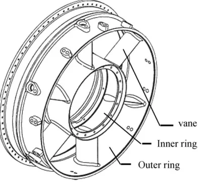
The tail bearing housing (TBH) is a crucial component of most gas turbines and is used to help mount the engine to the body of the aircraft, seeFig. 1. Its major structural details are the outer ring, the inner ring and the vanes. The vanes are usually welded to the rings using the process of Gas Tungsten Arc Welding, frequently known as TIG welding. TIG-welding is a well known welding process applied in the aircraft industry. During welding a high-temperature conducting plasma is created that transfers the thermal energy needed to melt the base material in the work pieces being welded. The arc temperature spans between 12,000 K and 15,000 K above the surface of the weld pool. The mechanical setup during welding is illus-trated inFig. 2. The weld paths used to attach the vanes to the inner ring must be chosen so as to minimize any distortion during the welding process, i.e., the welds can be made in short sub-welds and the ordering

0045-7825/$ - see front matter 2005 Elsevier B.V. All rights reserved. doi:10.1016/j.cma.2005.02.003

*

Corresponding author.

E-mail address:[email protected](I. Voutchkov).

and direction of the individual sub-welds can be interchanged. The selection of such paths is the fundamen-tal structural optimization problem studied in this paper.

Finite element (FE) models, computational fluid dynamics (CFD), statistics, algebraic equations and combinations of these are used to model welding. Which method to use depends on what needs to be ana-lysed[1]. Work on 2D finite element welding simulation began with the first published papers in the early 1970s[2–5] and continues with industrial applications, e.g., welding of small diameter pipes[6]. In 1974, Marcal stated that ‘‘welding is perhaps the most non-linear problem encountered in structural mechanics’’ and this fact has discouraged many from entering the research area[7]. Hibbit and Marcal, then Ph.D. stu-dents, later established one software company each, developing two of the worldÕs most widely used non-linear finite element programs namely ABAQUS and MARC.

The literature also contains a number of works that address the issue of welding sequencing. For exam-ple Kim et al.[8]propose a heuristic method for single-pass welding, which is a modification of the travel-ling salesman method. The authors propose an algorithm for the movement sequence for robot arc welding. Xie and Hsieh[9]propose a modified genetic algorithm (GA) to solve a clamping and welding sequence

Fig. 1. Tail bearing housing.

problem. Teng et al.[10]use a specially designed FE model to assess the stress during a circular weld and to study the effect of the welding sequence. Kadivar et al.[11] utilize a FE model and GA linked with a thermo-mechanical model. Tsai et al. [12] present the optimization of a welding sequence for T-joints, but this is not applicable for the welds discussed in this paper. To the best of our knowledge, no existing work addresses the issue of creating aÔblack-boxÕsurrogate model that can be trained, and later utilized for the prediction or optimization of (welding) sequences, as presented here.

This paper is organised as follows: first the process of FE welding simulation is briefly introduced. Then combinatorial modelling issues are introduced, followed by the surrogate modelling approached proposed here for dealing with combinatorial problems of this kind. Next the surrogate model is applied to the TBH problem and finally, after some discussion, a few brief conclusions are drawn.

2. Surrogate models

In engineering, optimization is often related to improvement of an existing engineering design. Such de-signs can be produced using analytical, computational or experimental data. In many cases this is related to substantial expense in terms of time, resources and money. In order to find a better design, engineers usu-ally try several designs, rejecting the ones that do not meet predefined criteria, while keeping the good ones. This process of trial and selection may involve many expensive design calculations or experiments. That is why, when it comes to optimization, companies tend to opt for small improvements or an existing working design, often abandoning the search for the ultimate optimum design.

The finite element (FE) method in many cases presents the opportunity to replace experimental work with computational assessment, so that optimization work can be carried out using computers rather than real experiments. In cases where FE models exist and are relatively inexpensive to compute, designers can use one of a number of well established optimization methods. However in many areas of engineering FE models have ever increasing complexity and are used mainly for validation of a proposed design. They tend to be accurate and detailed, but very resource demanding. When working with either expensive experiments or expensive computations, it may not be feasible to carry out direct optimization work, as this may greatly increase the cost of the product.

A FE model usually represents many relationships. Not all of them are of interest when improving a design, and therefore it is often possible to create a model that represents only the interesting aspects, which usually are a very small percentage of the total, and thus reduce the expense of simulations. Models that are cheaper representations of a more complex ones are referred to as surrogate models[13]. They represent a few of the many possible relationships, and depending on the modelling approach, they may be more accurate around the area of optimal design than in the rest of the design space. Because surrogate models are so specific about what they model most accurately, they are usually very inexpensive to run. Using such models, many optimi-zation problems that were previously considered unaffordable, have now become possible.

A surrogate model optimization typically includes the following steps:

1. Create a design of experiments detailing initial runs.

2. Evaluate the objective function, experimentally or computationally over these runs with full accuracy. 3. Train a surrogate model that can represent just the desired relationships.

4. Carry out optimization, using the trained surrogate model.

5. Evaluate the optimal design using the expensive method from step 2. 6. Compare the results from the surrogate and the expensive models. 7. If the results agree or are good enough then go to step 9.

The total cost is reduced in step 4, where many function evaluations are needed by the optimization rou-tines. The expensive data used in this work is provided by a validated FE model of a welding process.

3. Welding simulation using finite elements

Welding can cause contractions, which occur when the melted material in the weld pool cools after the arc is removed. This causes stresses of large magnitude to be distributed throughout the component and can also lead to undesirable deformations. These deformations are sensitive to boundary conditions, see for example [14]. In this paper, the finite element (FE) program MSC.MARC 2001r3[15] has been used to undertake the welding simulations. The heat input from the welding process was simulated as a moving heat source where the energy input is distributed as a double ellipsoid; a method first proposed by Goldak [16]. During welding, the stiffness of the component continuously changes as melted material solidifies and the weldment becomes capable of transferring successively greater forces and moments. The effect is that the displacement at the former free edges is successively more constrained. In this sense the welding can be seen as a new boundary condition that is successively activated behind the weld pool.

The new boundary condition is defined as imposing the same displacements and rotations at adjacent nodes on both sides of the weld. Here the joining of material is represented by successively activating two-noded links [15]. The links tie all six mechanical degrees of freedom and the temperature at each end of the link, which lie on opposite sides of the gap in the weld path. These are activated when one of the two nodes reaches the melting temperature[16,17]. There are at least four phenomena that interact with each other and impede the analysis of the final deformations, making the use of non-linear FE essential in making accurate distortion predictions. These are:

(1) The weld sequence determines the order and timing in which the stiffness of the two geometries change due to successively activating new constraints on the former free edges. As in all structural analyses, boundary conditions impact on how the structure responds to loads.

(2) The order in which strains from cooling of the weldment may, depending on the geometry, cause a deformation mode that later cannot be reversed since the structure already has a preferred mode of deformation. The simplest analogy is a two stage loading of a circular bar where the first load F1is perpendicular to the axis and the next loadF2is compression in axial direction. During compres-sion loading the bar deflection will continue in the direction prescribed byF1.

(3) The YoungÕs modulus for the material under study, Inconel 718, falls around 900C. Thus, for tem-peratures ranging from nearly 900C down to room temperature, the solidified weldment imparts stresses to the surrounding material. Cooling of the component is governed by the temperature in the surrounding air relative to the component temperature while the thermal conductivity governs the heat flux that flows from hotter to cooler areas. At the end of a welding sequence it is likely that shrinkage will occur at different rates on various positions around the total welding bath. The stresses from thermal strain can be integrated over the thickness to obtain forces that work in specific direc-tions with different strengths. These forces can be working in the same direction or, as in this study, they can be competing with each other.

These effects can be predicted separately without simulations. However, without FE simulations it is gen-erally not possible to predict accurately the effects in terms of their magnitude and the time at which they appear. Moreover, changing the weld sequences interchanges all these properties in time and/or magnitude. This leads to a combinatorial optimization weld path planning problem.

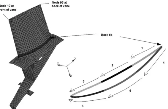
In this paper the welds are broken down into six sub-welds that can be carried out in any order and in either direction, seeFig. 3. The maximum number of sub-welds is defined by the operational characteristics of the robot-arm, which performs the welds. Theoretically, the proposed method should be applicable to any number of sub-welds. The welding on each side of the vane creates a bending moment around an axis in the plane defined by the weld paths. This causes the top of the vane, represented by nodes number 10 and 96, to rotate around that axis, creating displacements at the nodes. In addition there are thermal strains in directions parallel to the weld and in radial direction. The radial thermal strains cannot be eliminated or compensated for in a straightforward way, because no fixturing restrains radial movements at the top of the vanes. Further, the thermal strains parallel to the weld tend to shorten the distance along the weld and create permanent deflections in the plate span of the guiding vane.

Note that the welding analysis performed throughout this paper does not include differential heat input in the thicker sections. The results from the optimization simulations nevertheless showed good correlation to experiments carried out at Volvo Aero with similar geometries. Also the heat transfer from the compo-nent to the surrounding air is governed by assuming a heat transfer coefficient of 12 W/m2K. This might not be the case for an arbitrary geometry. The mechanical boundary conditions used reflect the setup shown inFig. 2.

4. Proposed combinatorial modelling-problem notation and analysis

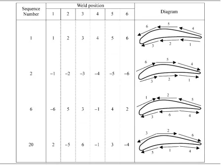
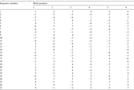
Having discussed welding simulation, and introduced the division of the main weld path into smaller sub-welds, we next introduce the combinatorial modelling aspects of the problem. The notation adopted to describe possible welding sequences is presented inTable 1. Four sequences (labelled 1, 2, 6 and 20) are shown for illustration. In the header row, labels 1–6 designate the six places in a welding sequence. Each

welding sequence contains the names of welding events as illustrated inFig. 3. Theminus sign corresponds to the reverse welding directionto those shown inFig. 3. The dashed line running vertically between columns represents the 5 s gap, used to change and reposition the welding tool. The numbers in the header row cor-respond to the order in the sequence in which the welds have been carried out. Arrows show their directions and positions. The first column is the sequence number of the weld path design, taken from a design of experiments (DoE) approach, which is discussed later in the paper.

As already noted, a finite element model is used to calculate the displacement at various nodes. By way of example, the three components of the displacement at node 10 for welding sequence number 6 are shown

inFig. 4. The curve labelledÔspeedÕshows the speed of the welding tool, and may be used to visualise and

distinguish between the six welding processes and the 5 s cooling gaps. The process completes after 193 s and then the weld is cooled with the clamps on. At second 300, the clamps are released and the cooling continues to room temperature until the end. For the remainder of this study only node 10 is considered, as the figure shows that the other tip node, Node 96, exhibits similar behaviour. The analysis also shows that only the Xcomponent of the displacement needs to be considered for optimization, as it is the most significant and changes in both directions. TheZcomponent is an order of magnitude lower than that inX and therefore does not have significant influence on the resultant displacement. The Y component only

Table 1

changes in the positive direction, and cannot be compensated for by changing the welding sequence. The FE analysis process thus takes as input the welding sequence and produces a displacement diagram for theXcomponent of node 10 over the welding sequence.

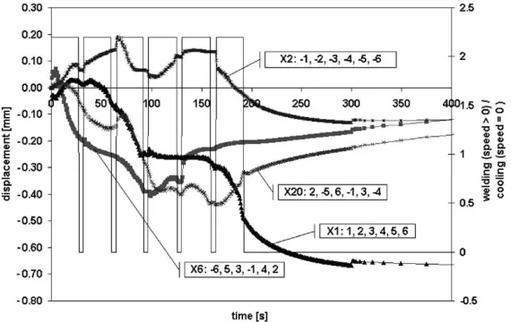
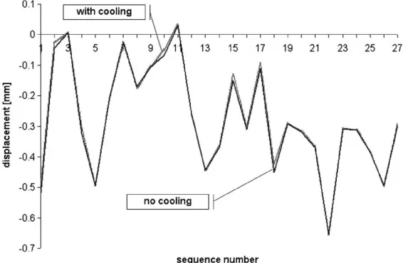
Xdisplacements for runs 1, 2, 6 and 20 fromTable 1 are shown inFig. 5. Note that variation of the welding sequence can significantly change the displacement at node 10, and therefore can be used for opti-mization purposes. In summary, the aim is to reduce theXdisplacement at the time the clamps are released, by changing the welding sequence. We have six variables (one for each welding position), each of which can take 12 non-numerical values (6 for one direction and 6 for the opposite). An obvious solution is to run all possible 46 080 (26·6!) combinations and select the best amongst them. However, this is not feasible when one takes into account that a single welding sequence takes 32 h to analyse using the FE approach.

Fig. 5.Xdisplacements for four welding sequences.

Given this high computational expense, the aim is to optimize the process with a maximum of 50 FE runs. Most of the available combinatorial optimization methods described in the literature would far exceed this number, i.e., integer programming, graph methods, branch and bound, binary trees[18], etc. Therefore, the aim is to reduce the computational expense, by constructing a surrogate model that requires less effort to compute. This model is discussed next.

5. Development of a surrogate for sequential processes

The total permanent displacement caused due to welding can be described as a sum of the displacements caused by the six individual welds and the cooling involved. We propose to represent the overall

displace-mentDby

D¼X

6

i¼1

ðdiþdciÞ þd c

; ð1Þ

as a superposition ofdi, the displacement caused by weld iin the welding sequence,dci the displacement caused by the cooling stage after each weld, and dc the displacement caused by the final cooling stage. To simplify matters, the cooling displacements will be ignored to begin with, so that Eq.(1) becomes

D¼X

6

i¼1

di: ð2Þ

This assumption does not bring a great loss of accuracy, as shown inFig. 6. The agreement shown confirms that the contributions to the overall displacement from the welding process overwhelmingly exceed those from the cooling processes.

Now clearly the displacement caused by a weld will depend on the weld position and direction itself and also any previous welding events. We propose to deal with this dependence by constructing a series model that incrementally captures this process. To begin with, if a weld occurs first in the sequence the displacement

caused is independent of subsequent welds and here we term this amain effect. The main effect for welding eventw, will be denoted asMw. For instance, runs 1, 2, 6 and 20 described earlier give information about

M1,M1,M6andM2respectively. There are six welds each with two possible directions giving a total of 12 possible values of the main effect—these can, of course, be determined by 12 runs of the FE model. More-over, to establish such main effects there is no need to run the whole welding sequence, the first weld from each run will provide complete information on the main effect.

We are now able to consider the simplest possible model, where the final displacement is assumed to be just the sum of the main effects. A model based on this assumption leads to

D¼X

6

i¼1

Mwi; ð3Þ

where,wiis welding eventw, welded atith place in the welding sequence. For example, the displacement for

case 20 inTable 1, using this model would look like

D¼M2þM5þM6þM1þM3þM4:

This surrogate is based on a system without memory. It assumes that the same distortion will arise from a weld wherever it is placed in the sequence (i.e., as though it were the first weld). It does not take into ac-count anything that may have happened internally in the system due to previous welds, such as displace-ment due to internal stresses and thermal deformations. A model based just on Eq. (3) meets our requirement of a low number of FE runs, because it needs only 12 runs to determine each main effect. Unfortunately the system does not behave as a non-memory system, and it turns out that the displacements caused by a given welding event vary significantly with its place in the welding sequence. We next consider a more accurate model

D¼X

6

i¼1

ðMwiþDðw;iÞÞ; ð4Þ

whereD(w,i) is the improvement to the accuracy caused by including the effect of the position of a weld in the sequence.

Let us now introduce some definitions about theorderand thetype of contribution to the overall dis-placement caused by individual welds, here referred to as occurrences. The order of an occurrence will be designated by an appropriate number as a subscript. The type will be designated by primes. To describe the displacement at positioni, we define these as follow:

(i) First order terms of type 1 ignore any contribution of previous weld events, i.e., they represent a sys-tem with no memory. However they do take into account the effect of the position within the sequence. The main effects defined earlier can be considered as first order terms of type 1, but only when they are used to describe the displacement at position 1.

(ii) First order terms of type 2 are the same as above, except that they ignore the effect of sequence posi-tion, for example the model based on Eq. (3) uses just first order terms of types 1 and 2, i.e., in D=M2+M5+M6+M1+M3+M4, M2 is a first order term of type 1, while all of the rest are due to type 2 occurrences, since the contributionsM5,M6,M1,M3andM4, come from

sim-ulations where the welding events5, 6,1, 3 and4, occurred in position 1 of the appropriate weld-ing sequence, but elsewhere in this run.

(iv) Second order terms of type 2, are the same as (iii), however, they again ignore the importance of the position of the pair of events in the overall sequence.

(v) Third order terms, exist only foriP3, and incorporate the two welding events that are immediately before the one under consideration. And so on for higher orders.

Generally, occurrences ofkth order and type 1 will be denoted asR0_kðv;iÞ, wherevis a vector consisting of the welding events at positions [wik+1,. . .,wi1,wi]. Those of type 2 will have a double prime. Consider

k= 1 and type 1: run 20, gives information about the following occurrences of first order:R0₁ð2;1Þ ¼M2;

R0₁ð5;2Þ; R₁0ð6;3Þ; R0₁ð1;4Þ; R0₁ð3;5Þ; R0₁ð4;6Þ. It contains information about the change to the dis-placement caused by the occurrence of various welding events at various positions in the welding sequence. It is not difficult to create a design of experiments (DoE) that will fill the whole first order type one matrix

R0₁ forw=6,. . .,1, 1,. . ., 6; i= 1,. . ., 6. Such a design will have 18 runs.

To describe a system with memory, one needs to account for the effect of present and past occurrences, rather then only present occurrences such asR0₁. Such occurrences are of second and higher order. It is rea-sonable to assume that when considering the last weld in the sequence the effect on its displacement caused by, say, the penultimate weld will be more important than the first. Furthermore, we may postulate that sub-sequences of several welds will have broadly similar effects wherever they occur in the sequence. Using these ideas we can build approximations to the effect of any weld, using the information from runs that have been previously carried out. To do this, we proceed as follows:

1. We predict the deflection after each event, and sum them up. Initially D= 0.

2. Letxpbe the sequence for which we would like to predict the value ofD. For instancexp= [6, 3,5, 4,2, 1].

3. So we start with i= 1 and then increment this at step 12. 4. The highest possible order of occurrence is i.

5. Create vector xp1= [1:i] that contains the first i elements ofxp. For instance for i= 3; xp1= [6, 3,

5].

6. Set k= 1.

7. Create vector xp2=xp1[ik+ 1:i] that takes the lastik+ 1 elements of xp1.

8. Search DoE, forxp2, so that the last element ofxp2, appears atith column of the DoE. If found take the value of the corresponding displacementdiand go to step 10, otherwise continue. The

displace-ment found is an occurrence of orderiand type 1.

9. Search DoE forxp2, anywhere in the DoE. If found take the value of the corresponding displacement diand go to step 10. The displacement found is an occurrence of orderi and type 2.

10. D=D+di.

11. Ifi=wpthen STOP. We have reached the end of the sequence. In the example presented here,wp= 6 which corresponds to 6 welding events per sequence.

12. i=i+ 1 and go to step 4.

To illustrate this process, consider a model based on terms up toR0₂, i.e., up to second order:

D¼Mw1

X6

i¼2

ðMwiþDR

0

1ðv;iÞ þDR20ðv;iÞÞ; ð5Þ

where DR0₁ðv;iÞ ¼DR0₁ðv;iÞ Mwi; DR

0

2ðv;iÞ ¼R02ðv;iÞ Mwi; i is the position in the sequence; v= [wik+1,. . .,wi1,wi], andk= 1 and 2, respectively. Run 20 provides information about the following

R00₂matrix instead. This approximation, which ignores where the sub-sequence pairs have occurred, does not cause a great loss of accuracy. Therefore, the termsR0₂in Eq.(5)can be replaced by

R2ðv;iÞ ¼

R0₂ðv;iÞ if it exists in the DoE;

R00₂ðvÞ if the above does not exists in the DoE;

0 if neither of the above exists in the DoE:

8 > < >

: ð6Þ

To ensure that all occurrences of second order and type 2 exist, 27 FE runs are required. A design of exper-iments using 27 FE runs is discussed later in this paper.

Although such a DoE is designed to include all possible occurrencesR00₂ðvÞ, for some prediction points it will contain occurrences of higher order, which may be used to improve the accuracy further. To do this we then define

HðiÞ ¼

Ri if Ri2DoE; else

Ri1 if Ri12DoE; else ..

.

Mwi if Mwi2DoE; else Mw if Mw 2DoE; else 0 8 > > > > > > > > > < > > > > > > > > > :

ð7Þ

and

D¼X

6

i¼1

HðiÞ ð8Þ

which is a more general form of(5) that finds the sum of the combination of the highest occurrences of lowest type to calculate the predicted value for the displacement for a given welding event and sequence position.

This model can be rewritten for any number of variables, bearing in mind that the highest order of occur-rence is equal to the number of variables. The model exhibits some learning properties, in the sense that it will always produce a prediction if there is at least one point in the DoE and that as the DoE grows in size, the predictions become more accurate. In the limit when all possible combinations have been tested it repro-duces the trial data exactly. This feature allows the model to be used with any number of points in the DoE, giving the freedom to add to the model to achieve any desired accuracy. For the example studied here expe-rience suggests that the existence of the completedR00₂set is enough to ensure a good fit to the existing data. It is obvious that once the trial data has been calculated from a series of FE runs, such a model requires very little computation, and this enables all possible combinations to be examined using the surrogate and the best one selected. This best prediction is then checked using FE, and the results added to the DoE, mak-ing further predictions more accurate. Another full search can then be performed usmak-ing all the points, including the one from the previous run and so on, until successive models produce the same or nearly sim-ilar results.

6. Examples and results

this DoE. The first element of this matrix (1, 1) is equal to 0, since welding event6 cannot be performed after welding event6, (and so all diagonal elements are 0). The element below (2, 1) is equal to one,

show-Table 2

27 point DoE that fills theR00 2matrix

Sequence number Weld position

1 2 3 4 5 6

l 1 2 3 4 5 6

2 1 2 3 4 5 6

3 2 4 6 1 3 5

4 3 5 4 2 6 1

5 4 3 1 6 2 5

6 6 5 3 1 4 2

7 6 1 5 2 4 3

8 6 5 1 4 2 3

9 1 6 4 3 5 2

10 5 4 3 6 2 1

11 4 2 1 6 5 3

12 2 6 4 1 3 5

13 3 6 4 5 1 2

14 5 6 3 2 1 4

15 5 1 3 2 4 6

16 4 1 5 2 6 3

17 3 1 5 2 4 6

18 2 3 5 4 1 6

19 1 2 4 6 5 3

20 2 5 6 1 3 4

21 3 2 6 4 5 1

22 5 3 6 2 1 4

23 6 3 2 5 4 1

24 6 1 5 3 4 2

25 6 2 3 1 5 2

26 3 6 5 2 1 4

27 4 1 2 5 6 3

Table 3 TheR00

2matrix—number of occurrences tested

Present (w)

Weld 6 5 4 3 2 1 1 2 3 4 5 6

Past (w1)

6 0 1 1 1 1 2 1 1 1 1 1 0

5 1 0 1 1 1 1 1 2 1 1 0 1

4 1 1 0 1 1 1 2 1 1 0 1 1

3 1 1 1 0 1 1 1 1 0 1 2 1

2 1 1 2 2 0 1 1 0 1 1 1 1

1 1 1 1 1 2 0 0 1 1 1 1 1

0 3 2 2 2 2 2 2 2 3 2 2 3

1 1 1 1 1 1 0 0 1 1 2 2 1

2 1 1 1 1 0 1 2 0 1 1 1 1

3 1 1 1 0 1 1 1 1 0 1 1 1

4 1 1 0 1 1 1 1 2 1 0 1 1

5 1 0 1 2 1 1 1 2 1 1 0 2

ing that there is one occurrence of the (past, present) pair (5,6). One can find it in run 2, appearing at the 6th position. The row indexed 0 contains the main effects. One can see, for instance, that there are 3 runs giving information for the main effect6. These occur in runs 6, 7 and 23, where welding event6 has been executed first in the welding sequence. This table confirms that there are no zero elements except on the diagonal. The design of experiments, shown in Table 2, was constructed by considering all possible 46 080 combinations in order and selecting the first set that filled all non-diagonal elements in the matrix shown inTable 3.

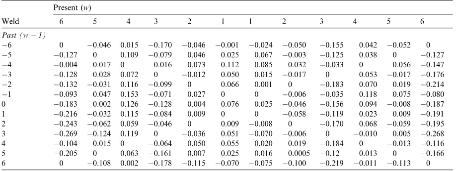
For each element of this matrix, the value of displacement is calculated as the difference of the displace-ment at the end and beginning of a weld, seeTable 4, which has the same structure. So, for instance the displacement caused by the occurrence of the (past, present) pair—(5,6) is0.12721 mm, and this is the value forR00₂ð5;6Þ.

To illustrate the use of this data, consider the following welding sequence:

6 3 -5 4 -2 1

1. D= 0.

2. i= 1: for position number 1, the highest order of occurrence is 1 so, we are checking if there is a main effect for event 6 in the DoE points. Three entries are found (in runs 8, 24, 25): the averaged displace-ment from those runs is used for the first position (actually they are the same). The value is added to D, and now D=M6.

3. i= 2: we proceed with position number 2. The highest order of occurrence is 2, so we check if we can find the pair (6, 3) within the DoE at position 2 (we are first looking for an occurrence of type 1). We cannot find a match, so we continue looking for occurrences of type 2, i.e., a match regardless of posi-tion. One is found in run 27. We add the corresponding value (refinement) to the value ofD, so that

D¼M6þR002ð6;3Þ.

4. i= 3: we proceed with position number 3. The highest order of occurrence is 3, so we check if we can find the set (6, 3,5) within the DoE at position 3 (we are again first looking for an occurrence of type 1). This subset cannot be found in the DoE. The check for this triple, anywhere in the DoE also fails,

Table 4 TheR00

2matrix—displacement values

Present (w)

Weld 6 5 4 3 2 1 1 2 3 4 5 6

Past (w1)

6 0 0.046 0.015 0.170 0.046 0.001 0.024 0.050 0.155 0.042 0.052 0

5 0.127 0 0.109 0.079 0.046 0.025 0.067 0.003 0.125 0.038 0 0.127

4 0.004 0.017 0 0.016 0.073 0.112 0.085 0.032 0.033 0 0.056 0.147

3 0.128 0.028 0.072 0 0.012 0.050 0.015 0.017 0 0.053 0.017 0.176

2 0.132 0.031 0.116 0.099 0 0.066 0.001 0 0.183 0.070 0.019 0.214

1 0.093 0.047 0.153 0.071 0.027 0 0 0.006 0.035 0.118 0.075 0.080

0 0.183 0.002 0.126 0.128 0.004 0.076 0.025 0.046 0.156 0.094 0.008 0.187

1 0.216 0.032 0.115 0.084 0.009 0 0 0.058 0.119 0.023 0.009 0.191

2 0.243 0.062 0.059 0.046 0 0.009 0.008 0 0.170 0.068 0.059 0.195

3 0.269 0.124 0.119 0 0.036 0.051 0.070 0.006 0 0.010 0.005 0.268

4 0.104 0.015 0 0.064 0.050 0.055 0.020 0.019 0.184 0 0.013 0.116

5 0.205 0 0.063 0.161 0.007 0.025 0.016 0.0005 0.12 0.013 0 0.166

indicating that there is no such 3rd order occurrence of either type 1 or 2. Next, we reduce the subset, by truncating the farthest event, which presumably would have the least effect on the deflection, gen-erated at position 3. Now the subset we will be looking for is (3,5). Again we check first for an occurrence of type 1, i.e., such that5 stands at position 3 and event 3 stands at position 2. Such a match is found in run 18. We add it to the value ofD, so thatD¼M6þR002ð6;3Þ þR

0

2ð3;5;3Þ. 5. i= 4: we proceed with position number 4. The highest order of occurrence is 4, so we check if we can

find the set (6, 3,5, 4) within the DoE at position 4 (we are again first looking for an occurrence of type 1). There is no exact match. Now we try for occurrences of type 2, which cannot be found either. We then truncate the subset to (3,5, 4). Again we look for occurrences of type 1 first. There is a match in run 18. We add the appropriate value of refinement contributed by theR0₃term to the value of D, so thatD¼M6þR200ð6;3Þ þR02ð3;5;3Þ þR03ð3;5;4;4Þ.

6. i= 5: we proceed with position number 5. The highest order of occurrence is 5, so we check if we can find the set (6, 3,5, 4,2) within the DoE at position 5 (we are first looking for an occurrence of type 1). Being unable to find an occurrence of 5th order type 1 or type 2, we truncate and look for (3,5, 4,2). The search fails for both type 1 and type 2 occurrences. We then truncate further to (5, 4,2). Again no match is found for either type. Next we try (4,2). There is no occurrence of type 1, but we can find a type 2 occurrence in run 4. We add it to the value of D, so that now

D¼M6þR002ð6;3Þ þR

0

2ð3;5;3Þ þR

0

3ð3;5;4;4Þ þR

00

2ð4;2Þ.

7. i= 6: we proceed with position number 6. The highest order of occurrence is 6, so we check if we can find the set (6, 3,5, 4,2, 1) within the DoE at position 6 and unsurprisingly we cannot find this combination. We go through the same procedure as in the previous stage, checking for occurrences of type 1 and 2, of the following subsets (3,5, 4,2, 1); (5, 4,2, 1); (4,2, 1). None of them is found. Finally, when we look for (2, 1) anywhere in the DoE, regardless of position, we find it in run 14. We add it to the value of D, so that D¼M6þR200ð6;3Þ þR02ð3;5;3Þ þR03ð3;5;4;4Þ þ

R00₂ð4;2Þ þR00₂ð2;1Þ.

The total displacement should also include the final cooling stage, which has been found using a linear curve fit to be reasonably well modelled by

dc¼0:7152Hð6Þ þ0:0143:

Using the above algorithm, the displacement for all possible 46 080 welding sequence combinations may be calculated in less than 5 min on 800 MHz Pentium III machine, using a MATLAB code. A code written in C or FORTRAN would produce results much faster. It has been found that the following sequence, which we labelÔRun 28Õ, produces the least value for jDj

-6 -1 -5 2 -4 3

Run 28

for which the value of the displacement is calculated as follows:

D¼M6þR20ð61;2Þ þR

0

3ð615;3Þ þR

00

2ð5;2;4Þ þR

00

2ð2;4;5Þ þR

00

2ð4;3;6Þ

þ0:7152R00₂ð4;3;6Þ þ0:0143

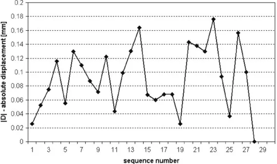
The final optimization result is illustrated inFig. 7, which shows the FE simulation for Run 28 (Dis-placement versus Time). The curve reaches zero dis(Dis-placement just before second 300, when the clamps are released. Run 28 is shown together with some previous runs, for comparison purposes. It illustrates the improvement of theXdisplacement in comparison to Run 1, which is the standard sequence adopted in most TBH production. The values for the displacements for all 28 runs are shown inFig. 8, showing that the optimized run produces minimal displacement.

7. Discussion

The surrogate model introduced in this paper provides a fast and effective method for representing com-putationally expensive FE models that may be used in sequential combinatorial problems. The algorithm

continuously refers to existing information about the system studied by mapping a discrete non-numerical set of information to a continuous numerical domain. To allow it to function with a low number of expen-sive runs, the model predicts following a priority list:

1. Occurrences of highest possible order of type 1. 2. Occurrences of highest possible order of type 2. 3. Occurrences of next highest order of type 1. 4. Occurrences of next highest order of type 2. 5. And so on until.

6. Main effects.

The proposed algorithm will always try to find an item in this list, closest to its beginning. For some problems it might be more suitable to apply the following priority list:

1. Occurrences of highest possible order of type 1. 2. Occurrences of next highest order of type 1. 3. And so on until.

4. Occurrences of highest possible order of type 2. 5. Occurrences of next highest order of type 2. 6. And so on until.

7. Main effects.

Other priority lists are also possible, and could be studied to improve the predictions achieved. Note that the DoE given inTable 2is generated by running six nested loops, each one running through the values6,5,4,3,2,1, 1, 2, 3, 4, 5, 6 and selecting the sequences that obey the following rule:

jAj 6¼ jBj 6¼ jCj 6¼ jDj 6¼ jEj 6¼ jFj;

where A, B,C, D, Eand Fare the six nested loops variables. Each sequence is registered in the matrix, shown in Table 3, and when all but diagonal elements are non-zero, the DoE generation stops. This pro-duces a DoE that contains the first set of sequences that guarantees that allR00

2 occurrences are tested. It should be noted, that this is not necessarily the optimal DoE, nor the smallest possible DoE, although the smallest possible DoE is not expected to be much smaller in size than the one generated.

Clearly, the accuracy of any predictions made depends upon the quantity of information available to the surrogate. In the limit the algorithm will produce a zero deflection for all predictions if no runs are avail-able. For a very rough prediction, one should ensure at least that all the twelve main effects are available, requiring a minimum of at least twelve runs (although these could be truncated to just one sub-weld). For systems that do not exhibit memory, such predictions should be fairly accurate. However, if one desires more accurate predictions, at least second order occurrences of type 2 should be captured, as here.

For higher dimensional problems, one could give greater priority to some positions or events than others. In such cases, a mixed DoE is possible, where the most important events are captured with higher orders of occurrence and the less significant with a lower order. Variations in this respect could lead to re-duced size DoEs, giving most information for the more important events.

8. Conclusions

The method has been applied to the optimization of a welding sequence, and has demonstrated that opti-mum post-weld distortions can be achieved after just 28 FE runs, out of possible 46 080 combinations. This greatly reduces the computational expense needed in weld planning, without significant loss of accuracy. The model has been adapted so that it can be used with any volume of information, allowing for dynamic expansion as more data is made available. This leads to the interesting problem of developing a dynamic optimal design of experiments for sequential combinatorial problems.

Acknowledgements

The authors would like to express their thanks to ITP, Spain for permission to reproduceFig. 1and to the MMFSC project funded by the EU under grant GRD1-1999-10248 for supporting this work.

References

[1] L.E. Lindgren, Modelling for residual stresses and deformations due to welding and ‘‘Knowing what isnÕt necessary to do’’, Keynote of the 6th Int. Seminar in Numerical Analysis of Weldability, Austria, Graz, 2001.

[2] Y. Fujita, Y. Takeshi, M. Kitamura, T. Nomoto, Welding stresses with special reference to cracking, iiw Doc X-665-72, 1972. [3] Y. Ueda, T. Yamakawa, Analysis of thermal elastic–plastic stress and strain during welding by finite element method, Trans.

JWRI 2 (1971) 90–100.

[4] Y. Ueda, T. Yamakawa, Thermal stress analysis of metals with temperature dependent mechanical properties, in: Proc. of Int. Conf. on Mechanical Behaviour of Materials, vol. 3, 1971, pp. 10–20.

[5] Hibbit, Marcal, A numerical thermo-mechanical model for the welding and subsequent loading of a fabricated structure, Comput. Struct. 3 (1973) 1145–1174.

[6] U. Chandra, Determination of stresses due to girth-butt welds in pipes, ASME J. Pressure Vessel Technol. 107 (May) (1985). [7] J. Goldak, B. Patel, M. Bibby, J. Moore, Computational weld mechanics, AGARD Workshop, Structures and Materials 61st

Panel Meeting, 1985.

[8] K. Kim, B. Norman, B. Nnaji, Heuristics for single-pass welding task sequencing, Int. J. Production Res. 40 (12) (2002) 2769– 2788.

[9] L. Xie, C. Hsieh, Clamping and welding sequence optimization for minimizing cycle time and assembly deformation, Int. J. Mater. Product Technol. 17 (5/6) (2002) 389–400.

[10] T. Teng, P. Chang, W. Tseng, Effect of welding sequences on residual stresses, Comput. Struct. 81 (2003) 273–286.

[11] M. Kadivar, K. Jafarpur, G. Baradaran, Optimizing welding sequence with genetic algorithm, Comput. Mech. 26 (2000) 514–519. [12] C. Tsai, S. Park, W. Cheng, Welding distortion of a thin-plate panel structure, American Welding Society—Welding Research

Supplement. Available from:<http://www.aws.org/wj/supplement/supplement2.html>.

[13] D. Jones, M. Schonlau, W. Welch, Efficient global optimization of expensive black box functions, J. Global Optim. 13 (1998) 455– 492.

[14] S. Timoshenko, in: Theory of Elasticity Engineering Societies Monograph, McGraw-Hill Book Company, 1934. [15] MSC.MARC Palo Alto, 2001.

[16] J.A. Goldak, A. Chacravarti, M.J. Bibby, A new finite element model for welding heat sources, AIME 15B (2) (1984). [17] Na¨slund, Jo¨rgen, Welding simulation using the finite element method, joining of geometries, Master thesis, Lulea Technical

University, ISSN 1402-1617/ISRN LTU-EX–00/330–SE/NR 2000:330, 2000 (in Swedish).